On temperature-dependent anisotropies of upper critical field and London penetration depth
V. G. Kogan, R. Prozorov, A. E. Koshelev
TL;DR
This paper demonstrates that in certain single-band superconductors with anisotropic Fermi surfaces, the anisotropies of the upper critical field and London penetration depth vary with temperature, challenging the common multi-band interpretation.
Contribution
It provides a detailed analysis of temperature-dependent anisotropies in single-band superconductors, highlighting factors influencing their behavior and conditions for their temperature dependence directions.
Findings
Anisotropies $\gamma_H$ and $\gamma_\lambda$ depend on temperature in single-band materials.
The temperature dependence can be opposite or same for the two anisotropies.
Fermi surface shape and gap nodes influence anisotropy behavior.
Abstract
We show on a few examples of one-band materials with spheroidal Fermi surfaces and anisotropic order parameters that anisotropies of the upper critical field and of the London penetration depth depend on temperature, the feature commonly attributed to multi-band superconductors. The parameters and may have opposite temperature dependencies or may change in the same direction depending on Fermi surface shape and on character of the gap nodes. For two-band systems, the behavior of anisotropies is affected by the ratios of bands densities of states, Fermi velocities, anisotropies, and order parameters. We investigate in detail the conditions determining the directions of temperature dependences of the two anisotropy factors.
Click any figure to enlarge with its caption.
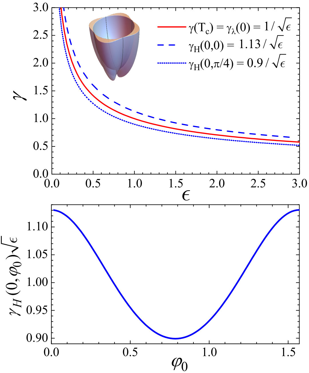 Figure 1
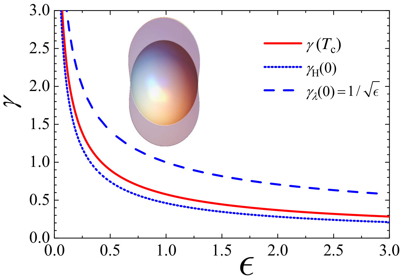 Figure 2
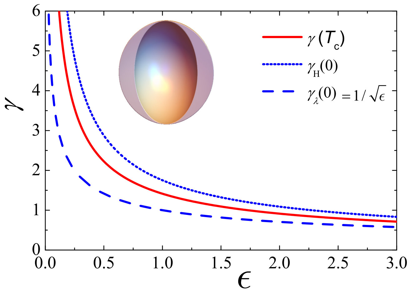 Figure 3
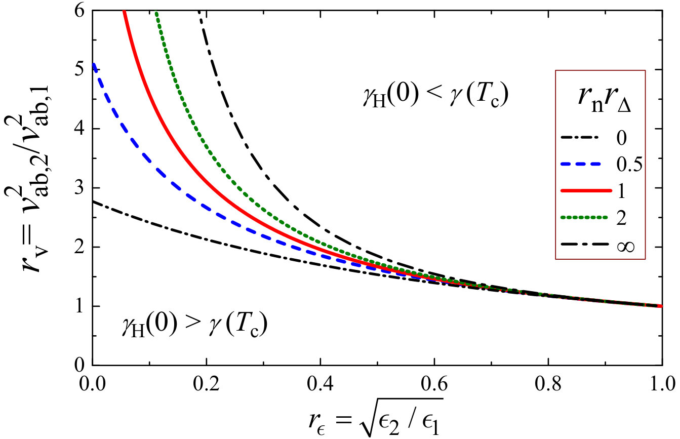 Figure 4
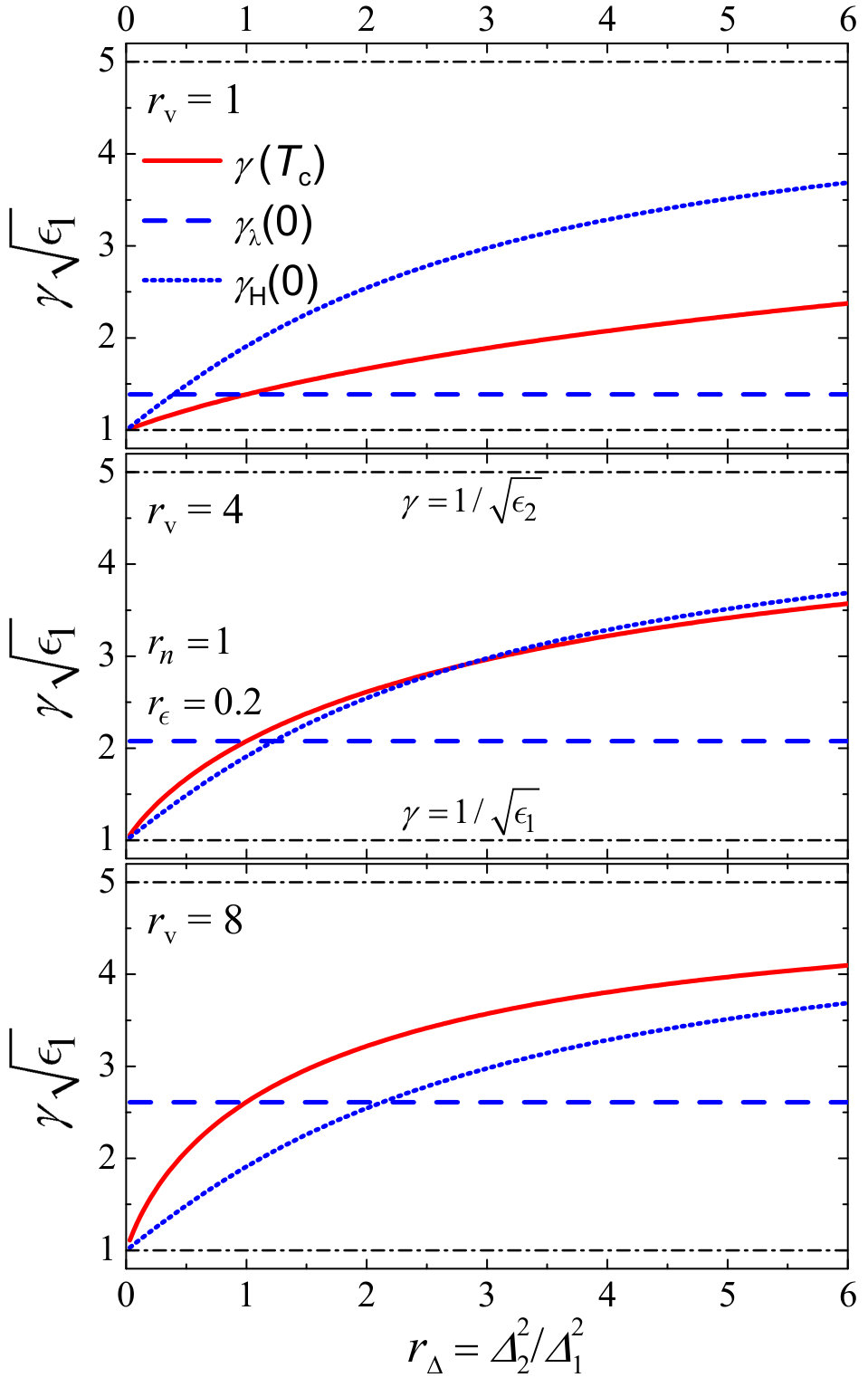 Figure 5
Peer Reviews
No public reviews on file for this paper yet. If you reviewed it on a platform where reviews are public (OpenReview, ICLR, NeurIPS, ICML), you can paste yours below so the community can read it here.
Videos
No videos yet. Explain this paper in a talk, walkthrough, or lecture? Add one.
On temperature-dependent anisotropies of
upper critical field and London penetration depth
V. G. Kogan
The Ames Laboratory and Department of Physics and Astronomy Iowa State University, Ames, IA 50011
R. Prozorov
The Ames Laboratory and Department of Physics and Astronomy Iowa State University, Ames, IA 50011
A. E. Koshelev
Materials Science Division, Argonne National Laboratory, 9700 South Cass Ave., Lemont, Illinois, 60439
(3 July 2019 )
Abstract
We show on a few examples of one-band materials with spheroidal Fermi surfaces and anisotropic order parameters that anisotropies of the upper critical field and of the London penetration depth depend on temperature, the feature commonly attributed to multi-band superconductors. The parameters and may have opposite temperature dependencies or may change in the same direction depending on Fermi surface shape and on character of the gap nodes. For two-band systems, the behavior of anisotropies is affected by the ratios of bands densities of states, Fermi velocities, anisotropies, and order parameters. We investigate in detail the conditions determining the directions of temperature dependences of the two anisotropy factors.
I Introduction
In many superconductors anisotropy parameters of the upper critical field, , and of the London penetration depth, , are not equal. Moreover, they may have different temperature dependencies. In conventional one-band s-wave materials, these parameters for a long time were considered the same and independent. MgB2 is a good example of the current situation: decreases on warming, whereas increases Budko ; AngstPRL02 ; LyardPRB02 ; RydhPRB04 ; Carrington . Up to date, the dependence of the anisotropy parameters is considered by many as caused by a multi-band character of materials in question with the common reference to MgB2. In this work we develop an approximate method to evaluate that can be applied with minor modifications to various situations of different order parameter symmetries and Fermi surfaces, two bands included. In particular, we show that even in the one-band case ’s and their dependencies may differ if the Fermi surface is not a sphere or the order parameter is not pure s-wave. Our conclusions challenge the common belief that temperature dependence of is always related to multi-band topology of Fermi surfaces.
We focus on the clean limit for two major reasons. Commonly after discovery of a new superconductor, an effort is made to obtain as clean single crystals as possible since those provide a better chance to study the underlying physics. A proper description of scattering in multi-band case would have lead to a multitude of scattering parameters which cannot be easily controlled or separately measured. Besides, in general, the scattering suppresses the anisotropy of , the central quantity of interest in this work.
To begin, it is worth recalling that the problem of the second-order phase transition at the upper critical field has little in common with the problem of a weak field penetration into superconductors, thus a priori one should not expect . Still, at the critical temperature the Ginzburg-Landau (GL) theory requires because both are described in terms of the same mass tensor.
At , the order parameter , and Eilenberger equations for weak coupling superconductors can be linearized. The factor here describes the dependence of and is normalized so that the average over the full Fermi surface .
At the second-order phase transition at , the basic self-consistency equation of the theory can be written as ROPP :
[TABLE]
Here, is the Fermi velocity, , is the vector potential, and is the flux quantum. In comparison to the traditional form of this equation involving sums over the Matsubara frequencies, this form contains only integrals relatively easy to deal with.
Typically, the temperature dependences of the anisotropy factors are monotonic. Therefore, to determine the direction of these dependences, it is sufficient to evaluate anisotropy values at the transition temperature and at .
I.1 and at
In this domain, the gradients ( is the order of magnitude of the coherence length), and one can keep in the expansion of in the integrand (1) only the linear term to obtain:
[TABLE]
This is, in fact, the anisotropic version of linearized GL equation with Gorkov
[TABLE]
The anisotropy parameter for uniaxial materials then readily follows:
[TABLE]
As mentioned above, the anisotropy of the London penetration depth at is the same as that of :
[TABLE]
This can be proven also directly using a general expression for the tensor , see e.g. gam-lam0 . Since always coincides with , in further considerations we drop the subscript, i.e., .
In the following we adopt Fermi surface as a spheroid with the symmetry axis . The Fermi surface average of a function is evaluated in the Appendix A:
[TABLE]
Hear is the squared ratio of spheroid axes, and are the polar and azimuthal angles, respectively.
I.2 and at
The low-temperature orbital determined by Eq. (1) can be approximately evaluated using variational approach with the anisotropic lowest Landau level wave function as a trial, see Appendix B. This gives the low-temperature anisotropy factor
[TABLE]
where the optimal variational parameter has to be evaluated from equation
[TABLE]
According to Ref. gam-lam0 , the anisotropy of the penetration depth at in the clean case is given by
[TABLE]
Neither gap nor its anisotropy enter this result, i.e. in the clean case depends only on the shape of the Fermi surface. The physical reason for this is the Galilean invariance of the superflow in the absence of scattering: looking at the superflow in the frame attached to a moving element, one sees all charged particles taking part in the supercurrent independently of their energy spectrum, so that the penetration depth depends only on the total carriers density.
II Single-band anisotropies
II.1 , isotropic s-wave.
We start with the simplest case of a constant gap on a Fermi spheroid. In this case both at and . With the help of Appendix A, we find
[TABLE]
Thus, and it is independent. In particular, this means that as well. In fact, this is just GL results: at , .
To find we note that the trial lowest Landau wave function with is actually exact solution of Eq. (1) for the in-plane field orientation. In this case Eq. (7) in spherical coordinates takes the form:
[TABLE]
One can show that the double integral here vanishes meaning that . Thus, for isotropic s-wave, temperature independent anisotropies are .
II.2 , d-wave on Fermi spheroid
If the spheroid symmetry axis coincides with of the d order parameter, the standard normalization gives . Since zero- anisotropy of is independent of the order parameter symmetry, we have , the same as for s-wave. This is the case of all examples considered in this section. At we have:
[TABLE]
and, according to Eq. (5), . Hence, -anisotropies for s- and d-wave symmetries are the same, that is somewhat surprising.
The calculation of the low-temperature anisotropy from Eqs. (7) and (8) is more involved. In addition, with decreasing temperature the in-plane upper critical field acquires dependence on the azimuth angle between the field and direction of the maximal order parameter. Correspondingly, the anisotropy factor also has such dependence. We will keep the axis along the direction of magnetic field, meaning that the weight function in the angular averaging has to be modified as . The angular averages in Eqs. (7) and (8) can be done analytically. The results, however, are somewhat cumbersome and presented in the Appendix B.1.1. The computed dependences of on the ellipticity are shown in the upper panel of Fig. 1. The blue dashed curve is , the dotted-blue is , and the red solid curve is . Hence, decreases on warming by 13%, whereas increases by 10%. We also note that the anisotropy at is temperature independent. At the lower panel we show the angular dependence of the product which does not depend of . Hence, one expects the in-plane to vary by about 25% being rotated relative to the crystal axis leading to the same variation of the .
II.3 , an equatorial line node
The equatorial nodal line is a feature for one of realizations of the p-wave order parameter. Again, at one has . The anisotropy factor at is
[TABLE]
where and . Integrations here can be done analytically and the result is presented in Appendix B.1.2. The computed anisotropy factor at is plotted as the solid-red curve in Fig. 2. We can see that the shape of order parameter reduces this factor in comparison with the Fermi-surface anisotropy which is represented by (blue dashed line). As a consequence, decreases substantially on warming.
For evaluating , we need to compute averages in Eqs. (7) and (8). The normalization constant from the condition can be found as
[TABLE]
(for ), see Appendix B.1.2. The average in Eq. (8) for the optimal variational anisotropy factor can be reduced to
[TABLE]
This integral can be taken analytically leading to a somewhat cumbersome result which is presented in Appendix B.1.2. The angular average in Eq. (7) for the zero-temperature anisotropy can be reduced to the following integral
[TABLE]
which we compute numerically. The resulting dependence of vs is shown by the blue-dotted curve in Fig. 2. We can see that it is smaller than meaning that it is reduced even stronger with respect to the Fermi surface anisotropy . Thus, decreases on warming whereas is slightly increasing.
II.4 , two polar point nodes
Two polar point nodes also may realize in the case of the p-wave order parameter. Calculations in this case are similar to the previous one. Similar to Eq. (13), the anisotropy factor at is
[TABLE]
The analytical result is given in Appendix B.1.3. The computed anisotropy factor at is presented in Fig. 3 by the solid-red curve. We can see that, in contrast to the case of equatorial node line, the order-parameter anisotropy enlarges this factor in comparison with the Fermi-surface anisotropy (blue dashed line). Consequently, increases on warming.
To compute , we again have to evaluate averages in Eqs. (7) and (8). The normalization constant has to be found from the condition . As , we can use the result from Appendix B.1.3 giving in the case
[TABLE]
The average in Eq. (8) for the optimal variational anisotropy factor now becomes
[TABLE]
We present the analytic result for this integral in Appendix B.1.3. The angular average in Eq. (7) for the can be reduced to the integral
[TABLE]
which we compute numerically. The calculated dependence of vs is shown in Fig. 3 by the blue-dotted curve. We can see that it is larger than meaning that it is enlarged even stronger with respect to the Fermi-surface anisotropy . Thus, increases and decreases on warming, opposite to the case of an equatorial node line.
III Two s-wave bands
Many materials have multiple nonequivalent bands with different superconducting gaps. The most notable examples are magnesium diboride and iron-based superconductors. The two-band model is the simplest model addressing this situation allowing for qualitative understanding of multiple-band effects. The iron-based superconductors may have symmetry meaning that the order parameter has opposite signs in different bands. The relative sign of order parameter, however, is irrelevant for the behavior of anisotropies in clean materials.
We consider two spheroidal Fermi surfaces with constant s-wave gaps. Therefore, each band is characterized by four parameters: the in-plane effective masses , anisotropies , band depths (distances between the Fermi level and the band’s bottom or top), and gaps . Here and below is the band’s index. Note that whether the band has an electron or hole character does not play any role in our consideration and notates here the absolute value of the effective mass. Relative properties of the bands may be characterized by four ratio , , , and .
This two-band model corresponds to the gap anisotropy given by
[TABLE]
where are two sheets of the Fermi surface and are constants. We denote the densities of states (DOS) on the two parts as ,
[TABLE]
Assuming being constant at each sheet, we have:
[TABLE]
where , are normalized DOS’ with and their ratio is related to the above parameters as . Since the average over the full Fermi surface , one has
[TABLE]
meaning that . The ratio of the ’superconducting band weights’ is .
Within this model we obtain:
[TABLE]
The ratios of average squared velocities are obtained using Appendix A and Eqs. (10):
[TABLE]
The results for the anisotropy factors look simpler when expressed via ratios and instead of and . We can express and in terms of the introduced ratios as
[TABLE]
The variational estimate for the low-temperature anisotropy is described in Appendix B.2 and leads to the following result
[TABLE]
with ,
[TABLE]
and . Comparing these equation with Eq. (27), we see that the ratio is determined by only three parameters, , , and the product corresponding to the ratio of the condensation energies, .
Equations (27), (28), (29), and (30) give general results for the anisotropy factors of two-band s-wave superconductors in terms of the band-parameter ratios. As the band numbering is arbitrary, all anisotropies are invariant with respect to the substitutions and for all ratios. For definiteness, we will assume that the second band has higher anisotropy, i.e., . We observe that, as expected, in the case of identical ellipticities all anisotropies are temperature independent and equal to independently of other ratios. As function of the DOS’ ratio , all three anisotropy factors interpolate in between for and for . At intermediate , however, we can observe that the bands contribute to different anisotropies with different weights, and one may have many situations.
The simplicity of this model notwithstanding, when applied, e.g., to the problem of -dependence of anisotropies in MgB2 gam-lam0 , it reproduces well the observed behavior. The unique feature of MgB2 is that and have opposite temperature dependences: increases with warming from \sim$$1 to \sim$$2, while drops from \sim$$5-6 to \sim$$2 AngstPRL02 ; LyardPRB02 ; RydhPRB04 ; Carrington . This behavior is consistent with multiband superconducting properties of this material. It has two groups of bands, three-dimensional -bands with smaller gap and quasi-two-dimensional -bands with larger gap. The band parameters are gam-lam0 (-band), (-band), , , and . Then Eqs. (27), (28), and (29) give , , and , which is roughly consistent with experiment.
The most interesting question is what band properties determine the direction of temperature dependences of the anisotropy factors. In the case of this question has a straightforward and simple answer. From Eqs. (27) and (28), we derive a relation
[TABLE]
which shows that the direction of the temperature dependence is determined only by relations between the bands anisotropies and gaps. In particular, increases on warming if the band with higher anisotropy has also larger gap (like in MgB2), and decreases otherwise.
The case of is more involved. The simple criterion can be obtained only in the case of small difference between the ellipticities . In this case expansion with respect to small parameter gives
[TABLE]
indicating that increases on warming if the band with higher anisotropy has larger Fermi velocity. When the band anisotropies are not close, there is no simple criterion determining the direction of the temperature dependence. In the case , decreases with temperature at very small Fermi-velocity ratios and vice versa. The value of separating the two regimes depends on two parameters, and . Analytical results for this quantity can be derived in the limiting cases and .
[TABLE]
Figure 4 shows these limiting velocity ratios together with the numerically computed dependences for three intermediate values of the condensation-energy ratio , , , and . We can see that the separating increases with decreasing and also grows with increasing . The sensitivity to the latter parameter increases with decreasing . In particular, MgB2 is located in the lower left corner of this plot.
To illustrate typical behaviors of the anisotropy factors, we present in Fig. 5 their dependences on the ratio characterizing a relative strength of superconductivity in two bands. The plots are made for , and three values of the Fermi velocity ratio , , , and . In the first case is below in Eq. (33) meaning that exceeds in the whole range of and always decreases on warming. In the range such situation qualitatively corresponds to magnesium diboride. The last value exceeds given by Eq. (34) and the behavior is opposite, always increases with temperature. The intermediate value is in between and . In this case the behavior of switches with increasing : is smaller than for small and exceeds for . While does not depend on , both and increase with interpolating between for and for . Consequently, the latter two anisotropies always cross . In particular, as mentioned above, decreases on warming at and increases with temperature at . Therefore, depending on the band parameters, all possible six relations between the three anisotropy factors may be realized.
IV Summary
It is shown that the anisotropy parameters, for the upper critical field and for the penetration depth, in general, depend on temperature even in one-band materials with anisotropic order parameters. The temperature behavior of ’s depends, in particular, on the order parameter nodes and their distributions.
We provide four examples of gap anisotropies. In the simplest reference case of isotropic s-wave, and is independent. For d-wave symmetry with coinciding polar axis of the order parameter and of Fermi spheroid, is the same as for s-wave and is independent. is weakly changing on warming, with the sign of this change depending on what direction of in-plane field is chosen for determination of the anisotropy parameter, see Fig. 1. If has a line node on the equator of Fermi spheroid, decreases on warming whereas increases, see Fig. 2. Point nodes at spheroid poles affect anisotropies in opposite way as demonstrated in Fig. 3. In general, the former/latter behavior is realized in the cases when the gap at the equator is smaller/larger than the gap at the poles.
In the case of two spheroidal Fermi surfaces, we investigated in detail the conditions determining directions of temperature dependences of the anisotropy factors. We found that increases with temperature only if the band with higher anisotropy has larger gap independently on relations between other band parameters. The behavior of is more complicated. In general, increases with temperature if the Fermi velocity of the more anisotropic band sufficiently exceeds the Fermi velocity of the less anisotropic band. The Fermi-velocity ratio separating the two regimes depends in a nontrivial way on the ratios of band anisotropies and condensation energies, as illustrated in Fig. 4. In general, all six possible relations between three key anisotropy factors, , , and , may be realized for different relations between band parameters, see Fig. 5.
Our results for Fermi ellipsoids are based on theory ROPP , which is a generalization of Helfand-Werthamer work HW for the isotropic case. One of the features of this approach is that solutions of the linear equation at , belonging to the lowest Landau level, satisfy also the self-consistency equation for superconductivity. For general Fermi surfaces this is not the case and the exact solution can be obtained using expansion over full set of the Landau-level wave functions, see e.g. Refs. RieckPhysB90 ; Kita . In this paper, we employ a much simpler approximate variational approach using the lowest-Landau wave function as a trial. This approach leads to reasonable results suitable for qualitative interpretations of data on anisotropy parameters.
Also, it is worth keeping in mind that we estimate the anisotropy of orbital and disregard possibility of Pauli limiting effects. The decreasing anisotropy with decreasing temperature, like, e.g., in iron pnictides Yuan2009 ; Khim2011 ; Meier2016 , is usually considered as an indication of strong paramagnetic effect. While this interpretation in many cases is correct, we point out that such a behavior may also be realized in purely orbital case, as illustrated in Figs. 2 and 5. Even though modeling many-band systems with two Fermi ellipsoids is far from being realistic, this simple approach still provides some straightforward inroads to a complicated interplay of anisotropies and .
Acknowledgements.
This work was supported by the U.S. Department of Energy (DOE), Office of Science, Basic Energy Sciences, Materials Science and Engineering Division. The research of VK and RP was performed at Ames Laboratory, which is operated for the U.S. DOE by Iowa State University under contract # DE-AC02-07CH11358. The work of AK in Argonne was supported by the U.S. Department of Energy, Office of Science, Basic Energy Sciences, Materials Sciences and Engineering Division.
Appendix A Fermi spheroid
The Fermi surface as an ellipsoid of rotation is an interesting example in its own right and as a model for calculating and in uniaxial materials. Since both of these quantities are derived employing integrals over the full Fermi surface, they are weakly sensitive to fine details of Fermi surfaces.
Although straightforward, the averaging over the Fermi spheroid of the main text should be done with care. Moreover, there are examples in literature where these averages were done incorrectly MMK ; ROPP . We reproduce here this procedure to correct the error and to prevent it in future.
Consider an uniaxial superconductor with the electronic spectrum
[TABLE]
so that the Fermi surface is an ellipsoid of rotation with as the symmetry axis. In spherical coordinates
[TABLE]
so that
[TABLE]
The Fermi velocity is , with the derivatives taken at :
[TABLE]
The value of the Fermi velocity, , is
[TABLE]
The density of states is defined as an integral over the Fermi surface:
[TABLE]
An area element of the spheroid surface is
[TABLE]
and after simple algebra one obtains:
[TABLE]
where . This gives
[TABLE]
The normalized local density of states within solid angle is
[TABLE]
Eq. (43) has been used here. Thus, the Fermi surface average of a function is:
[TABLE]
Appendix B Variational estimate of the upper critical field
Equation for the upper critical field (1) has exact solution only in few special cases. In general situation the exact numerical solution may be obtained, for example, by expansion over a complete set of Landau-level wave functions RieckPhysB90 ; MMK . An approximate solution giving in many cases a reasonable accuracy may be obtained using the variational approach DahmPRL03 . The equation (1) corresponds to the following variational problem
[TABLE]
where the maximum has to be found over all possible trial functions . Consider, for definiteness, the magnetic field along the axis. The simplest and most natural choice for the trial function is the lowest Landau-level solution of anisotropic equation for particle with charge in magnetic field
[TABLE]
with , , where the anisotropy factor is the variational parameter. We will assume that is normalized, .
The integral in Eq. (47) is determined by the matrix element , where we use notation . To evaluate this matrix element, we introduce the operators and represent the product as
[TABLE]
where . Note that . Using the relations , , and , we transform
[TABLE]
This relation allows us to evaluate the matrix element as
[TABLE]
leading to the variational equation for the upper critical field,
[TABLE]
In the zero-temperature limit this equation becomes
[TABLE]
As with , we obtain
[TABLE]
Introducing typical velocity scale , we finally arrive at
[TABLE]
The optimal anisotropy factor is determined by equation
[TABLE]
giving
[TABLE]
It is straightforward to demonstrate that in the case of single spheroidal Fermi surface and isotropic order parameter, and Eq. (51) gives the exact -axis upper critical field.
In this paper we only consider crystals isotropic within the plane. In this case the optimal anisotropy factor for field along the axis is obviously equal to one and
[TABLE]
From Eqs. (51) and (53), we obtain the variational estimate for the low-temperature anisotropy factor
[TABLE]
where has to be evaluated from Eq. (52).
B.1 Singe-band cases
B.1.1 D-wave order parameter
In this subsection we summarize the calculations for the case of d-wave order parameter for which the weight function has the form with being the angle between the in-plane component of the magnetic field and the direction of maximum order parameter. In this case evaluation of the integral in Eq. (8) gives
[TABLE]
with . We find that numerical solution of Eq. (8) is very close to the simple dependence . Note that the result is exact.
The average in Eq. (7) can be evaluated as
[TABLE]
giving
[TABLE]
This equation together with above dependence determine the low-temperature anisotropy of , which depends on the azimuth angle . In particular, , , and .
B.1.2 Equatorial line node
Here we summarize the calculations for the case of the order parameter with an equatorial nodal line for which the weight function has the form . For the anisotropy at the integration in Eq. (13) gives
[TABLE]
for . This dependence is plotted in Fig. 2 by a red line.
The calculation of requires the normalization constant . The normalization condition using
[TABLE]
gives Eq. (14).
The integration in Eq. (15) can be performed analytically giving
[TABLE]
The optimal anisotropy factor corresponding to the vanishing of the right hand side can be evaluated numerically.
B.1.3 Two polar point nodes
Here we summarize the calculations for the case of the order parameter with two polar point nodes for which the weight function has the form . For the anisotropy at the integration in Eq. (13) gives
[TABLE]
for . This dependence is plotted in Fig. 3 by a red line.
The integral in Eq. (19) can be taken analytically. In the case the result is
[TABLE]
B.2 Two spheroidal Fermi surfaces
For the case of two spheroids, Eq. (8) for the optimal anisotropy factor becomes
[TABLE]
with the band weights . The averages in this equation can be evaluated as
[TABLE]
This gives the equation for
[TABLE]
which has the following solution
[TABLE]
with .
The low-temperature anisotropy factor is connected with by Eq. (7). Computing the averages
[TABLE]
we finally obtain
[TABLE]
This equation together with Eq. (57) gives the approximate variational estimate for the low-temperature anisotropy of the upper critical field in the case of two spheroidal Fermi surfaces with isotropic s-wave order parameters.
The reference list from the paper itself. Each links out to its DOI / PubMed record.
- 1(1) S.L. Bud’ko, P.C. Canfield, V.G. Kogan, Physica C Superconductivity, 382 , 85 (2002).
- 2(2) M. Angst, R. Puzniak, A. Wisniewski, J. Jun, S. M. Kazakov, J. Karpinski, J. Roos, and H. Keller Phys. Rev. Lett. 88 , 167004 (2002).
- 3(3) L. Lyard, P. Samuely, P. Szabo, T. Klein, C. Marcenat, L. Paulius, K. H. P. Kim, C. U. Jung, H.-S. Lee, B. Kang, S. Choi, S.-I. Lee, J. Marcus, S. Blanchard, A. G. M. Jansen, U. Welp, G. Karapetrov, and W. K. Kwok Phys. Rev. B 66 , 180502(R) (2002).
- 4(4) A. Rydh, U. Welp, A. E. Koshelev, W. K. Kwok, G. W. Crabtree, R. Brusetti, L. Lyard, T. Klein, C. Marcenat, B. Kang, K. H. Kim, K. H. P. Kim, H.-S. Lee, and S.-I. Lee, Phys. Rev. B 70 , 132503 (2004).
- 5(5) J.D. Fletcher, A. Carrington, O.J. Taylor, S.M. Kazakov, J. Karpinski, Phys. Rev. Lett. 95 , 097005 (2005).
- 6(6) V.G. Kogan and R. Prozorov, Reports on Progress in Physics 75 , 114502 (2012).
- 7(7) L.P. Gor’kov and T.K. Melik-Barkhudarov, Zh. Eksp. Teor. Fiz. 45 , 1493 (1963) [Sov. Phys. JETP 18 , 1031 (1964));
- 8(8) V.G. Kogan, Phys. Rev. B 66 , 020509 (2002).