Defect-like structures and localized patterns in SH357
Edgar Knobloch, Hannes Uecker, Daniel Wetzel

TL;DR
This paper investigates the complex pattern formation in the SH357 equation, revealing bistability, localized structures, and diverse steady states through numerical analysis and bifurcation studies.
Contribution
It provides a detailed numerical study of the SH357 equation, uncovering new localized defect-like structures and complex bifurcation phenomena.
Findings
Bistability between small and large amplitude stripes.
Existence of heteroclinic connections and localized defect-like structures.
Rich variety of stable steady states with different stripe configurations.
Abstract
We study numerically the cubic-quintic-septic Swift-Hohenberg (SH357) equation on bounded one-dimensional domains. Under appropriate conditions stripes with wave number bifurcate supercritically from the zero state and form S-shaped branches resulting in bistability between small and large amplitude stripes. Within this bistability range we find stationary heteroclinic connections or fronts between small and large amplitude stripes, and demonstrate that the associated spatially localized defect-like structures either snake or fall on isolas. In other parameter regimes we also find heteroclinic connections to spatially homogeneous states, and a multitude of dynamically stable steady states consisting of patches of small and large amplitude stripes with different wave numbers or of spatially homogeneous patches. The SH357 equation is thus extremely rich in the types of…
Click any figure to enlarge with its caption.
 Figure 1
 Figure 2
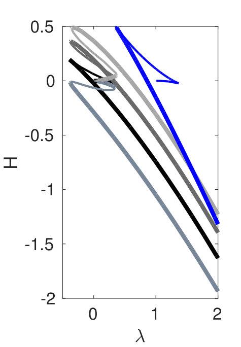 Figure 3
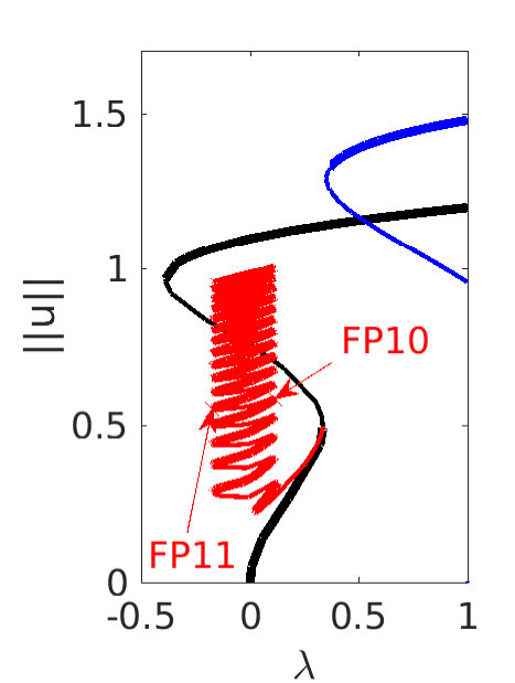 Figure 4
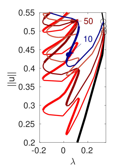 Figure 5
 Figure 6
 Figure 7
 Figure 8
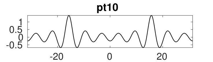 Figure 9
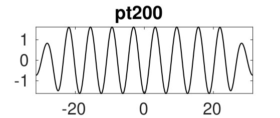 Figure 10
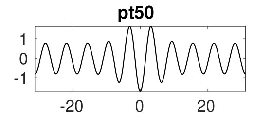 Figure 11
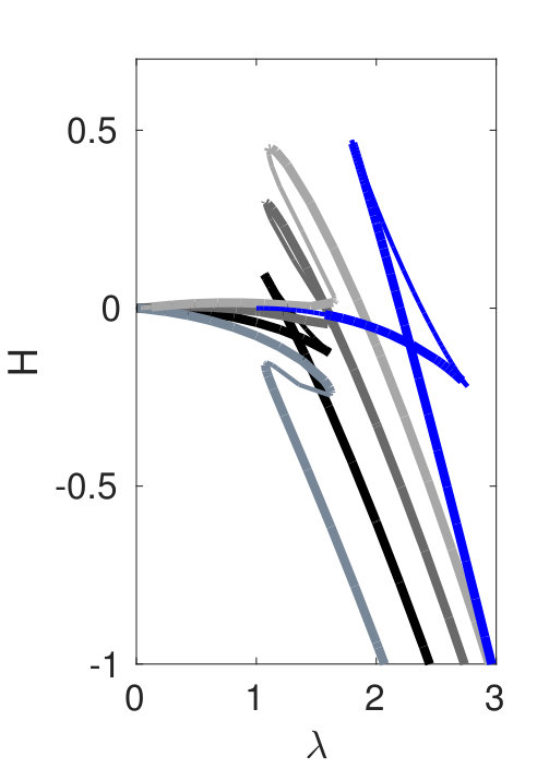 Figure 12
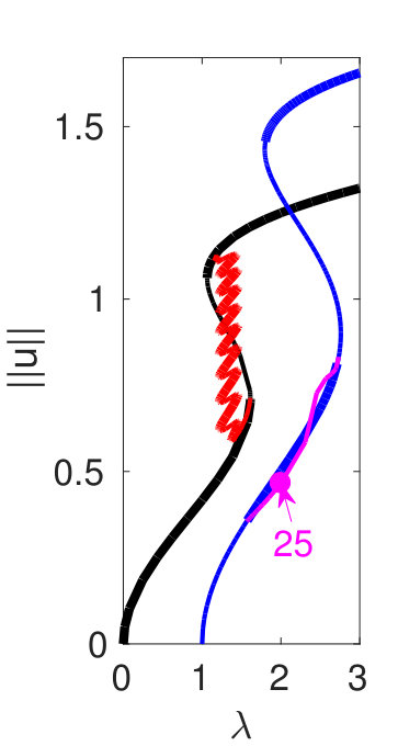 Figure 13
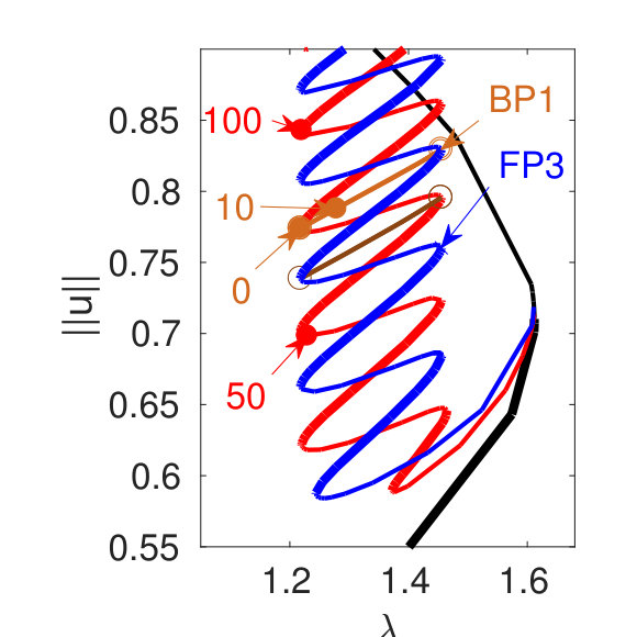 Figure 14
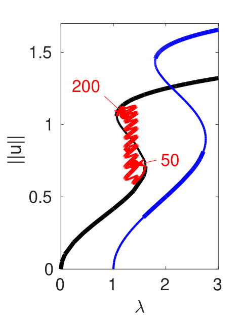 Figure 15
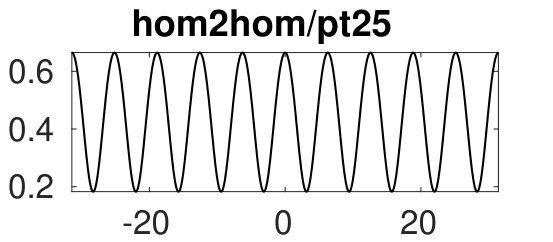 Figure 16
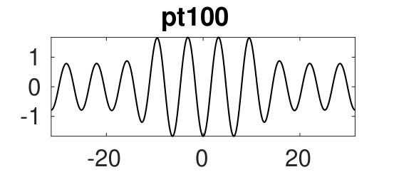 Figure 17
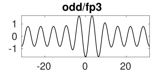 Figure 18
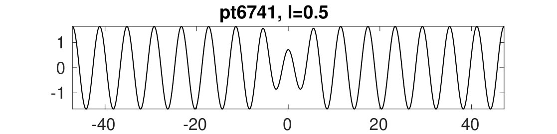 Figure 19
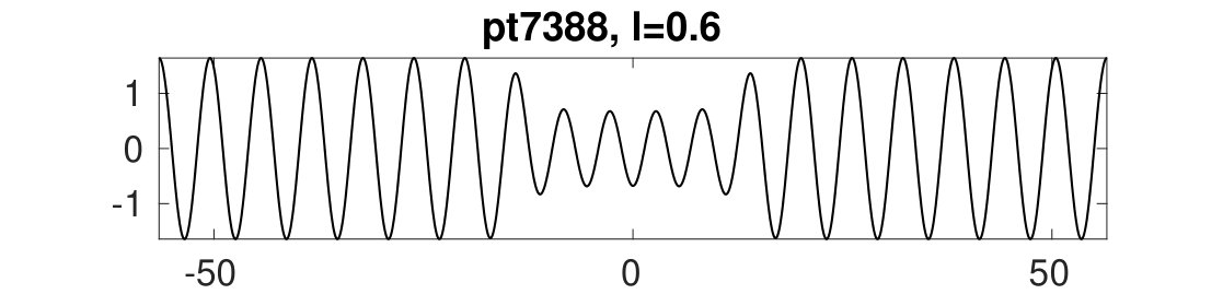 Figure 20
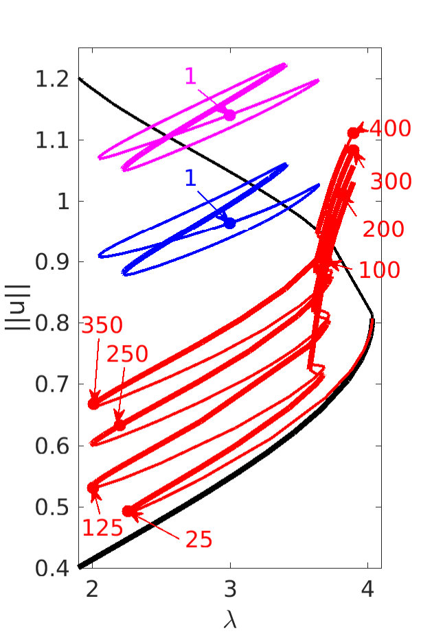 Figure 21
 Figure 22
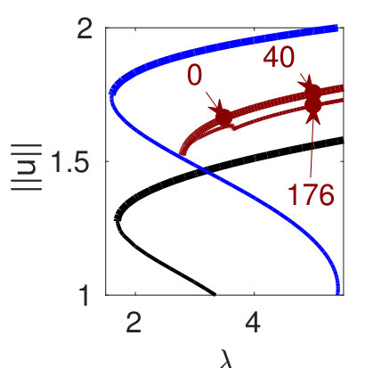 Figure 23
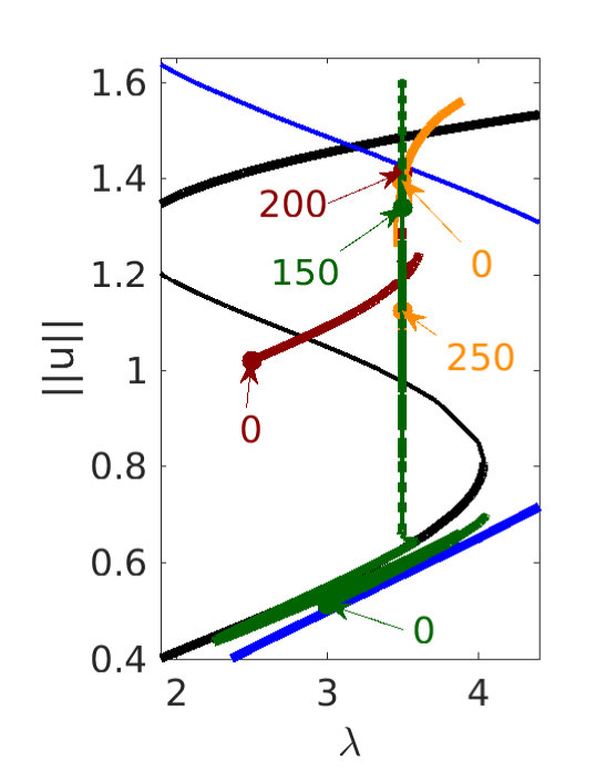 Figure 24
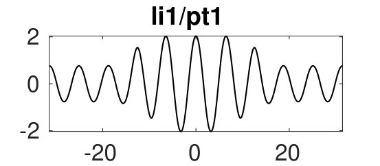 Figure 25
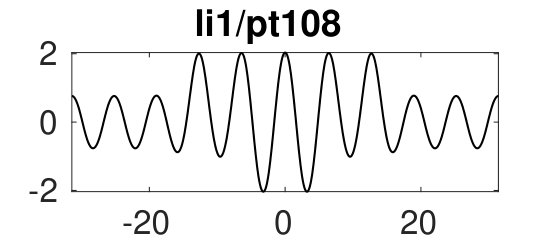 Figure 26
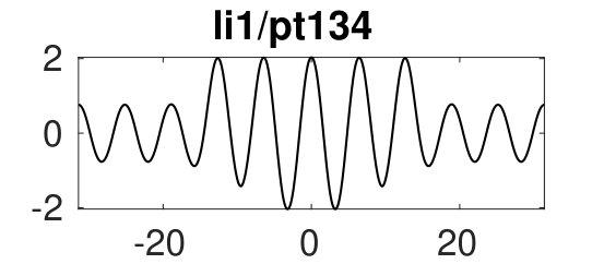 Figure 27
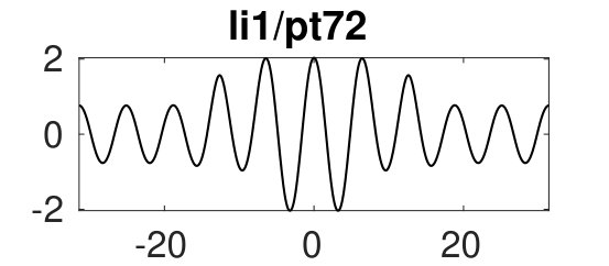 Figure 28
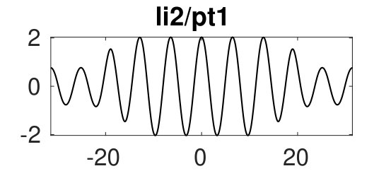 Figure 29
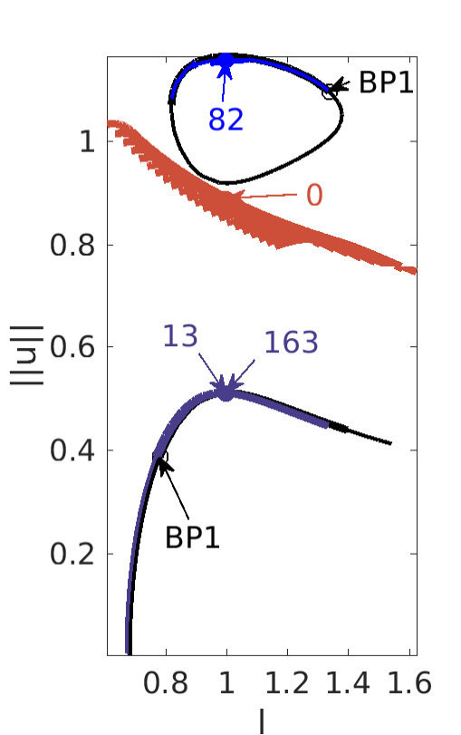 Figure 30
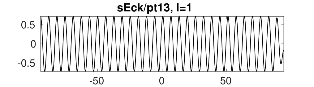 Figure 31
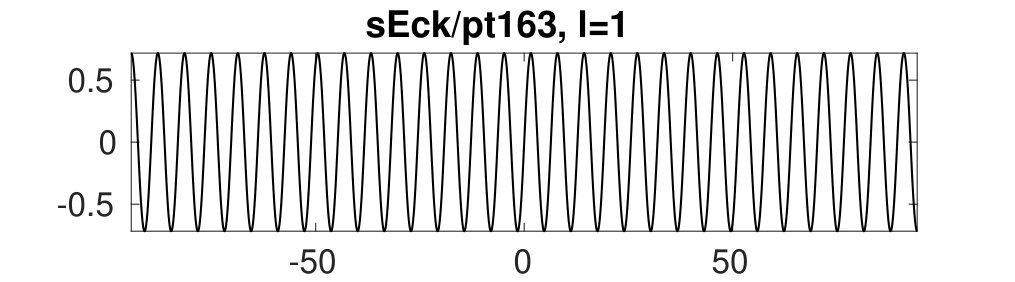 Figure 32
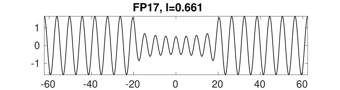 Figure 33
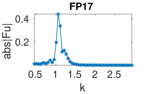 Figure 34
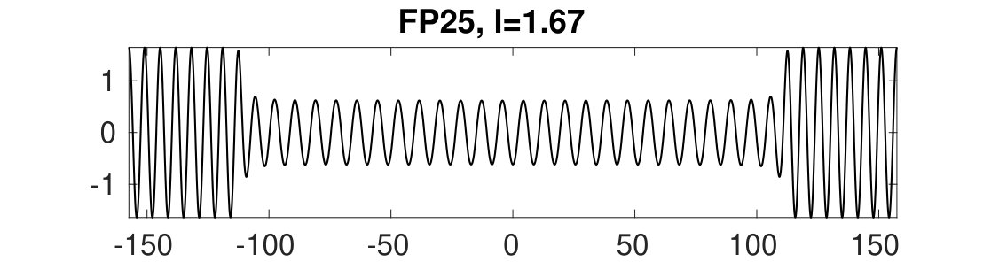 Figure 35
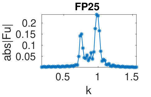 Figure 36
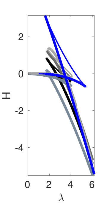 Figure 37
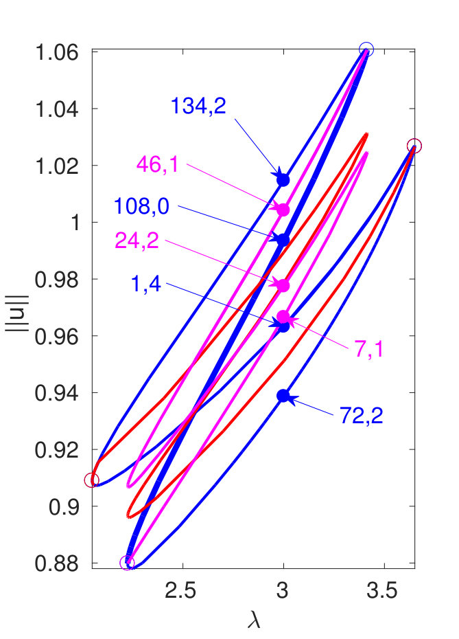 Figure 38
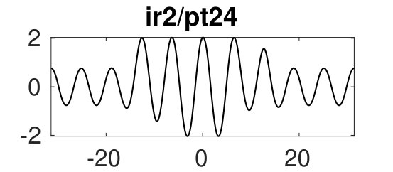 Figure 39
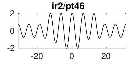 Figure 40
Peer Reviews
No public reviews on file for this paper yet. If you reviewed it on a platform where reviews are public (OpenReview, ICLR, NeurIPS, ICML), you can paste yours below so the community can read it here.
Videos
No videos yet. Explain this paper in a talk, walkthrough, or lecture? Add one.
Defect-like structures and localized patterns in SH357
Edgar Knobloch1, Hannes Uecker2, Daniel Wetzel2 [email protected] 1Department of Physics, University of California, Berkeley, CA 94720, USA
2Institut für Mathematik, Universität Oldenburg, D26111 Oldenburg, Germany
Abstract
We study numerically the cubic-quintic-septic Swift-Hohenberg (SH357) equation on bounded one-dimensional domains. Under appropriate conditions stripes with wave number bifurcate supercritically from the zero state and form S-shaped branches resulting in bistability between small and large amplitude stripes. Within this bistability range we find stationary heteroclinic connections or fronts between small and large amplitude stripes, and demonstrate that the associated spatially localized defect-like structures either snake or fall on isolas. In other parameter regimes we also find heteroclinic connections to spatially homogeneous states, and a multitude of dynamically stable steady states consisting of patches of small and large amplitude stripes with different wave numbers or of spatially homogeneous patches. The SH357 equation is thus extremely rich in the types of patterns it exhibits. Some of the features of the bifurcation diagrams obtained by numerical continuation can be understood using a conserved quantity, the spatial Hamiltonian of the system.
I Introduction
Defects play an important role in both condensed matter physics and in pattern-forming systems. Topological defects arise when the pattern amplitude vanishes and organize both one- and two-dimensional patterns ch93 ; pismen06 . As a result their motion and creation or annihilation lead to nonlocal adjustment of the pattern wave number. Nontopological defects may involve a continuous but spatially localized transition from one wave number to another, and such transitions are usually referred to as fronts ch93 ; pismen06 . Fronts connecting distinct states are common in systems supporting waves as exemplified by the complex Ginzburg-Landau equation huber ; tpk ; motter and pattern formation in fluid dynamics spina and chemistry epstein , and are found in both wave-supporting systems and in stationary patterns. A mathematical classification of defects in one spatial dimension is provided in Ref. scheel .
In this paper we are interested in properties of stationary fronts between patterns with distinct wave numbers in one spatial dimension – the simplest defect – and ask two basic questions. Do such defects come in distinct families and do they persist over time? The first question is motivated by the notion of pinning pomeau whereby a front is pinned to heterogeneities on either side of the front which can be viewed as trapping the front in a particular location. Energy has to be supplied to overcome the resulting pinning potential to move the defect to a different location. The second question has to do with stability of a front. A front may lose stability because of the loss of stability of either of the far-field states or due to a localized mode at the location of the front. These instabilities are usually associated with the presence of unstable continuous and point spectra, respectively. We remark that the classical amplitude-phase description of patterns misses the pinning effect just described since it reduces a uniform pattern to a constant amplitude state and hence treats such states as translation-invariant states. To study fronts between different wave numbers it is essential therefore to go beyond the amplitude-phase description.
The fact that defects are spatially localized structures and that such structures readily pin to heterogeneities suggests that they might come in families organized within a snaking bifurcation diagram. In the context of pattern-forming systems the term homoclinic snaking refers to a pair of intertwined branches of spatially localized patterns that oscillate back and forth across a region in parameter space (the snaking or pinning region), usually accompanied by repeated changes in stability. Prototypes for this scenario in one spatial dimension (1D) are provided by the quadratic-cubic (SH23) and cubic-quintic (SH35) Swift-Hohenberg equations. These take the form
[TABLE]
with and , respectively, and are parametrized by the parameters and . See, e.g., burke ; bukno2007 ; BKLS09 ; bbkm2008 ; dawes08 ; dawes09 ; KAC09 ; hokno2009 ; SU17 for basic properties of these equations and their interpretation. In higher dimensions the situation becomes more complicated, but snaking behavior of branches of localized patterns can also be observed. Snaking of localized hexagons in SH23 and related equations is discussed in, e.g., hexsnake ; w18 , while snaking of localized patterns in 2D reaction-diffusion systems on nonhomogeneous backgrounds is considered in schnaki , and of body-centered cubes on homogeneous and nonhomogeneous backgrounds in 3D reaction diffusion systems in w16 ; UW18b . Refs. kno2008 ; kno2015 provide reviews of localization and snaking in various other systems and experiments, while Refs. chapk09 ; dean11 ; deWitt19 give analytical results on homoclinic snaking based on beyond all orders asymptotics.
Motivated by the above considerations we focus here on 1D patterns but consider a more complex nonlinearity than hitherto studied, in order to study snaking between two distinct periodic patterns. For this purpose we selected the cubic-quintic-septic (SH357) version of (1), namely
[TABLE]
and study this equation on bounded domains with homogeneous Neumann boundary conditions (BCs) . The linear stability properties of the trivial solution are independent of and follow from the linearization . This equation has the solutions , , where . Thus is asymptotically stable for and unstable for with respect to periodic perturbations with wave number near and in 1D we expect pitchfork bifurcations to spatially periodic patterns for , if permitted by the domain and BCs. In detail, if, e.g., , , then the admissible wave numbers are , and for large we have many bifurcation points for small . The first bifurcation at has , and is followed by bifurcations to stripes with , , corresponding to sidebands of .
Depending on the parameters in (2) we find that the bifurcating branches are typically S-shaped, with stable small and stable large amplitude sections, and an unstable intermediate amplitude section. For definiteness, we choose
[TABLE]
and consider as a second free parameter, in addition to . We use the following abbreviations:
- •
for the small amplitude part and for the large amplitude part of the periodic branch belonging to wave number ;
- •
and (without specifying a wave number, but typically with near ) for general periodic solutions;
- •
and for the spatially homogeneous branch (wave number ), bifurcating at ;
- •
, or for the corresponding middle sections.
Figure 1 provides an overview of the dependence of the solution sets of (2) on , and introduces the solution types considered in this paper. Thick lines indicate linearly stable states while thin lines correspond to linearly unstable states. For and not too large the S-shape of the first bifurcating branch is mild, and the subsequent branches are ’neatly ordered’ in the sense that only a short interval of the small amplitude periodic solutions is stable, and there is no overlap of the bistable range of the periodic solutions with wave number near 1 with the branch of spatially homogeneous solutions (wave number ) [Fig. 1(a) for ]. If we increase , the S-shape and hence the overlap of the bistable ranges for solutions with different become more pronounced [Fig. 1(b) for ]. This overlap is of interest to us because we expect localized patterns to be generically present within such bistable (or indeed multistable) ra nges.
It turns out that for the smaller one finds ’almost classical’ snaking of localized states that is associated with heteroclinic cycles between with wave numbers close to , and , again with wave numbers close to . These states consist of a portion of in a background of or vice versa; localized states consisting of a portion of in background are also possible. For larger , more and more branches (with wave numbers deviating from ) enter the game, including the branch of spatially homogeneous solutions (), and the solution set of (2) becomes more and more complicated. For instance, the snaking branches of small–to–large periodic patterns break up into isolas, and additional branches consisting of heteroclinic cycles between various distinct spatial patterns enter the picture. Figure 1 is thus intended as a preview of the subsequent results. The norm used in (a) and all similar plots is
[TABLE]
In summary, in this paper we numerically investigate how the set of localized patterns of (2) becomes richer and richer with increasing , and literally ’explodes’ for and larger. These results are presented in detail in §II, while §III provides a brief discussion.
Remark I.1**.**
(a) Equation (2) has a number of symmetries: (i) translational invariance (for ); (ii) odd symmetry ; (iii) spatial reflection symmetry . The translational invariance (i) is broken over by the Neumann BCs , but “periodic” solutions over can be extended to all of by reflection at the boundaries. Thus the first ’front’ in Fig. 1(a) can also be seen as heteroclinic cycle between a large amplitude and a small amplitude periodic solution. (ii) implies that all nontrivial solutions are double, and we generally identify , , and , respectively. (ii) and (iii) together imply that we have branches of odd solutions of the form , as opposed to even solutions which have a maximum or minimum at . As a consequence, snaking branches come in odd and even families, and generally we expect ladder branches connecting these, and this snakes–and–ladders structure is a prerequisite for the breakup of snakes into isolas. These results are common to SH35 burkeK .
(b) Equation (2) is a gradient system, , with respect to the energy
[TABLE]
, where either , or with Neumann BCs . In particular, local minima of are stable stationary solutions of (2), and (2) does not have time–periodic solutions (with finite energy). Moreover, the translational invariance of yields the existence of a spatially conserved quantity for steady solutions, a spatial Hamiltonian, cf., e.g., (strsnake, , Proposition 1), here given by
[TABLE]
Hence, a necessary condition for a heteroclinic connection between, e.g., two periodic solutions and is that . For the classical SH23 and SH35 equations, this requirement provides an important wave number selection principle that determines the wave number along the snaking branches. The same is true for SH357. Figure 1(e) indicates that while for small to moderate values of there are few intersections of for the different branches, this is no longer so for larger where the number of possible heteroclinic cycles becomes very large.
(c) When choosing the bounded domain for Equation (2) we need to compromise between
Generality: the results should be representative of the situation on large domains, ideally approximating the case ; this in general calls for large domains. 2. 2.
Feasibility and clarity: the domain should be small enough to (i) avoid exceedingly expensive numerics, and (ii) allow clear plotting of results.
It turns out that the basic results can be studied and presented well on relatively small domains, for instance , which we use in most cases. In some cases, in particular for extracting wave numbers from mixed periodic solutions via Fourier transform, a larger such as is helpful. In any case, we checked that none of our results depends qualitatively on the domain size by running the same numerics on significantly larger domains, where however the results become more difficult to present graphically.
(d) For the plots of bifurcation diagrams (BDs) and sample solutions we use the following conventions. Stable parts of branches (as determined from the eigenvalues of the linearization around solutions) are plotted as thick lines, unstable parts as thinner lines. Dots labeled by an integer correspond to solutions for which we plot profiles , titled “pt” if there is no ambiguity. Fold and branch points are indicated via FP and BP, respectively, and similarly in the title of the sample plots. Occasionally we give titles in the form branch/point.
(e) When the spatial dynamics picture implies that is a saddle for with two stable and two unstable eigenvalues. Likewise, a robust connection to or require these to be generalized saddles and hence that they have a three-dimensional center-stable manifold and a three-dimensional center-unstable manifold. This is a consequence of spatial reversibility and the conservation of .
II Results
We use pde2path p2p ; p2phome to compute bifurcation diagrams for (2). As domain we typically choose , which is large enough to permit a multitude of patterns, cf. Remark I.1(c).
II.1 The case
We start with . In the plot of as a function of in Fig. 1(a) we see that there are few self-intersections for the first four bifurcating branches, and in particular no overlap of their bistable ranges with the spatially homogeneous (blue) branch. This corresponds to the ’easy’ situation where relatively few heteroclinic connections are possible. Moreover, in this case transitions between different heteroclinic cycles and interesting codimension two points can be easily identified.
Figure 2 provides more details. In particular, we find that after the first fold on there are multiple BPs where branches of heteroclinic cycles with an increasing number of interfaces bifurcate. The first branch corresponds to fronts (but see also Remark I.1(a) for the interpretation of the front as a heteroclinic cycle via even parity continuation of the solution over the domain boundary), the second to a heteroclinic cycle, and so on. In the following we concentrate on the second (pulse-like) branch for moderate values of but a particular feature of the small regime is clearly visible on the first branch: for , connects to the trivial state , while for it connects to . In other words, each time passes through into the hole in the solution fills in with small amplitude oscillations. On an infinite domain the heteroclinic cycle changes from one involving the state to one involving . Note that there will be parameter values such that the right folds of the snaking front branch just reach , a situation corresponding to a codimension two bifurcation of heteroclinic cycles. There is a second codimension two transition that is relevant as well: when changes from subcritical to supercritical the termination point of the localized solutions moves from to the right fold on as in Fig. 2(a). An analogous transition has been observed in rotating plane Couette flow SGS19 .
The front solutions bifurcate from BP1, the branching point nearest to the right fold of ; other branching points, further away from the fold, give rise to solutions with multiple interfaces, as summarized in Fig. 2(c,d).
II.2 The case
II.2.1 Snakes and ladders of cycles between and
For , the second (leftmost) fold on is at , and the snakes bifurcating near the first fold lie entirely in the range. The red branch in Fig. 3(b) shows the (even) snake bifurcating at BP2. Looking more closely, one finds secondary bifurcation points near every fold on this branch giving rise to ’rungs’ [brown branches in (c)] connecting to the odd snake [, blue branch in (c)]. This ladder structure becomes important for understanding the breakup of snakes at larger , see §II.3. Additionally, in Fig. 3(b) we plot a branch connecting two Turing bifurcation points on . Note that except for , all nontrivial branches are unstable at bifurcation but many become stable at (small but) finite amplitude.
II.2.2 Continuation in the domain size
Along the snaking branches of, e.g., heteroclinic cycles, the wavelengths (and hence amplitudes) of both and must in general change continuously as determined by the condition . Here we look into this phenomenon in more detail, via continuation in the domain size scaling . Thus we modify (1) to
[TABLE]
on , such that the effective domain is . Qualitative results are:
- (a)
In general, is more rigid than . This means that adapts its wave number and amplitude less than does.
- (b)
The continuation in leads to a new kind of snaking, where the small amplitude part of the heteroclinic cycles grows or shrinks via phase slips in .
These results are illustrated in Figs. 4 and 5. Here, to accurately extract the wave numbers of the periodic patterns we choose a rather large base domain , although the phenomenon can be observed on significantly smaller domains, e.g., .
In Fig. 4 we show the results of continuing the periodic branches and in for both increasing and decreasing , starting from results computed earlier for and , and keeping fixed. For decreasing , [lower black branch in Fig. 4(a)] loses stability at corresponding to an Eckhaus boundary point for with wavelength . The bifurcating branch sEck initiates an amplitude modulation at the right domain boundary leading to an increase in the pattern wavelength. With increasing this branch reconnects with the branch near . In the displayed numerical continuation, this manifests itself in ’branch jumping’ to with the corresponding , which we deliberately do not attempt to avoid here by refining the numerics. Instead, we simply continue the branch so found back towards smaller , and find that this branch, like the original branch, also loses stability near . This process can then be repeated. See (b) for sample solution profiles. We emphasize that the continuation of in maintains the number of wavelengths in the domain. Thus the number of wavelengths in a solution can only change by encountering an Eckhaus point, i.e., by triggering a (dynamic) phase slip that takes a stable periodic solution with a certain number of wavelengths to a new stable periodic state with a different number of wavelengths kramerz85 .
Similar behavior takes place for as well. With increasing , loses stability at an Eckhaus point at . Shortly thereafter the branch passes through a fold, and altogether we obtain a closed loop of solutions [upper black branch in Fig. 4(a)]. The bifurcation from at again leads to amplitude modulation at the right domain boundary [Fig. 4(c), middle], but in contrast to the case, the bifurcating branch exhibits two folds near before reconnecting to at the left Eckhaus boundary in . See the first two plots in (c) for sample solutions.
Additionally, Fig. 4(a) shows a snaking branch (red) of heteroclinic cycles, starting at (pt0) with a sample profile shown on the bottom right of (c). This snaking in is shown in more detail in Fig. 5. Starting at pt0 and increasing the solutions remain stable up until close to the first fold near . Near this fold a phase slip is initiated. This phase slip is once again associated with the onset of spatial modulation. This time it is located in the middle of the domain and manifests itself in the splitting of the central peak of the portion of the profile [Fig. 5(b)]. Beyond the fold the new central peak regrows to the amplitude but the solutions are now unstable, and only recover stability at the next fold on the left. The net effect of this process is to add half a wavelength of the state to the solution profile. This process then repeats adding a full wavelength of in the middle of the domain after every two folds, and leading to slanted snaking with increasing . It is clear that these repeated phase slips compress the portion of the solution, although the wavelength of also needs to adapt, albeit only slightly. See the first three plots in (b) for sample profiles. This process continues indefinitely.
If, on the other hand, we start at pt0 and decrease , we can then extend the snake to the left, leading to a shrinkage of the middle section of [see the last plot in (b) for a sample profile]. Panel (d) shows that this shrinkage is in all cases accompanied by significant hysteresis. Panels (d) and (e) show how the above process changes at the left end of the snake. At the leftmost fold [panel (d)], the amplitude of the last remaining peak does not increase to the amplitude. Instead the solution grows new peaks on either side of the central peak thereby initiating a parallel snake similar to that just described, but with all solutions unstable.
To see the wave number adaption in a more quantitative way, in (c) we plot (the (discrete Fourier transform) of the sample solutions from (b). The larger peak, associated to , stays near throughout the snake, while the smaller peak, associated to shifts. In (f) we summarize the wave numbers of the small peaks (red) and of the large peaks (blue) obtained from solutions in the snake. For this we only use solutions for which there is a clear peak separation in Fourier space, and thus solutions with are discarded. The plot shows that adapts much less than . While some scatter due to the limited resolution in Fourier space is present, bands in the wave numbers corresponding to different forward and backward transitions in the snake are clearly visible. Because of the ability of both and states to absorb the wavelength change generated by the phase slips in the center of the domain we conjecture that this type of double structure is more robust with respect to wavelength change than structures that are more rigid.
The above scenario is reminiscent of defect-mediated snaking Ma , with two important differences. In defect-mediated snaking the solution branch appears from a fold on the branch of homogeneous states and so consists of a single branch. Moreover, the snaking is not slanted, because the phase slips do not result in the compression of a second portion of the solution. It is this compression that is in our case responsible for the slanted nature of Fig. 5(a) since it turns the problem into an effectively nonlocal one.
II.3 The case : breakup of snakes into stacks of isolas, and a multitude of cycles
Larger values of result in more and more intersections among for periodic branches with different , and the homogeneous branch [see Fig. 6(a) for ], and thus many more heteroclinic cycles become possible. Up to (say, and depending on the domain size), the basic snake–and–ladders structure from Fig. 3 stays intact, but for larger the snakes and rungs reconnect into a stack of isolas. Moreover, plays an increasing role in the continuation of the solutions. Figures 6(c)-(d) illustrate these effects. The red branch bifurcates from BP1 on , but fails to grow a front between and as it would in ’classical’ snaking at lower . Instead, it now exhibits long, nearly vertical intervals located near , associated first with the growth of a segment of in the solution profile and then its shrinkage before another half period of can be inserted. The branch bifurcating at BP2 on , which at lower generates a snaking branch of heteroclinic cycles, cf. Fig. 3, behaves similarly and also always involves plateaus of .
This type of behavior is similar to that recently found in a Gray-Scott model studied in connection with dryland vegetation patterns where tristability between a pair of different spatially periodic states and a homogeneous state is also present Gandhi2018 , suggesting that the behavior shown in Fig. 6(c) is in fact generic.
On the other hand, we can still generate ’classical’ heteroclinic cycles between and leading to, e.g., the blue and magenta isolas in Fig. 6(c). To generate starting points for these we glue together , segments (using a longer middle segment for the magenta isola) and running a Newton loop to converge to a solution. Figure 7 shows details of the reorganization of the segments that make up the snakes and rungs at smaller into the isola structure.
Figure 6(d) suggests that for we can expect further cycles, not present at small , where the state plays a prominent role. Figure 8 provides some examples. The red branch in (a), with sample solutions in (b), corresponds to heteroclinics. In states of this type it is difficult to eliminate a wavelength of the periodic state in response to parameter changes – it costs less energy to compress the state and expand the homogeneous state or vice versa. Thus phase slips will not be triggered unless the wavelength of the periodic state changes by a substantial amount. Solutions on the lower part of this branch (with pt176) include short loops near and are unstable. Panels (c) and (d) show more heteroclinic cycles, indicating that at large (and on sufficiently large domains) all sorts of connections are possible provided one selects values corresponding to intersections of for the pertinent patterns. We used initial guesses of the form ’pattern-large-to-homogeneous-small’ (pl2hs, red), ’pattern-small-to-homogeneous-small’ (ps2hs, green), ’pattern-small-to-homogeneous-large’ (ps2hl, orange) to converge to the corresponding solutions and continued the resulting solutions to , where they all form localized patterns consisting of (on this domain) up to 4 patches of different solutions (, and ), many of which are stable, albeit in rather narrow intervals. These stability intervals are a consequence of what appears to be collapsed snaking of the corresponding branches in the vicinity of the Maxwell point at . In states of this type changes in the wavelength of the stripe portion of the solution are readily accommodated by changes in the homogeneous portion.
The reconnection of the snaking diagram into a stack of isolas as parameters are varied has been seen in SH23 burke ; BKLS09 and in two-dimensional patterns may even occur as one proceeds up a snaking diagram, all other parameters remaining fixed msand10 ; bramburger .
III Discussion
In suitable parameter regimes, the SH357 equation (2) allows many different heteroclinic cycles between four (recall that we identify and , respectively) main building blocks, namely
and : periodic patterns of small and large amplitude, respectively, with wave numbers near . 2. 2.
and : spatially homogeneous states of small and large amplitude; these can be seen as special cases of and with wave number . However, from the point of view of heteroclinic cycles, the homogeneous states are special in the sense that segments of and can have arbitrary length.
To give some structure to our results, we made the special choice (3), i.e., . For relatively small ( in §II.1), we have a more or less simple situation in the sense that the necessary condition
[TABLE]
for the patterns involved in a heteroclinic cycle only holds for a relatively small number of patterns. Moreover, these values of allow for an interesting continuous transition between heteroclinic cycles between and , and heteroclinic cycles between and . For intermediate ( in §II.2), we obtain ’classical’ snaking of heteroclinic cycles between and . Via continuation in the domain size we also found a new kind of slanted snaking (reminiscent of defect-mediated snaking), where, e.g., the portion of the solution grows or shrinks via phase slips. Finally, for ’large’ , the –– snaking breaks up into stacks of isolas. Moreover, (8) is fulfilled for a large number of different patterns, and consequently many different heteroclinic cycles become possible. In §II.3, we provide several examples of such states for .
In our bifurcation diagrams we indicated linearly stable (unstable) solutions by thick (thin) lines. Owing to the generally large number of different simultaneously stable solutions, periodic and localized, it would be desirable to characterize in addition the different basins of attraction. However, such basins are not yet well understood even for standard homoclinic snaking as described by SH23 or SH35. Therefore, here we confine ourselves to a few remarks: The snakes and related structures such as stacks of isolas typically have rather large basins. For instance the starting points for the computation of the isolas in Fig. 6 can also be obtained from quite rough initial guesses followed by time integration towards a stable solution. Of course, different initial guesses may lead to different but ’nearby’ steady states. Put differently, a localized perturbation of a solution in a snake typically leads to rather fast relaxation either back to , or to a nearby solution in the snake, with, say, one more ’large’ roll and one fewer ’small’ roll. This behavior naturally changes if we go outside the snaking region, or consider delocalized perturbations, which in particular may lead to depinning, as illustrated next.
The states satisfying (8) correspond to time-independent structures (fronts, pulses etc.) and the presence of snaking associated with these connections implies that such structures remain stationary even away from the Maxwell point, i.e., when . If, however, the energy difference between the two competing states becomes too large, the front connecting them depins and the lower energy state invades the higher energy state in a process analogous to depinning of fronts in SH23 or SH35 burke ; burkeK . Figure 9 shows examples of this process, focusing [panels (a-d)] on competition between states that are both spatially periodic, and illustrating possibilities that do not arise in either SH23 or SH35, namely front propagation via repeated phase slips. The fact that phase slips in SH357 can propagate is of particular interest since the Eckhaus instability that triggers them is a steady state instability. Since phase slips require a finite time for proceed to completion we may anticipate the presence of a dynamic regime in which the speed of the front is determined by the phase-slip timescale and not the energy difference alone MaK . In (a), with in the snaking region of Fig. 3, these phase slips adjust the wavelength of the small amplitude portion, but the front between and the resulting from these phase slips remains pinned. In (b) we have two fronts: a fast front consisting of propagating phase slips in , followed by a slower front whereby the higher amplitude but lower energy state invades the smaller amplitude higher energy state. The speed of this amplitude front is not constant, however, and is strongly affected by the phase slips on the portion. We conjecture that this is a consequence of the fact that the wave number has still not relaxed to its equilibrium value when the amplitude front arrives. In (c), corresponding to a slightly larger than in (b), the amplitude front triggers further phase slips, locally accelerating the front and resulting in a type of stick-slip motion at large times. This does not happen in case (b) even at very long times. Finally, in (d) the large amplitude part of the initial condition is dilated relative to its equilibrium wavelength and in this case the system relaxes to a lower energy state via phase diffusion in both and , instead of phase slips. Here the front remains pinned but its location adjusts accordingly.
Figure 9(e) shows a multifront at larger . Here we obtain a –– double front with retreating , obtained from a step-like initial condition, but as suggested by Fig. 8, all sorts of multifronts are possible via appropriate choice of initial conditions. Fronts between homogeneous states are then generically fast, while fronts involving patterned states are typically substantially slower.
Equations of the 357 form have been considered before, in context of the Ginzburg-Landau equation with real coefficients Bortolozzo . When parametrically forced by a spatially periodic function the homogeneous solutions of this equation become periodic solutions with wavelength equal to the forcing wavelength. The resulting equation thus also exhibits coexistence between different amplitude periodic states, and between periodic states and the homogeneous state. While this equation also reveals the gradual breakup of forced snaking into isolas Champneys the situation is different since the wavelength of the periodic states is imposed by the forcing wavelength with the result that bistability between periodic states with different wavelengths is absent. Nevertheless models of this type indicate that the phenomena described here may also occur in periodically forced systems exhibiting periodic states with an intrinsic wavelength. Such systems remain to be studied in detail, although preliminary studies of the spatially forced Swift-Hohenberg equations SH23 and SH35 indicate that the snaking behavior is likewise destroyed as the forcing amplitude increases Kao .
In summary, the SH357 equation is an extremely rich pattern-forming system and may be seen as a one-dimensional model for studying intricate structures in systems exhibiting competition between states with distinct wavelengths. The gradient structure of this equation, and in particular the existence of the spatial invariant , allow a more detailed understanding of the behavior of this equation than is possible for other equations exhibiting similar behavior, such as the Gray-Scott model Gandhi2018 , but neither property is essential for the behavior described here as is well documented for standard homoclinic snaking kno2015 . In particular, standard homoclinic snaking, as described by SH23 or SH35, is robust with respect to both parameter changes and boundary conditions 111In the presence of nonperiodic or non-Neumann boundary conditions an extended periodic state is absent and the snaking localized states turn continuously into a spatially extended state satisfying the boundary conditions mbak2009 ., and for these reasons is found in more complex systems including the equations of hydrodynamics.
Acknowledgment. The work of EK was supported in part by the National Science Foundation under Grant No. DMS–1613132. The work of DW was supported by the DFG under Grant No. 264671738.
The reference list from the paper itself. Each links out to its DOI / PubMed record.
- 1(1) M. C. Cross and P. C. Hohenberg. Pattern formation outside equilibrium. Rev. Mod. Phys. , 65:854–1190, 1993.
- 2(2) L. M. Pismen. Patterns and Interfaces in Dissipative Dynamics . Springer, 2006.
- 3(3) T. Bohr, G. Huber and E. Ott. The structure of spiral-domain patterns and shocks in the 2D complex Ginzburg-Landau equation. Physica D , 106:95–112, 1997.
- 4(4) S. Tobias, M. R. E. Proctor and E. Knobloch. Convective and absolute instabilities of fluid flows in finite geometry. Physica D , 113:43–72, 1998.
- 5(5) Z. G. Nicolaou, H. Riecke and A. E. Motter. Chimera states in continuous media: Existence and distinctness. Phys. Rev. Lett. , 119:244101, 2017.
- 6(6) A. Spina, J. Toomre and E. Knobloch. Confined states in large aspect ratio thermosolutal convection. Phys. Rev. E , 57:524–545, 1998.
- 7(7) I. R. Epstein and J. A. Pojman. An Introduction to Nonlinear Chemical Dynamics: Oscillations, Waves, Patterns, and Chaos . Oxford, 1998.
- 8(8) B. Sandstede and A. Scheel. Defects in oscillatory media: toward a classification. SIAM J. Appl. Dyn. Syst. , 3:1–68, 2004.