Deformed AdS4-Reissner-Nordstr\"om black branes and shear viscosity-to-entropy density ratio
A. J. Ferreira-Martins, P. Meert, R. da Rocha

TL;DR
This paper derives a family of deformed AdS4-Reissner-Nordstr"om black branes, analyzes their properties, and computes the shear viscosity-to-entropy ratio to explore implications for holographic duality and tidal charge constraints.
Contribution
It introduces a new class of deformed black branes using the ADM formalism and applies AdS/CFT methods to determine their shear viscosity-to-entropy ratios.
Findings
New range for tidal charge derived from viscosity ratio
Identification of free parameter values affecting horizon properties
Shear viscosity-to-entropy ratio computed for deformed black branes
Abstract
A family of deformed AdS4-Reissner-Nordstr\"om black branes, governed by a free parameter, is derived using the ADM formalism, in the context of the membrane paradigm. Their new event horizons, the Hawking temperature and other aspects are scrutinized. AdS/CFT near-horizon methods are then implemented to compute the shear viscosity-to-entropy ratio for the deformed AdS4-Reissner-Nordstr\"om metric. The Killing equation is shown to yield new values for the free parameter and the shear viscosity-to-entropy ratio is used to derive a reliable range for tidal charge.
Click any figure to enlarge with its caption.
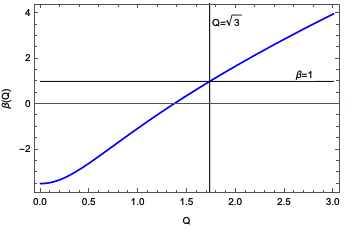 Figure 1
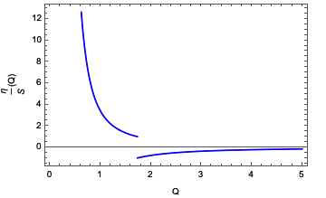 Figure 2
Peer Reviews
No public reviews on file for this paper yet. If you reviewed it on a platform where reviews are public (OpenReview, ICLR, NeurIPS, ICML), you can paste yours below so the community can read it here.
Videos
No videos yet. Explain this paper in a talk, walkthrough, or lecture? Add one.
Deformed AdS4-Reissner-Nordström black branes and shear viscosity-to-entropy density ratio
A. J. Ferreira–Martins
CCCCNH, Universidade Federal do ABC - UFABC, 09210-580, Santo André, Brazil.
P. Meert
CCCCNH, Universidade Federal do ABC - UFABC, 09210-580, Santo André, Brazil.
R. da Rocha
CMCC, Federal University of ABC, 09210-580, Santo André, Brazil.
Abstract
A family of deformed AdS4–Reissner–Nordström black branes, governed by a free parameter, is derived using the ADM formalism, in the context of the membrane paradigm. Their new event horizons, the Hawking temperature and other aspects are scrutinized. AdS/CFT near-horizon methods are then implemented to compute the shear viscosity-to-entropy ratio for the deformed AdS4–Reissner–Nordström metric. The Killing equation is shown to yield new values for the free parameter and the shear viscosity-to-entropy ratio is used to derive a reliable range for tidal charge.
I Introduction
The AdS/CFT correspondence consists of a solid apparatus where strongly coupled QFTs can be studied. Any given QFT, including finite temperature ones, has a hydrodynamical description in the infra-red (IR) limit, corresponding to long length scales in the theory. In the anti-de Sitter (AdS) bulk space, a theory of gravity is dual to the CFT on the boundary. The AdS bulk geometry can include a black brane presenting an event horizon. The holographic duality between the AdS bulk and its boundary then conjectures that the CFT at the long scale regime must be ruled by a near-horizon limit regarding dual geometries. For instance, any general relativistic black hole presents a spurious fluid on its horizon, consisting of the so-called membrane paradigm, whose low-energy regime is a strongly coupled field theory malda ; Iqbal:2008by . In the membrane paradigm, black holes were scrutinized Casadio:2015gea ; daRocha:2017cxu , in the long wavelength limit. Transport coefficients were introduced by the duality between black branes in the AdS bulk and fluid dynamics, in the AdS boundary Bhattacharyya:2008jc . In the membrane paradigm, the AdS boundary can be identified with a brane, in the fluid/gravity correspondence structure ssm1 . As a black brane is a solution of the Einstein’s equations in the AdS bulk, the 4D brane can be also taken as an appropriate landscape, where black holes on the brane are also solutions of the Einstein’s effective field equations. However, considering the 4D brane embedded in the AdS bulk, yields the AdS Riemann tensor to be related to the brane Riemann tensor by the Gauss–Codazzi equations. A useful constraint to the Einstein’s effective field equations on the brane ssm1 within the holographic membrane paradigm is to demand the general-relativistic limit, consisting of a rigid brane, meaning a brane that has infinite tension. This condition, in fact, produces a physically correct low-energy limit, allowing the construction of black holes on the brane casadio ; Ovalle:2017fgl ; first ; mgd1 ; mgd2 .
Methods in AdS/CFT and the membrane paradigm were successful derived in Refs. Antoniadis:1998ig ; Antoniadis:1990ew . Tests of AdS/CFT have been performed in cases for which the supergravity backgrounds are supersymmetric Meert:2018qzk ; Bonora:2014dfa . However, a static AdS black hole in the supersymmetric limit can have a naked singularity, avoided when rotation is assumed, as in the Reissner–Nordström spacetime. Exploring the precise link between braneworld scenarios and the AdS/CFT duality, realized through the membrane paradigm ads_memb , provides a transliteration of the brane models into the AdS/CFT language. It allows to scrutinize black branes and their hydrodynamics using the well-known AdS/CFT methods. In this work, we shall focus on computing transport coefficients, including the shear viscosity-to-entropy density ratio, . Thereafter, viscosity bounds will be imposed to a generalized black brane. The Reissner–Nordström–AdS (AdS4-RN) spacetime plays a prominent role in this procedure, being widely known in the context of AdS/CMT Davison:2011uk ; Cadoni:2009xm for being dual to a finite temperature CFT describing a conserved charge in the boundary. In fact there is a comprehensive literature regarding this spacetime and the related dual theory, regarding holographic superconductors and strange metals Gubser:2008wv ; Hartnoll:2008kx ; Iqbal:2011in ; Giordano:2018bsf .
We will apply the ADM formalism to derive a family of spacetime solutions, leading into the AdS4-RN in a very specific limit. One calls this spacetime a deformation of AdS4-RN. It is governed by a free parameter in the radial component of the metric. When this parameter equals to unity, the AdS4-RN spacetime is then recovered. Although carrying similar features, the bulk geometry of the new solution is quite different of the standard AdS4-RN one. The first aspect noticed is the appearance of a coordinate singularity, which is in fact an event horizon when certain conditions are met. This opens new possibilities, as the horizon is an important feature when exploring the thermodynamic properties of a black hole. It has, thus, direct consequence in the CFT at the AdS boundary. Second, this spacetime can be derived from an action without matter terms, consisting of a vacuum in AdS/CFT, however with a cosmological constant in an AdS5, wherein AdS4 is embedded. This is a consequence of the formalism implied to obtain the solution, and we use the notation for the charge as mere analogy at this point, since its origin is different and the proper terminology is to call it a tidal charge maartens , i. e., the source for this charge is the curvature of the spacetime itself, which comes from a higher dimensional AdS5 bulk.
By allowing a free parameter in the AdS4-RN metric, we expect to gain more freedom, in the sense that intrinsic features, such as transport coefficients and thermodynamic quantities, can be modelled – or fine tuned – according to experimental evidence to come, or even eventually describe unknown materials in condensed matter.
This paper is organized as follows: in Sect. II the spacetime metric, that we call deformed AdS4-RN , shall be derived and some features considered relevant, such as the new horizon, its associated temperature and conditions for such quantities to be meaningful, are studied. We then proceed to describe the process of implementing perturbations to compute the shear viscosity-to-entropy ratio via the fluid/gravity correspondence in Sect. III. In Sect. IV the AdS/CFT correspondence is briefly reviewed for our purposes and applied for computing the shear viscosity-to-entropy density ratio, associated to the dual theory of the deformed AdS4-RN solution. Finally, concluding remarks and some perspectives for the forthcoming developments regarding this type of solutions are presented in Sect. V.
II Deformed AdS4-Reissner-Nordström spacetime
The AdS4–Reissner–Nordström black hole background represents a charged, asymptotically-AdS black hole solution with a planar horizon, described by coordinates ,
[TABLE]
with
[TABLE]
is a well known solution of the 4D Einstein–Maxwell theory with a cosmological constant , where denotes the black hole charge and represents the event horizon position Davison:2011uk ; Cadoni:2009xm , which is unique, as the black hole is extremal.
The AdS/CFT membrane paradigm can set the 4D brane as the boundary of an AdS5 bulk with cosmological constant related to the vacuum energy density of the boundary. The AdS5 bulk, with electromagnetic field strength, satisfies the Einstein’s equations,
[TABLE]
for
[TABLE]
where . Projecting Eq. (3) on an AdS4 brane, with cosmological constant, and introducing Gaussian coordinates in the bulk, and , one obtains the constraints at :
[TABLE]
where is the Ricci curvature scalar, the brane cosmological constant, and represents the electric part of the Weyl tensor. It mimics a Weyl fluid in the bulk maartens , that illustrates how the brane embedding into the bulk contributes to the brane bending, possible by the finite value of the brane tension Ovalle:2017fgl ; c_o_r_2014 ; Casadio:2016aum .
For static solutions, Eqs. (5) emulate the Hamiltonian and the momentum constraints Casadio:2001jg , in the ADM formalism. Such constraints play the important role of sorting out admissible field configurations along manifolds of constant Casadio:2001jg . The selected field configurations thus can be propagated out the AdS4 brane, under the residual Einstein’s effective equations (3). The Hamiltonian constraint comprehends a weaker stipulation than the 4D vacuum equations . The parameter is interpreted as a tidal charge maartens .
Applying the ADM formalism to generate a family of deformed AdS4–RN spacetimes, let us start with the metric (1), still considering the temporal components (2),
[TABLE]
If instead one insists on requiring the AdS4-RN with a regular AdS4 horizon, the price to pay is to have something beyond the vacuum in the bulk, as a field strength Davison:2011uk ; Cadoni:2009xm . This is not the case considered here. Considering that only the component is non-zero, one can check that , and also obtain the components of the stress-energy tensor,
[TABLE]
Equivalently, the electromagnetic potential reads , having the chemical potential and the charge density representing its components of expansion near boundary, . At the horizon, , . Hence , in this regime. Here Q denotes the U(1) gauge charge, then , where is the tidal charge.
A family of analytic solutions of the form (6) obtained by relaxing the condition in (1), by fixing either or as in the AdS4-RN and finding the most general solutions for the constraints (5). These solutions will be expressed in terms of the ADM mass and the parameter , which is fixed but arbitrary Abdalla:2009pg . The momentum constraints are identically satisfied by the metric (6) and the Hamiltonian constraint can be written out explicitly in terms of and . Fixing the temporal component (2), the Hamiltonian constraint in the ADM formalism reads
[TABLE]
for
[TABLE]
where denotes a free parameter that governs the deformation. It is free in the sense that its value is not determined a priori, nevertheless it is taken as constant along the calculations. Hence, the solution
[TABLE]
satisfies Eq. (8), once the temporal component is claimed to be the same as the standard AdS4-RN, given by in Eq. (2). Notice that for , the metric (6) is precisely the RN black hole in AdS4 background. From now on will be assumed for the sake of conciseness.
The electromagnetic potential is determined from the Maxwell equations, which simply read
[TABLE]
where is the electromagnetic field strength. As assumed previously , the solution to (11) is given by
[TABLE]
and one can verify that
[TABLE]
which is nothing but Coulomb’s law - the solution for the spherically symmetric case, considered in the Reissner–Nordström scenario. Moreover one can check that
[TABLE]
It is of no surprise that these conditions are met, since those are the boundary conditions applied to (11). In particular, expansion (15) at the boundary allows to obtain the chemical potential, , of the CFT at the boundary. Explicitly, expanding (12) gives
[TABLE]
The essential features involving the event horizon of AdS4-RN are present in the solution (6). A closer look on (10) reveals that , i.e. , for
[TABLE]
Of course, this is a coordinate singularity at this point, but in fact one can ask weather it if is an event horizon or not. If so, by inspection, it is obvious that leads to , which means that (17) is a bigger horizon than the standard AdS4-RN outer horizon. Hence, it should be considered as the surface for which quantities, such as temperature and entropy of the black hole, are evaluated.
For a static space-time a sufficient condition for a surface to be an event horizon is that it be a Killing horizon wald , which satisfies , where is the time-like Killing vector. Demanding that associated to (10) satisfies such condition, two values of are found:
[TABLE]
As expected, is a solution, which simply confirms that the deformed AdS4-RN contains the standard AdS4-RN, for the previous established value of the deformation parameter. On the other hand, expression (19) fixes according to the value of , which is proportional to the charge placed inside the event horizon when modelling the AdS4-RN spacetime. Eq. (19) is not an intuitive function to picture, hence it is more useful to present its plot and point out certain features, useful for future arguments. Interestingly, it is seen that for both values, (18) and (19), is a Killing horizon and, as was previously established, is a parameter that is not fixed a priori. Moreover, Fig. 1 shows that the range implies , which is the region where (17), with given by (19), should replace for calculations regarding the horizon.
The temperature of this black hole at the horizon is an important quantity, that will be computed according to the geometric procedure outlined in Ref. wald . Such calculation proceeds as follows: one evaluates the quantity
[TABLE]
Then one identifies as the surface gravity by arguing that the computation of such quantity leads to the same expression at the horizon. Then once one has the Killing vector, it is just a matter of computation. It is worth mentioning that Eq. (20) is only valid at , or at any other horizon if such surface exists. However, it cannot be used for other points in spacetime wald . The surface gravity and temperature are closely related by
[TABLE]
Evaluating (20) is fairly simple, and one finds immediately
[TABLE]
Hence, the temperature is identically zero. Notice that this result does not depend on the value of , thus it is valid in the particular choice of given by (19). Moreover, we emphasize that this result is indeed expected, as we are considering an extremal black hole Zaanen:2015oix .
III Fluid/gravity preliminaries
This section is devoted to describe the theoretical background necessary to the computation of the shear viscosity-to-entropy density ratio, usually denoted by , for the deformed RN-AdS4 solutions.
III.1 Linear response theory and Kubo’s formula
Let one consider a theory described by an action . It is often of interest to determine what is the response of a given operator , denoted by , when one adds a coupled external source, . Hence, the theory is altered as son_hydro . The response is determined by employing the linear response theory, establishing that
[TABLE]
where denotes the ensemble average (one-point function) of the operator in the presence of the external source. The method is implemented by applying the time-dependent perturbation theory of quantum mechanics son_hydro ; natsuume , which yields the response, in momentum space,
[TABLE]
where is the Fourier-transformed retarded Green’s function associated to natsuume .
Eq. (24) shows that the response to the operator, by a coupled external source, is narrowed down to the determination of the retarded Green’s function, which is related to a transport coefficient through the Kubo’s formula. Hereon we are ultimately interested in obtaining the shear viscosity as a transport coefficient emerging in the fluid dynamics that is dual to the deformed RN-AdS4 family of solutions.
III.2 Hydrodynamics and fluid dynamics
The formalism of hydrodynamics provides a description of the macroscopic behaviour of a given system. More precisely, it refers to the dynamics of macroscopic variables, with main interest to the conserved ones, that remain in the hydrodynamic limit, characterized by a low-energy, long-wavelength regime natsuume . Thus, from the field theoretical point of view, hydrodynamics is a legitimate effective theory. Therefore, one cannot expect it to carry the details of a microscopic theory, which are encoded in the transport coefficients.
For a simple fluid, one can consider, as a macroscopic variable, the energy-momentum stress tensor, , along with its conservation law, . In dimensions, , a symmetric rank- tensor, has 10 independent components, whilst its conservation law provides only 4 equations. In order to close the equations of motion one must introduce a constitutive equation, which is conveniently written in terms of the normalized fluid velocity field , its rest-frame energy density and its pressure .
In general, one introduces a constitutive equation by determining the form of in a derivative expansion. To first order, dissipation effects, which are absent in the perfect fluid – which corresponds to the zeroth order – are included. A viscous fluid has stress tensor expressed as Rangamani:2009xk
[TABLE]
where the term contains dissipative effects. In the local rest frame, it is such that
[TABLE]
Notice that two transport coefficients are introduced when dissipative effects are considered: the shear, , and bulk, , viscosities. The introduction of a constitutive equation for the viscous fluid closes the equations of motion, yielding the continuity and the Navier–Stokes equations.
III.3 Kubo’s formula for the shear viscosity
General relativity states that spacetime fluctuations bring up fluctuations into the stress tensor wald . In agreement with this idea, the Kubo’s formula for the shear viscosity can be derived by coupling fictitious gravity to the fluid, and then determining the response of , under gravitational perturbations. At this stage, one should see this procedure just as a quick way to derive the Kubo’s formula, as one does not really curve spacetime in fluid experiments. However, the derivation presented here has a natural interpretation within the AdS/CFT duality framework, as discussed in Sec. IV.
First, one adds a gravitational perturbation to a 4D spacetime. Since we are interested in determining the shear viscosity , it is natural to consider an off-diagonal perturbation, so that the perturbed metric is, in the coordinate system, given by
[TABLE]
for
Since the perturbed spacetime is no longer flat, one must extend the constitutive equation for the stress tensor to a curved spacetime, according to
[TABLE]
so that the dissipative part now reads
[TABLE]
where represents the covariant derivative with respect to the perturbed metric . The is the projection tensor, necessary to write the constitutive equation in a covariant way.
Notice that the perturbation is considered to be homogeneous, as well as the fluid velocity field, i.e., . However, parity invariance forbids motion in any direction, so the fluid must be at rest. Therefore, the covariant derivative of the velocity field is reads . Calculating the response in , up to linear order in the perturbation, requires the covariant derivatives . Notice that they are of linear order in the perturbation,
[TABLE]
so that the terms proportional to in Eq. (29) will be second order in the perturbation. Now, since is already linear in the perturbation, one can use the projection tensor in the rest frame and in flat spacetime, . In fact, considering the perturbed metric contribution yields in terms an order higher in the perturbation. Therefore, the response in reads
[TABLE]
whose Fourier transformation yields
[TABLE]
Comparing Eq. (32) with the general result from linear response theory of Eq. (24), in this case, , one obtains the Kubo’s formula,
[TABLE]
Naturally, does depend neither on nor on , which is why one takes the limit and set in the Green function, accounting to . Of course, the problem of finding the retarded Green’s function remains, and one will employ the AdS/CFT methods to this task.
IV AdS/CFT and the GKP–Witten relation
The core claim of the AdS/CFT duality malda is that the generating functionals, or partition functions, of the gauge and gravitational theories are equivalent, , which is realized through the (Lorentzian) GKP–Witten relation gkp1 ; gkp2 :
[TABLE]
where denotes an ensemble average. The represent a field in the gravitational (bulk) theory, and is the on-shell action. Also, , in coordinates such that the AdS boundary where the gauge theory lives is located at – for the spacetime we are working with, c.f. Eq. (6), one has . Hereon the coordinate will be used instead of , that is, the functions appearing in the metric coefficients (2) and (10) are now and , respectively.
The left-hand side of Eq. (34) is the generating functional of the -dimensional boundary gauge theory, when an external source is added, whilst the right-hand side of Eq. (34) is the generating functional of a -dimensional bulk gravitational theory. The on-shell action is obtained by simply evaluating the integral when the field is the solution of the equations of motion meeting certain conditions imposed at the AdS boundary, . Now, since is the solution of the equation of motion, reduces to a surface term on the AdS boundary, which allows us to obtain from the -dimensional action a -dimensional quantity, which is identified with the generating functional of the boundary theory, according to Eq. (34). This is the sense in which we loosely say that the gauge theory lives on the boundary of the bulk.
An important point to notice is that, from the -dimensional point of view, is a field propagating in the bulk; whilst is an external source from the -dimensional point of view. Therefore, in the context of AdS/CFT, one can say that a bulk field acts as an external source of a boundary operator.
In practice, the greatest operational advantage provided by the GKP–Witten relation is the possibility of obtaining the generating functional of a gauge theory by the evaluation of the classical action of a gravitational theory. As we are interested in the response of a system in the presence of an external source, one obtains, from the GKP–Witten relation, the following expression for the one-point function natsuume ,
[TABLE]
Naturally, to obtain the one-point function in the absence of the external source, one evaluates the expression above for , that is, .
The gravitational theory to be considered is classical 4D general relativity with negative cosmological constant, , i.e., the Einstein–Hilbert action plus a matter term
[TABLE]
where is chosen according to the boundary theory. Besides, as the term can be included into the part , since it does not contribute for the computation of the shear viscosity, . Although it does contribute to the computation of other transport coefficients, as the conductivities, which is not our aim here.
The Here a massless scalar field is considered
[TABLE]
In fact, since one is only interested in the asymptotic behaviour, the metric (6) reads
[TABLE]
which is, of course, the AdS spacetime. In these coordinates the equation of motion from Eq. (37) is
[TABLE]
where the prime denotes differentiation with respect to . Notice that the Einstein–Hilbert action does not play any role in the calculation of , since it is independent of the field . Requiring the scalar field to be static and homogeneous along the boundary direction, , yields
[TABLE]
The usual technique to proceed is integration by parts, leading to
[TABLE]
where it is assumed that the scalar field vanishes at the horizon. The second term in Eq. (41) is just the equation of motion (39), which has the following asymptotic solution
[TABLE]
For a scalar field of this form, Eq. (42), the action (41) reduces to a surface term on the AdS boundary. Substituting (42) on the action and evaluating the surface term, the on-shell action reads
[TABLE]
Thus, the one-point function from (35) is given by
[TABLE]
which, compared to the linear response relation of Eq. (24), yields the Green function:
[TABLE]
IV.1 in the deformed RN-AdS4 black brane
A bulk perturbation can be considered, such that
[TABLE]
where is given by (6). According to the linear response theory, the response in the boundary energy-momentum tensor is given by
[TABLE]
where is the perturbation added to the boundary theory, which is asymptotically related to by
[TABLE]
holding as long as obeys the equation of motion for a massless scalar field natsuume ; son_hydro . Since the asymptotic behaviour of (6) is given by (38), one can directly apply the results discussed in this section, and treat as the 4D bulk scalar field , which acts as an external source of a boundary operator. Thus, Eq. (44) yields
[TABLE]
Comparing Eqs. (47) and (49) implies that
[TABLE]
On the other hand, the entropy density associated to (6) is, according to the area law, given by 111Recall that we are concerned about the horizon given by , c.f. Eq. (17), with given by (19).. Plugging this result into Eq. (50) yields
[TABLE]
One now must find , by solving the equation of motion for the perturbation , which is that of a massless scalar in a 4D background,
[TABLE]
Taking , the perturbation equation reduces to
[TABLE]
Now, by imposing the incoming wave boundary condition near the horizon and the Dirichlet boundary condition at the AdS boundary, and proceeding as outlined in natsuume to incorporate these conditions222Namely: solving Eq. (53) in the limit and afterwards in a power series of up to in the hydrodynamic limit. one arrives at the full solution
[TABLE]
Accordingly, the full time-dependent perturbation is asymptotically given by
[TABLE]
Comparing now Eq. (55) to Eq. (48), and identifying , one promptly obtains
[TABLE]
Thus, substituting the resulting above in Eq. (51) yields
[TABLE]
for \color[rgb]{0,0,0}\chi_{Q}=\left(-7-27Q^{2}+3\sqrt{9+42Q^{2}+81Q^{4}}\right)^{1/3}, where the parameter is written as given by Eq. (19).
The ratio is a positive quantity, since both the shear viscosity and the entropy density are positive. From the plot in Fig. 2, representing Eq. (57), one sees where this condition is met.
Therefore, the following bound for can be obtained
[TABLE]
for the ratio to assume the saturated value kss , as the initial action is Einstein–Hilbert. Notice that, as defined, the tidal charge must be a positive quantity, so that the interval, which also satisfies the bound, was not considered in this result, which is also very interesting, and worthy of further investigation.
V Concluding remarks and perspectives
The membrane paradigm was here used to derive a new family of deformed AdS4–RN black branes. For it, the ADM formalism was employed, assuming the temporal component fixed, and the Hamiltonian constraint implemented a deformation of the AdS4–RN black brane, given by Eqs. (6, 10). The Killing equation for the Killing vector of the deformed AdS4-RN black brane was then solved, yielding the values of the free parameter given by Eqs. (18) and (19). Although Eq. (18) yields the standard AdS4-RN black brane, Eq. (19) presents new solutions, encoding the deformed AdS4-RN black brane free parameter a function of the black brane tidal charge. The Hawking temperature was also computed in Eq. (22). Fluid/gravity methods were then employed for computing the shear viscosity-to-entropy ratio for the deformed AdS4–Reissner–Nordström black branes. This ratio is used to derive a reliable range for the tidal charge as well.
It is worth to emphasize that the value of the deformation parameter, in Eq. (18), does correspond to the standard AdS4–RN black brane, as expected. In fact by exploring some features of the deformation exposed in Sect. II, we found that the deformation parameter is restricted to a precise value, taking us back to the conventional AdS4-RN spacetime, which we see as an argument in favour of the unicity of this solution, whenever the ADM formalism is utilized.
Preliminary numerical analysis provide us with deformations of the AdS4–RN black brane (1, 2) without AdS5 bulk embedding, as an exact solution of a Lee–Wick-like action of gravity, and then more members of the family of deformed AdS4-RN black branes might be taken into account, with free parameter given by Eq. (19). In order to implement it, the value of cannot be conjectured to be equal to , and must be derived for the Lee–Wick-like action. However, up to now we have not concluded these computations, as the machining time employed is awkwardly long. If these calculations can be finally implemented, and if the ratio allows a value , one can therefore apply the deformed AdS4-RN black brane in the context of the AdS/CMT correspondence. In fact, the standard AdS4–RN black brane is already known to describe the strange metals in the holographic duality setup. By promoting the spacetime metric from the standard AdS4–RN black brane, corresponding to the particular value in Eq. (18), to the deformed family (2, 6) studied here, with the parameter given by Eq. (19), we expect to gain freedom in describing such materials. Hence this family of deformed black branes can model a wider class of strange metals and the parameter in Eq. (19) can be then used to compute other transport coefficients, or fine tune quantities already known, like the electric conductivity and the thermal conductivity, for example.
Acknowledgements
AJFM is grateful to FAPESP (Grants No. 2017/13046-0 and No. 2018/00570-5) and to Coordenação de Aperfeiçoamento de Pessoal de Nível Superior - Brazil. The work of PM was financed by CAPES. RdR is grateful to CNPq (Grant No. 303293/2015-2), to FAPESP (Grant No. 2017/18897-8), and to ICTP HE 210-V, for partial financial support.
The reference list from the paper itself. Each links out to its DOI / PubMed record.
- 1(1) Maldacena J M 1999 Int. J. Theor. Phys. 38 1113 [Adv. Theor. Math. Phys. 2 , 231 (1998)] ( Preprint eprint hep-th/9711200)
- 2(2) Iqbal N and Liu H 2009 Phys. Rev. D 79 025023 ( Preprint eprint 0809.3808)
- 3(3) Casadio R, Ovalle J and da Rocha R 2015 Class. Quant. Grav. 32 215020 ( Preprint eprint 1503.02873)
- 4(4) da Rocha R 2017 Phys. Rev. D 95 124017 ( Preprint eprint 1701.00761)
- 5(5) Bhattacharyya S, Hubeny V E, Minwalla S and Rangamani M 2008 JHEP 02 045 ( Preprint eprint 0712.2456)
- 6(6) Shiromizu T, Maeda K i and Sasaki M 2000 Phys. Rev. D 62 024012 ( Preprint eprint gr-qc/9910076)
- 7(7) Casadio R and Ovalle J 2014 Gen. Rel. Grav. 46 1669 ( Preprint eprint 1212.0409)
- 8(8) Ovalle J 2017 Phys. Rev. D 95 104019 ( Preprint eprint 1704.05899)