On the Efficiency of the Iterative Techniques for Solving Incompressible Navier-Stokes Equations
Mohamed Mohsen Ahmed

TL;DR
This paper compares various iterative methods for solving incompressible Navier-Stokes equations, highlighting the multigrid method's superior efficiency in terms of computational time and iteration count.
Contribution
It provides a detailed numerical comparison of multiple iterative techniques, demonstrating the effectiveness of the multigrid method for these equations.
Findings
Multigrid method outperforms other iterative methods in speed.
Multigrid requires fewer iterations to converge.
Jacobi and Gauss-Seidel are less efficient than multigrid.
Abstract
It is well known that the choice of the iterative method is crucial in determining the speed of the converged solution. This article presents a detailed comparison between several iterative techniques for solving incmopressible Navier-Stokes equations. The numerical approaches implemented in the solver include Jacobi, Gauss-Siedel, Successive Over Relaxation, Alternating Direct Implicit and Multigrid methods. The results reveal that multigrid method is the most powerful iterative method among all other methods investigated in terms of the computational time and the number of iterations.
Click any figure to enlarge with its caption.
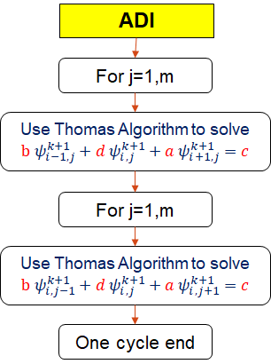 Figure 1
 Figure 2
 Figure 3
 Figure 4
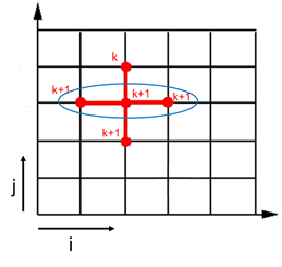 Figure 5
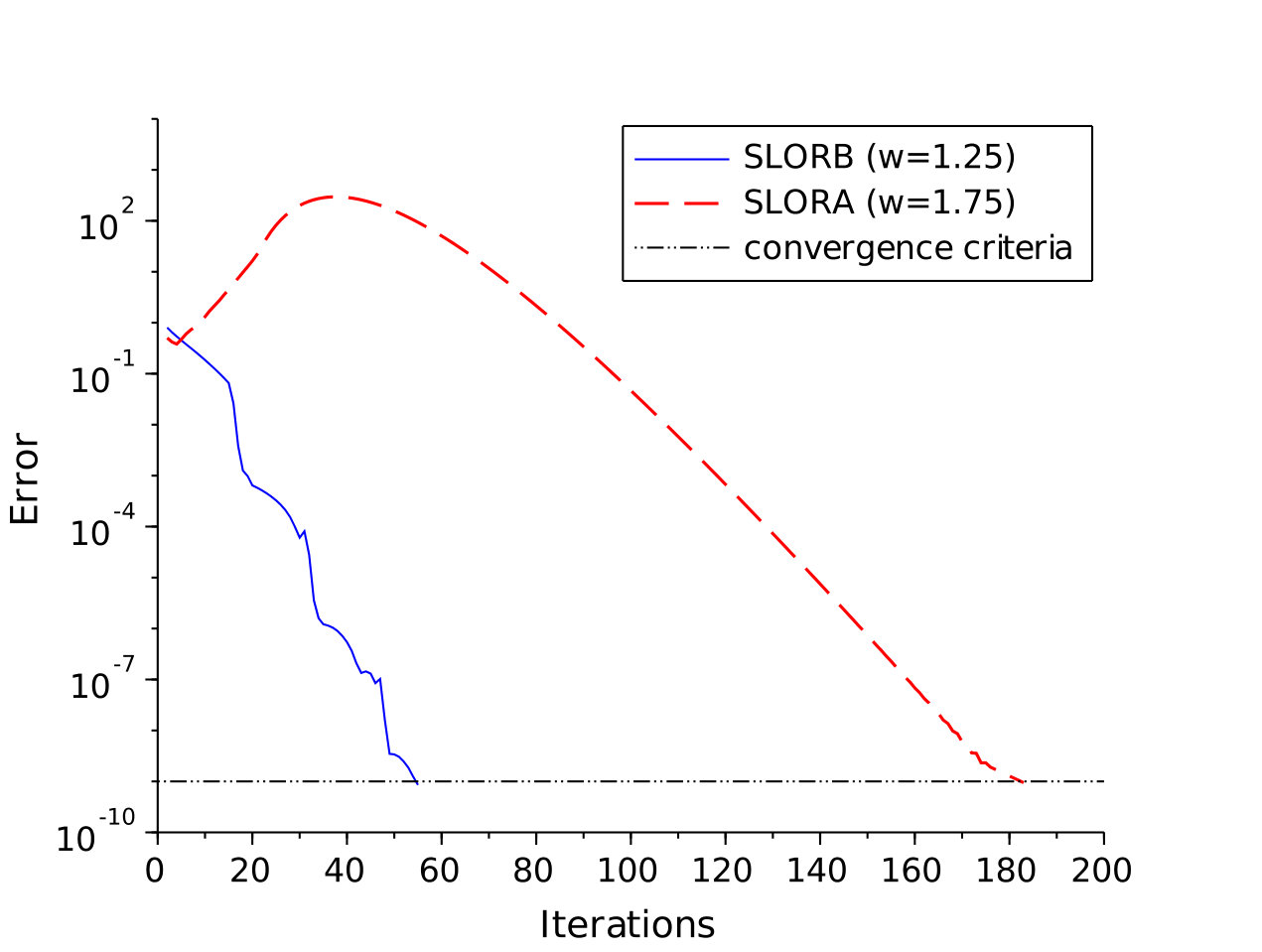 Figure 6
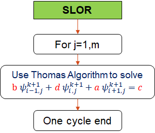 Figure 7
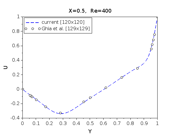 Figure 8
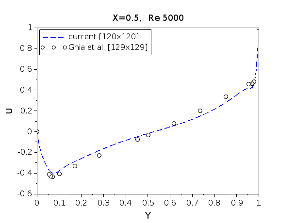 Figure 9
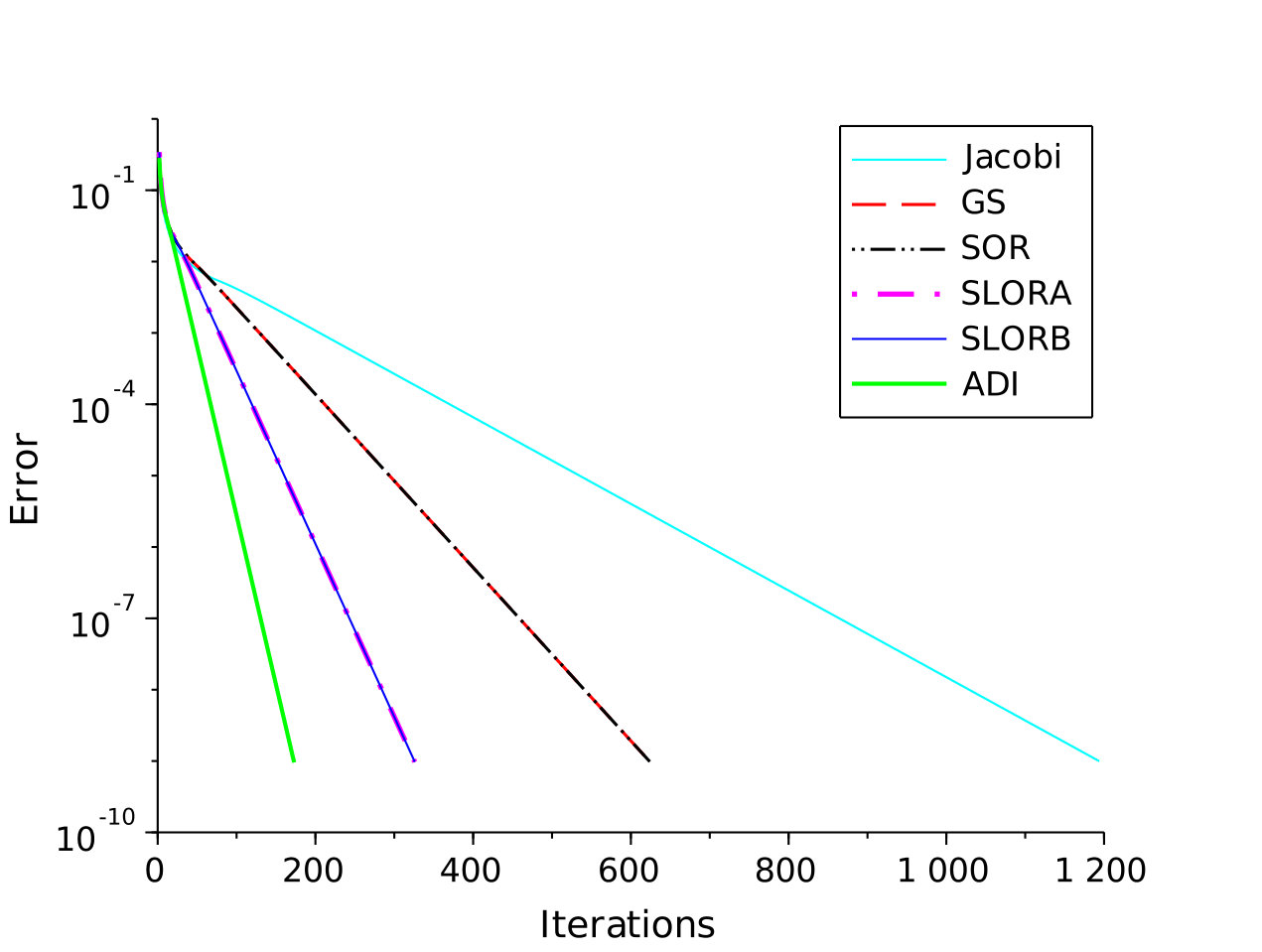 Figure 10
 Figure 11
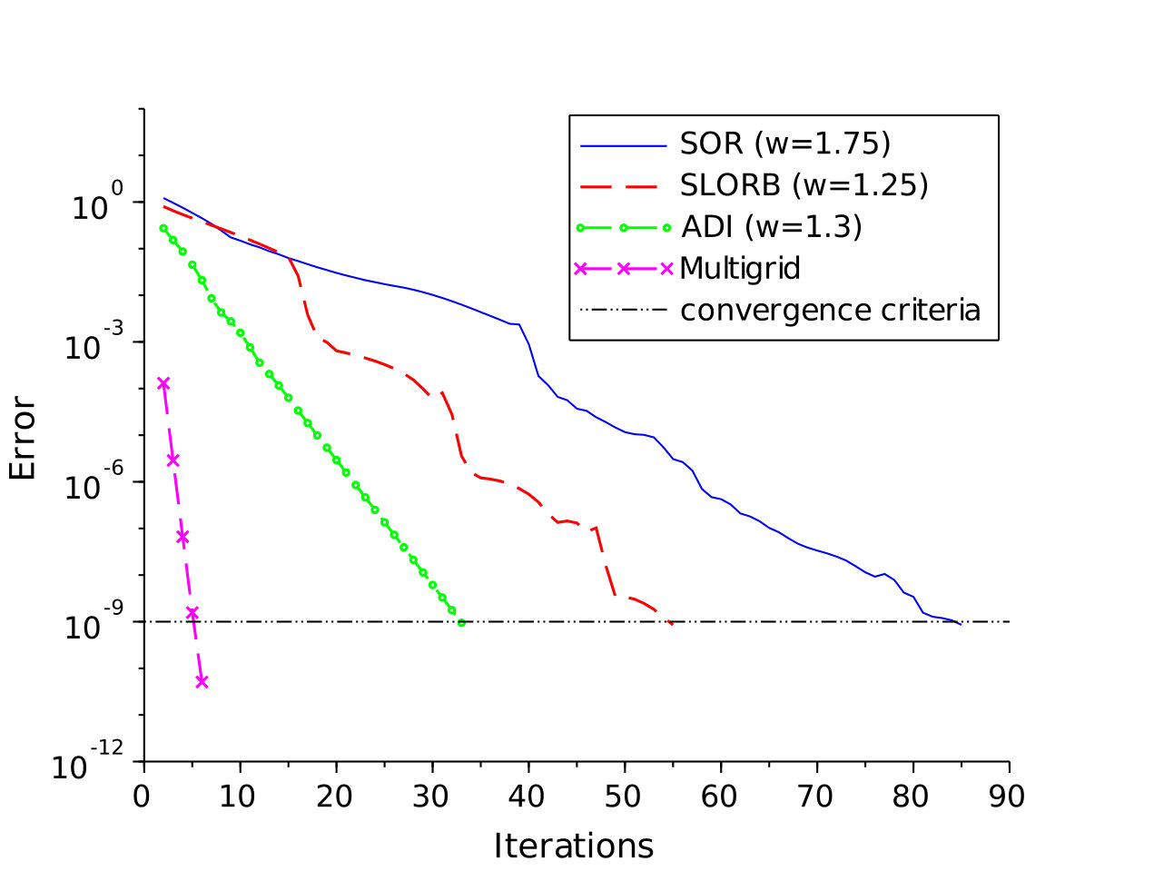 Figure 12
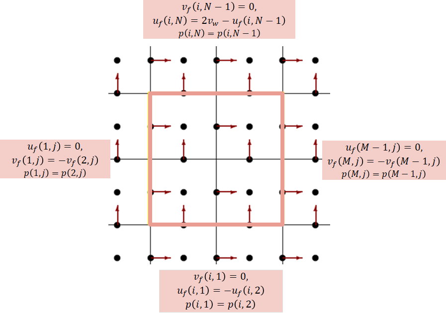 Figure 13
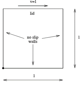 Figure 14
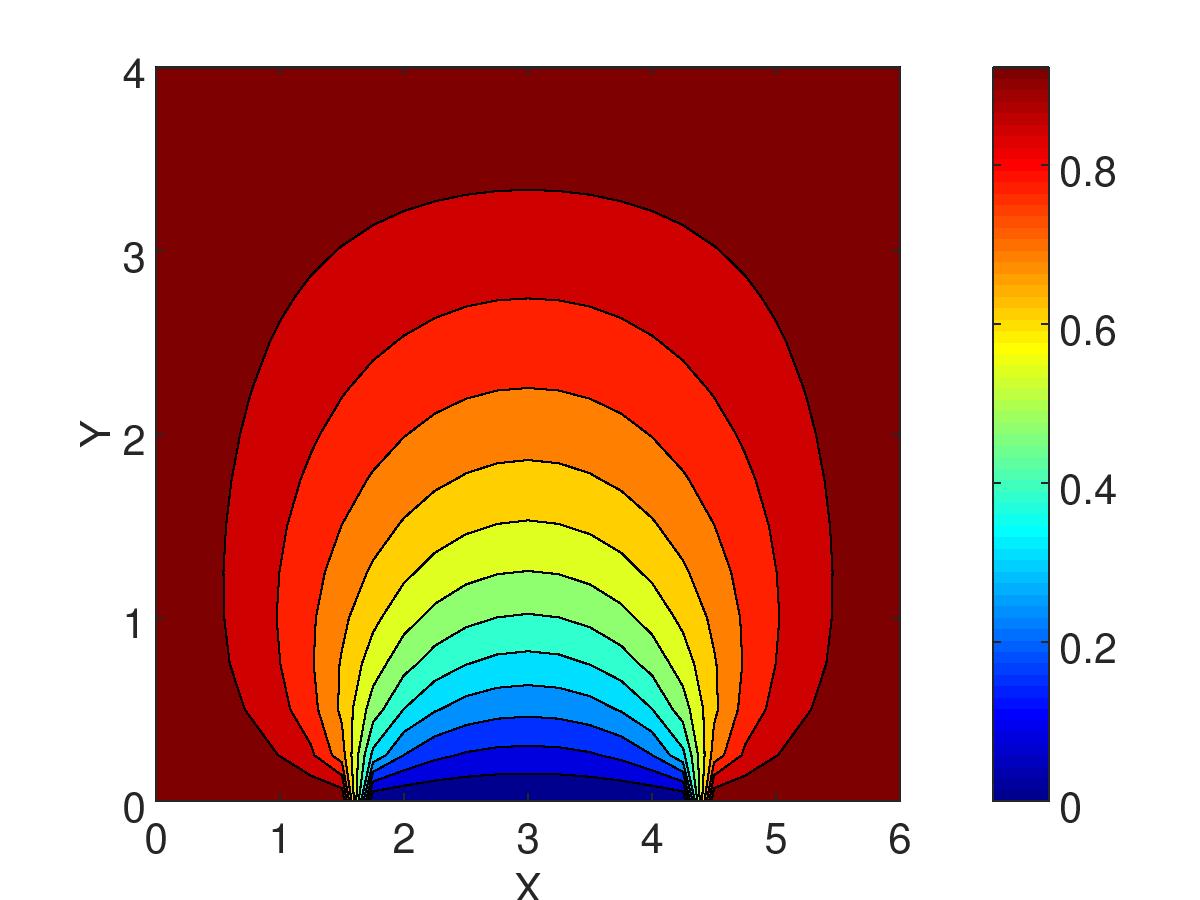 Figure 15
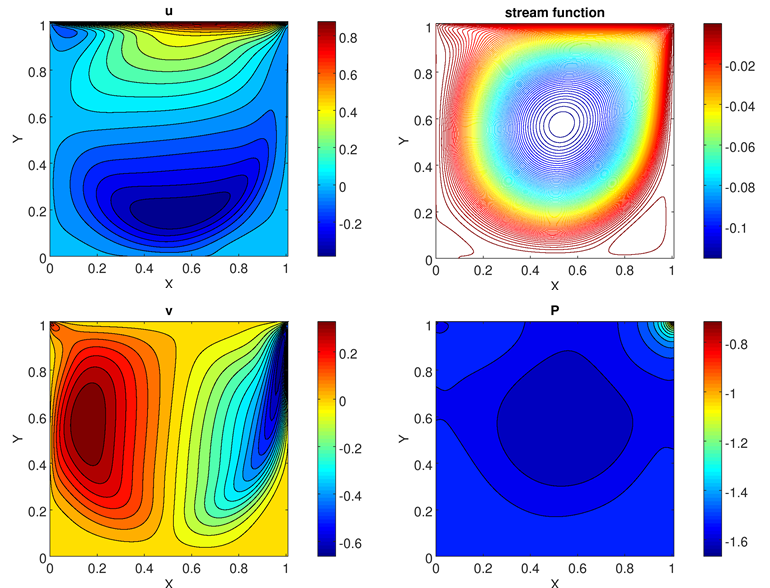 Figure 16
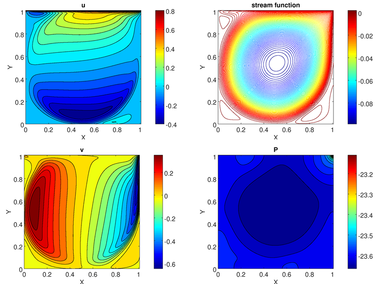 Figure 17
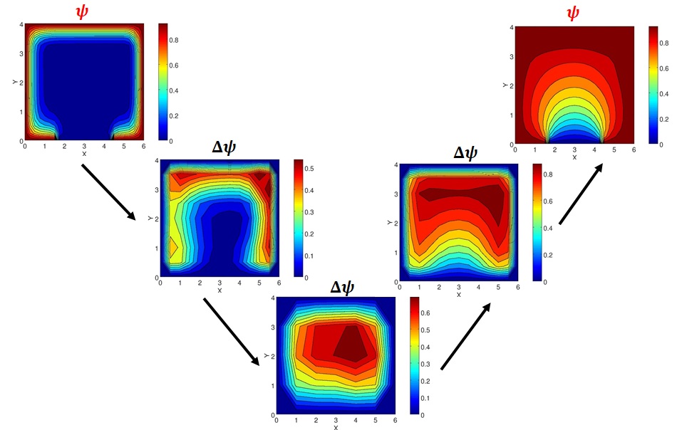 Figure 18
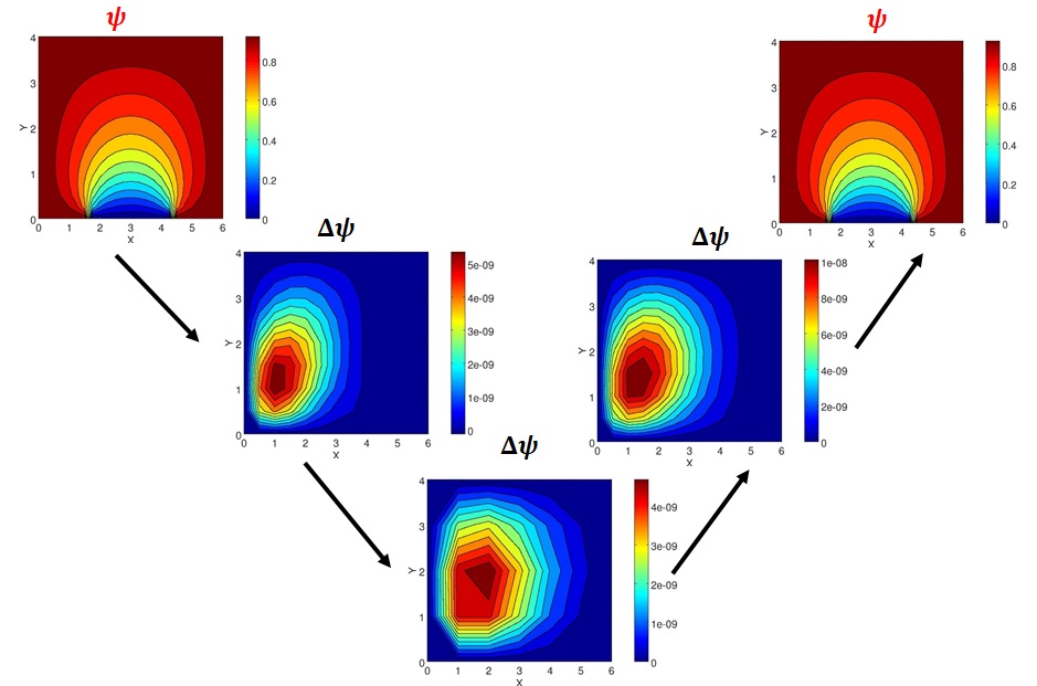 Figure 19
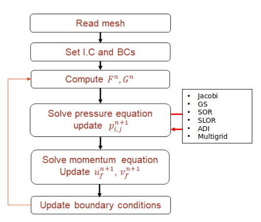 Figure 20
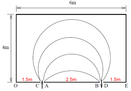 Figure 21
 Figure 22
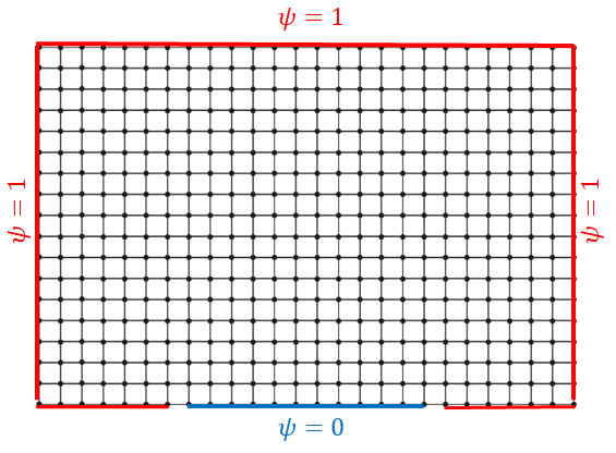 Figure 23
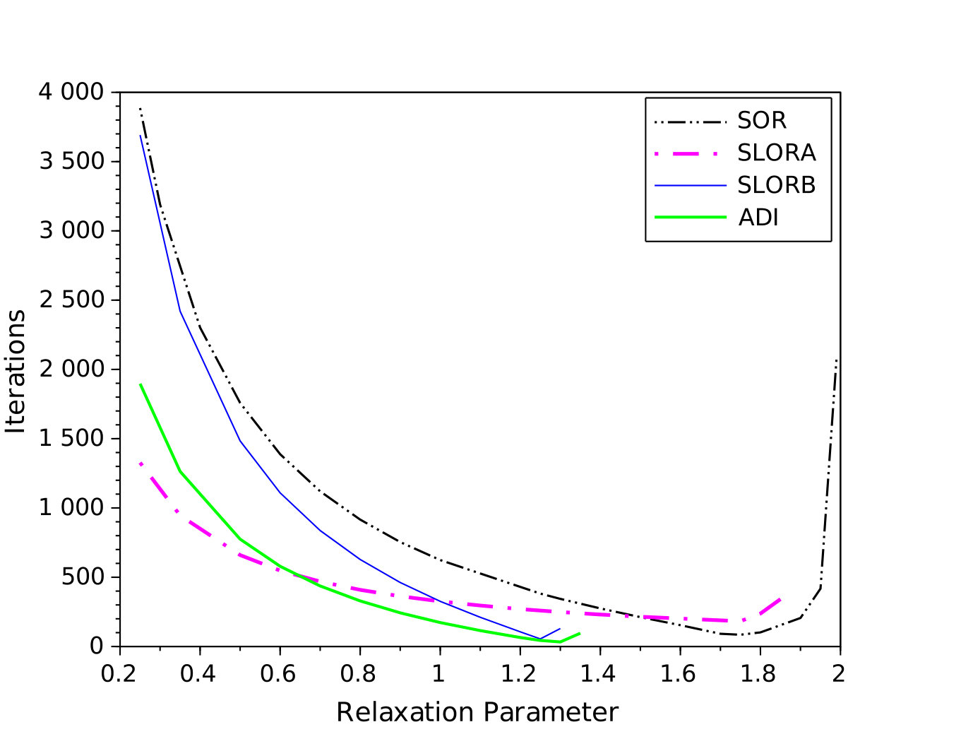 Figure 24
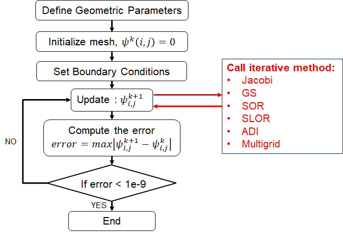 Figure 25
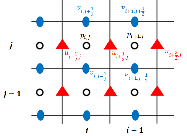 Figure 26
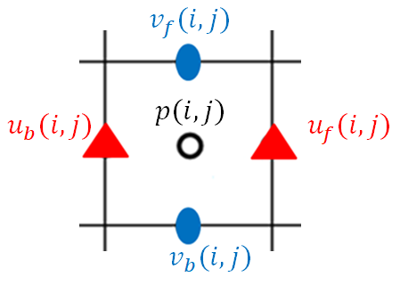 Figure 27
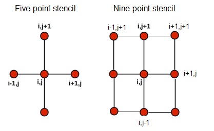 Figure 28
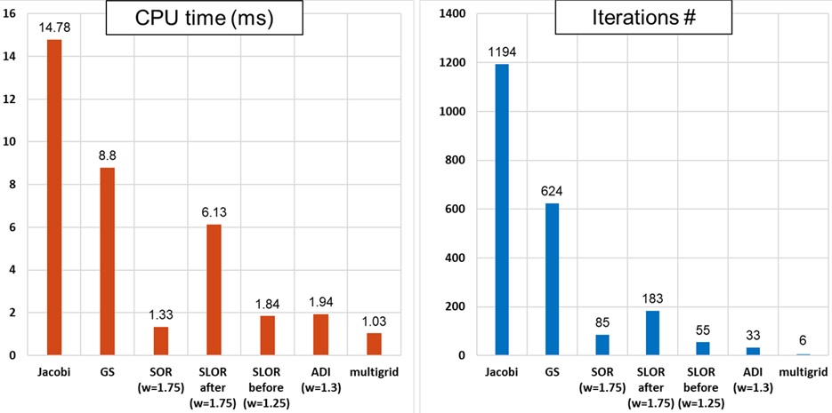 Figure 29
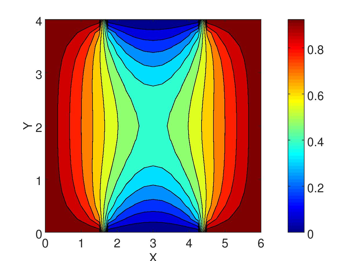 Figure 30
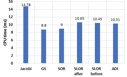 Figure 31
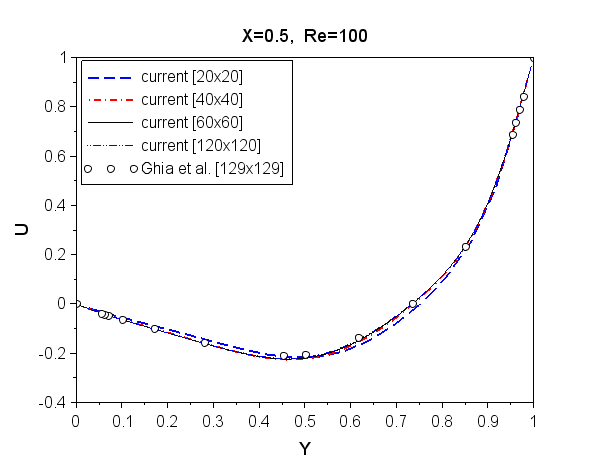 Figure 32
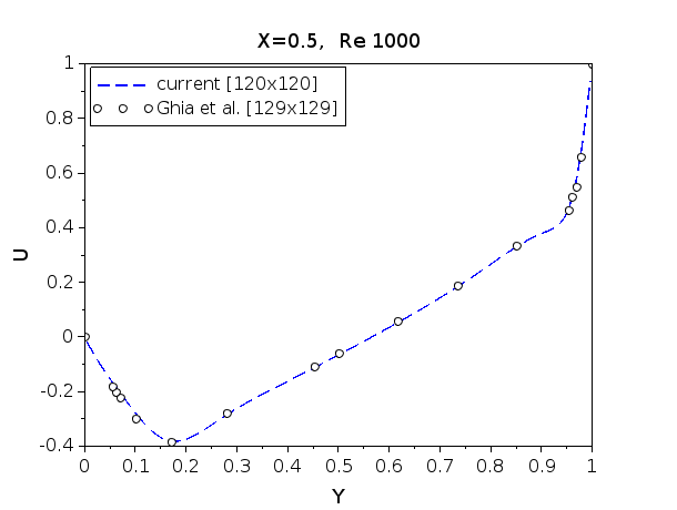 Figure 33
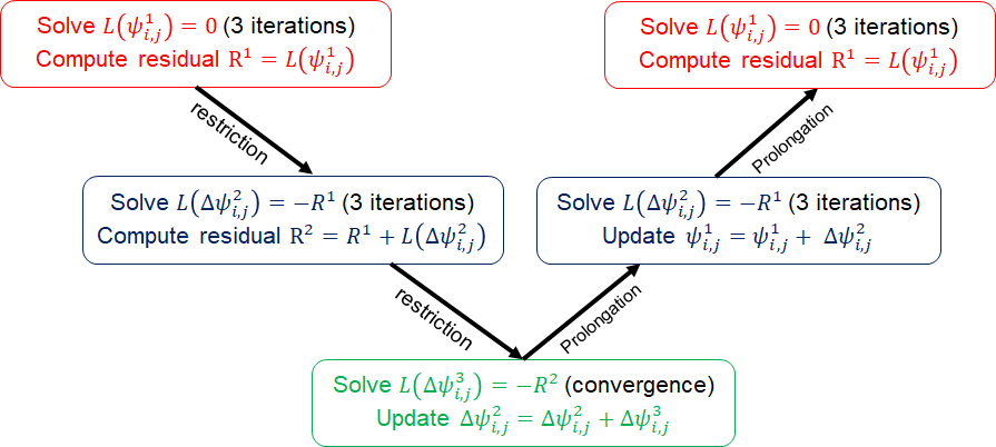 Figure 34
 Figure 35
Peer Reviews
No public reviews on file for this paper yet. If you reviewed it on a platform where reviews are public (OpenReview, ICLR, NeurIPS, ICML), you can paste yours below so the community can read it here.
Videos
No videos yet. Explain this paper in a talk, walkthrough, or lecture? Add one.
Taxonomy
TopicsAdvanced Numerical Methods in Computational Mathematics · Computational Fluid Dynamics and Aerodynamics · Advanced Mathematical Modeling in Engineering
On the Efficiency of the Iterative Techniques for Solving Incompressible Navier-Stokes Equations
Mohamed Mohsen Ahmed111Corresponding author email: [email protected]
Department of Mechanical Engineering, University of Maryland, College Park, Maryland, USA
Abstract
It is well known that the choice of the iterative method is crucial in determining the speed of the converged solution. This article presents a detailed comparison between several iterative techniques for solving incmopressible Navier-Stokes equations. The numerical approaches implemented in the solver include Jacobi, Gauss-Siedel, Successive Over Relaxation, Alternating Direct Implicit and Multigrid methods. The results reveal that multigrid method is the most powerful iterative method among all other methods investigated in terms of the computational time and the number of iterations.
Keywords: Iterative techniques, Elliptic equations, Projection Method, ADI, Multigrid
1 Introduction
Navier-Stokes equations are non-linear second order coupled partial differential equations that an exact solution can only be obtained if certain approximations are performed. Therefore, numerical solutions of Navier-Stokes equations are the most practical method for engineering application involving complex flows. However, complex flows are associated with different length and time scales such that a large number of iterations using a sufficiently large number of grid points or mesh cells should be carried out in order to converge to a solution that captures the complex flow physics. Although parallel computing has been widely used to deal with large number of mesh cells by distributing the mesh on several processors using different decomposition methods [1], the choice of the iterative method that shall be used to solve the governing equations remains crucial in determining the speed of obtain a converged solution.
This paper presents a detailed comparison of the speed of the most common iterative techniques that are employed in solving a system of equations. The iterative techniques employed in this study include Jacobi, Gauss-Siedel (GS), Successive Over Relaxation (SOR), Successive Over Relaxation by Line (SLOR), Alternative Direct Implicit (ADI) and multigrid. The numerical example employed in this study is the solution of the incompressible Navier-Stokes equations using projection method [2].
The governing equations in the non-dimensionalized primitive variable form are
continuity equation
[TABLE] 2. 2.
Momentum equation x-direction
[TABLE] 3. 3.
Momentum equation y-direction
[TABLE]
2 Discretization of the Governing Equations
Finite difference method is employed to discretize the governing equations on a staggered grid. The use of staggered grid allows the coupling between and at adjacent point, thus, preventing oscillations and checker-board effects. In the description of staggered grid, the pressure is defined at the cell center point . However, the velocity components are defined as and which correspond to forward and backward edges of the cell corresponding to point . The velocity at the cell center point is calculated from the average of the forward and backward velocities such that
[TABLE]
The continuity equation can be discretized using central differencing about point as
[TABLE]
Explicit discretization of the x-momentum equation about point using central differences yields
[TABLE]
where
[TABLE]
Similarly, the y-momentum equation is discretized as
[TABLE]
where
[TABLE]
The subscripts and correspond to the corner points of the cell whose center is point . The corresponding terms are
[TABLE]
The pressure Poisson equation is finally obtained from the discretized continuity and momentum equations such that
[TABLE]
where
[TABLE]
Since projection method provides an explicit expression of the momentum equation, limitations are introduced on the maximum time step for a stable solution. Peyret and Taylor [3] provided a correlation between the time step, Reynolds number and mesh size. If the restriction is
[TABLE]
Now we have all equations in a discretized form, the next step is to implement these equations in a FORTRAN code. The overall FORTRAN solver algorithm is explained in the flowchart of figure 1.
3 Results and Discussion
Two test cases are considered. First, a square cavity of unity length with a moving top surface is considered for validation and verification purposes. The top wall is moving with speed and all other walls are not moving. Different grid sizes are considered for each simulated case. Ghost cells are introduced on the staggered grid to specify the constraints of the boundary points. No slip and zero pressure gradient are specified on all walls. A study on the mesh size effect on the solution is performed first at a Reynolds number of 100. A qualitative comparison is carried out between the current solution and two different benchmark solutions by Ghia et al. [4]. Figure 2 shows the distribution of velocity along y-direction at for different mesh levels at when the solution reached steady state (time=17.24 s). It can be inferred that a grid independent solution can be obtained at mesh level 60x60 or above.
The second test case involves flow in the chamber described in figure 4. The inlet and outlet small gaps are . A uniform grid is constructed with constant spacing . The computational grid and boundary condition is provided in figure 1. The total number of grid pints in the domain is 425 points. The simulations are performed on a single processor and the CPU time is recorded for all cases.
All numerical methods are first compared without over relaxation in order to give us confidence on the validity of our solver to predict well known trends. Figure 5 shows the number of iterations and the error of the different iterative methods employed in the solver. The slowest method is Jacobi which requires 1194 iterations to reach convergence. GS and SOR with no relaxation are identical and the number of iterations is 624 iterations, which is approximately half the number of iterations of Jacobi method. SLORB and SLORA, which refer to applying over relaxation before or after each GS line iteration cycle, are much faster than GS and SOR method with only 326 iterations. Although ADI method is the fastest among these methods with only 326 iterations, it should be taken into consideration that two calculations are conducted inside a single cycle of the ADI method. In figure 6, the CPU time for each method is reported. It can be inferred that Jacobi is the slowest method, GS is the fastest method and SLOR and ADI methods are approximately equal in terms of computational time due to the reasons discussed previously.
Now, we are in turn to find the value of the best over relaxation parameter that would speed up the calculations of the SOR, SLOR and ADI methods. Figure 7 show the effect of the relaxation parameter on the number of iterations. It can be seen that there exist an optimum value of and this value is different for different iteration methods. The optimum values of are 1.75, 1.75, 1.25 and 1.3 for SOR, SLORA, SLORB and ADI respectively. Figure 8 shows the error vs. number of iterations required at the best relaxation parameter for each iterative method.
The number of iterations and CPU times for all methods with optimal relaxation are summarized in figure 9. As expected, ADI requires less number of iterations that SLORB (33 vs. 55). However, the total CPU time is almost identical in both cases. Another important observation is that SLORA is much slower than SLORB and SOR with optimal over relaxation parameter. Figure 10 compares SLORB and SLORA at their optimal over relaxation parameters. It is inferred that although is higher in SLORA, more number of iterations is required since the solution overshoots in the first 50 iterations. The only explanation of this observation is low stability of Thomas’ algorithm [5] while solving the tri-diagonal matrix when the matrix is not diagonally dominant.
It is also concluded from figure 9 that multigrid method is the most efficient method among all other iterative methods. The solution converged after only six V-cycles and the total CPU time is around 1.03 milliseconds which is fastest relative to all other methods.
4 Conclusion
Despite the rapid growth in parallel computing, the properties of the iterative methods are the key parameter for determining the speed of obtaining a converged solution on a single processor. Six different implicit and explicit iterative methods were compared while solving a 2-dimensional incompressible Navier-Stokes eqations. The results reveal multigrid method is more efficient that other iterative methods in terms of number of iterations and computational time.
5 Funding
This study was conducted without a funding support.
6 Conflict of interest
The authors declare that there is no conflict of interest.
7 Appendix: Incompressible N-S Equations Fortran Solver
program Incomp_NS
implicit none !!!!!!-------variables declaration--------!!!!! integer :: m,n,i,j, iteration , counter ,anim_freq real(8) :: Lx,Ly,dx,dy,beta, v_w , Ren, cycles ,relaxation real(4) :: time, t_final, dt , CFL real(8),allocatable,dimension(:,:) :: P, u_f, u_b, v_f , v_b , u , v , R , psi , vor real(8),allocatable,dimension(:,:) :: F_f, F_b , G_f, G_b real(8),allocatable,dimension(:,:) :: uv_ff , uv_fb , uv_bf , uv_bb real(8),allocatable,dimension(:,:) :: P_old,P_new, difference real(8) :: max_error , u_center character(len=50) :: filename real(8) :: mm,nn !!!!!-------------Inputs-------------!!!!! cycles=100000 anim_freq=500 Lx=1.0d0 Ly=1.0d0 v_w=1.0d0 m=240 n=240 dx=Lx/(m-2) dy=Ly/(n-2) beta=dx/dy time=0.0d0 Ren=10000.0d0 dt=0.0025Rendx**2 t_final=cycles*dt CFL=dt/dx relaxation=1.3 mm=m nn=n
!!!!!-------Creating variables--------!!!!! allocate(P(m,n) , u(m,n) , v(m,n) , R(m,n) , psi(m,n) , vor(m,n)) allocate(u_f(m,n) , u_b(m,n) , v_f(m,n) , v_b(m,n)) allocate(uv_ff(m,n) , uv_fb(m,n) , uv_bf(m,n) , uv_bb(m,n)) allocate(F_f(m,n), F_b(m,n), G_f(m,n), G_b(m,n)) allocate(P_new(m,n),P_old(m,n),difference(m,n)) P=0.0d0 u=0.0d0 v=0.0d0 R=0.0d0 psi=0.0d0 vor=0.0d0 uv_ff=0.0d0 uv_fb=0.0d0 uv_bf=0.0d0 uv_bb=0.0d0 u_f=0.0d0 u_b=0.0d0 v_f=0.0d0 v_b=0.0d0 F_f=0.0d0 F_b=0.0d0 G_f=0.0d0 G_b=0.0d0 P_old=0.0d0 P_new=0.0d0 !!!!!-------Update Boundary conditions--------!!!!! do i=1,m !bottom v_f(i,1)=0.0d0 u_f(i,1)= -u_f(i,2) P(i,1)=P(i,2) !top v_f(i,n-1)=0.0d0 u_f(i,n)=2*v_w-u_f(i,n-1) P(i,n)=P(i,n-1) end do do j=1,n !left u_f(1,j)=0.0d0 v_f(1,j)= -v_f(2,j) P(1,j)=P(2,j)
    !right
    u_f(m-1,j)=0.0d0
    v_f(m,j)= -v_f(m-1,j)
    P(m,j)=P(m-1,j)
end do
do i=2,m
    do j=1,n
        u_b(i,j)=u_f(i-1,j)
    end do
end do
do i=1,m
    do j=2,n
        v_b(i,j)=v_f(i,j-1)
    end do
end do
do i=1,m
    do j=1,n
        u(i,j)=0.5*(u_f(i,j)+u_b(i,j))
        v(i,j)=0.5*(v_f(i,j)+v_b(i,j))
    end do
end do
!!!!!----------------------------Main Solver------------------------------!!!!! counter=0 write (filename,’(A,I6.6,A)’) "p", counter,".csv" print*,filename
  open(unit=100,file=filename)
  do i=2,m-1
     write(100,*) (P(i,j),’,’, j = 2,n-2), P(i,n-1)
  enddo
  close(unit=100)

  write (filename,’(A,I6.6,A)’) "u", counter,".csv"
  print*,filename
  open(unit=200,file=filename)
  do i=2,m-1
     write(200,*) (u(i,j),’,’, j = 2,n-2), u(i,n-1)
  enddo
  close(unit=200)

  write (filename,’(A,I6.6,A)’) "v", counter,".csv"
  print*,filename
  open(unit=300,file=filename)
  do i=2,m-1
     write(300,*) (v(i,j),’,’, j = 2,n-2), v(i,n-1)
  enddo
  close(unit=300)
open(unit=10,file="Time_U.csv")
do counter=1,cycles
time=time+dt
u_center=u(nint(mm/2),nint(nn/4))
print*, ’*********************************************’
print*,’cycle number =    ’, counter
print*, ’dt= ’,dt
print*, ’dx= ’,dx
print*,’current time =    ’, time
print*,’Courant number =    ’, CFL
print*,’monitoring velocity=  ’, u_center

do i=2,m-1
    do j=2,n-1
        uv_ff(i,j)=0.5*(u_f(i,j)+u_f(i,j+1)) * 0.5*(v_f(i,j)+v_f(i+1,j))
        uv_fb(i,j)=0.5*(u_f(i,j)+u_f(i,j-1)) * 0.5*(v_b(i,j)+v_b(i+1,j))
        uv_bf(i,j)=0.5*(u_b(i,j)+u_b(i,j+1)) * 0.5*(v_f(i,j)+v_f(i-1,j))
        uv_bb(i,j)=0.5*(u_b(i,j-1)+u_b(i,j)) * 0.5*(v_b(i,j)+v_b(i-1,j))
    end do
end do
! Intermediate step (F,G) do i=2,m-1 do j=2,n-1 F_f(i,j)=u_f(i,j) +(dt/(Rendx**2))(u_f(i+1,j)-2u_f(i,j)+u_b(i,j)) & +(dt/(Rendy**2))(u_f(i,j-1)-2u_f(i,j)+u_f(i,j+1)) & -(dt/dx)(u(i+1,j)**2 - u(i,j)**2) & -(dt/dy)(uv_ff(i,j)-uv_fb(i,j))
        G_f(i,j)=v_f(i,j) +(dt/(Ren*dy**2))*(v_f(i+1,j)-2*v_f(i,j)+v_f(i-1,j)) &
                 +(dt/(Ren*dy**2))*(v_f(i,j+1)-2*v_f(i,j)+v_b(i,j)) &
                 -(dt/dx)*(uv_ff(i,j) - uv_bf(i,j)) &
                 -(dt/dy)*(v(i,j+1)**2 - v(i,j)**2)

        F_b(i,j)=u_b(i,j) +(dt/(Ren*dx**2))*(u_f(i,j)-2*u_b(i,j)+u_b(i-1,j)) &
                 +(dt/(Ren*dy**2))*(u_b(i,j-1)-2*u_b(i,j)+u_b(i,j+1)) &
                 -(dt/dx)*(u(i,j)**2 - u(i-1,j)**2) &
                 -(dt/dy)*(uv_bf(i,j)-uv_bb(i,j))

        G_b(i,j)=v_b(i,j) +(dt/(Ren*dy**2))*(v_b(i+1,j)-2*v_b(i,j)+v_b(i-1,j)) &
                 +(dt/(Ren*dy**2))*(v_f(i,j)-2*v_b(i,j)+v_b(i,j-1)) &
                 -(dt/dx)*(uv_fb(i,j) - uv_bb(i,j)) &
                 -(dt/dy)*(v(i,j)**2 - v(i,j-1)**2)

    end do
end do
! Pressure equation do i=1,m do j=1,n R(i,j)=( (F_f(i,j)-F_b(i,j))/dx + (G_f(i,j)-G_b(i,j))/dy ) / dt end do end do
!call an iterative solver
call ADI(P,R,m,n,beta,dx,relaxation)
! Momentum equation do i=2,m-1 do j=2,n-1 u_f(i,j)=F_f(i,j) - dt/dx*(P(i+1,j) - P(i,j)) v_f(i,j)=G_f(i,j) - dt/dy*(P(i,j+1) - P(i,j)) end do end do
!!!!!-------Update Boundary conditions--------!!!!! do i=1,m !bottom v_f(i,1)=0.0d0 u_f(i,1)= -u_f(i,2) P(i,1)=P(i,2)
   !top
   v_f(i,n-1)=0.0d0
   u_f(i,n)=2*v_w-u_f(i,n-1)
   P(i,n)=P(i,n-1)
end do

do j=1,n
    !left
    u_f(1,j)=0.0d0
    v_f(1,j)= -v_f(2,j)
    P(1,j)=P(2,j)

    !right
    u_f(m-1,j)=0.0d0
    v_f(m,j)= -v_f(m-1,j)
    P(m,j)=P(m-1,j)
end do

do i=2,m
    do j=1,n
        u_b(i,j)=u_f(i-1,j)
    end do
end do

do i=1,m
    do j=2,n
        v_b(i,j)=v_f(i,j-1)
    end do
end do

do i=1,m
    do j=1,n
        u(i,j)=0.5*(u_f(i,j)+u_b(i,j))
        v(i,j)=0.5*(v_f(i,j)+v_b(i,j))
    end do
end do
!vorticity calculation
do i=1,m-1
    do j=1,n-1
        psi(i,j)=psi(i-1,j)-dx*(v(i,j))
        vor(i,j)=(v(i+1,j)-v(i,j))/(dx) - (u(i,j+1)-u(i,j))/(dy)
    end do
end do
!Animation output if(mod(counter,anim_freq)==0) then write (filename,’(A,I6.6,A)’) "p", counter,".csv" print*,filename
  open(unit=100,file=filename)
  do i=2,m-1
     write(100,*) (P(i,j),’,’, j = 2,n-2), P(i,n-1)
  enddo
  close(unit=100)

  write (filename,’(A,I6.6,A)’) "u", counter,".csv"
  print*,filename
  open(unit=200,file=filename)
  do i=2,m-1
     write(200,*) (u(i,j),’,’, j = 2,n-2), u(i,n-1)
  enddo
  close(unit=200)

  write (filename,’(A,I6.6,A)’) "v", counter,".csv"
  print*,filename
  open(unit=300,file=filename)
  do i=2,m-1
     write(300,*) (v(i,j),’,’, j = 2,n-2), v(i,n-1)
  enddo
  close(unit=300)
endif
write(10,*) time,’,’, u_center
end do
close(unit=10)
!!!!!-------Output results--------!!!! open(unit=1, file="p.csv") do i=2,m-1 write(1,*) (P(i,j),’,’, j = 2,n-2), P(i,n-1) enddo close(unit=1)
open(unit=2, file="u.csv") do i=2,m-1 write(2,*) (u(i,j),’,’, j = 2,n-2), u(i,n-1) enddo close(unit=2)
open(unit=3, file="v.csv") do i=2,m-1 write(3,*) (v(i,j),’,’, j = 2,n-2), v(i,n-1) enddo close(unit=3)
open(unit=4, file="stream.csv") do i=2,m-1 write(4,*) (psi(i,j),’,’, j = 2,n-2), psi(i,n-1) enddo close(unit=4)
open(unit=5, file="vorticity.csv") do i=2,m-1 write(5,*) (vor(i,j),’,’, j = 2,n-2), vor(i,n-1) enddo close(unit=5)
end program Incomp_NS
The reference list from the paper itself. Each links out to its DOI / PubMed record.
- 1Shang [2014] Shang, Z., “Impact of mesh partitioning methods in CFD for large scale parallel computing,” Computers & Fluids , Vol. 103, 2014, pp. 1–5.
- 2Brown et al. [2001] Brown, D. L., Cortez, R., and Minion, M. L., “Accurate projection methods for the incompressible Navier–Stokes equations,” Journal of computational physics , Vol. 168, No. 2, 2001, pp. 464–499.
- 3Peyret and Taylor [1983] Peyret, R., and Taylor, T. D., Computational methods for fluid flow , Vol. 11, Springer-Verlag, New York, 1983.
- 4Ghia et al. [1982] Ghia, U., Ghia, K. N., and Shin, C., “High-Re solutions for incompressible flow using the Navier-Stokes equations and a multigrid method,” Journal of computational physics , Vol. 48, No. 3, 1982, pp. 387–411.
- 5Thomas [1949] Thomas, L., “Elliptic problems in linear differential equations over a network: Watson scientific computing laboratory,” Columbia Univ., NY , 1949.