On the plane into plane mappings of hydrodynamic type. Parabolic case
B. G. Konopelchenko, G. Ortenzi

TL;DR
This paper investigates singularities in plane-to-plane mappings governed by parabolic hydrodynamic systems, analyzing their hierarchy, types, and regularization methods, with implications for broader parabolic mappings.
Contribution
It introduces a hierarchy of singularities for parabolic two-component systems and discusses their regularization via surface deformations, extending Whitney's approach.
Findings
Flex is the lowest singularity in the hierarchy.
Higher singularities are cusp-type curves $(k+1,k+2)$.
Regularization involves deforming mappings into higher-dimensional surfaces.
Abstract
Singularities of plane into plane mappings described by parabolic two-component systems of quasi-liner partial differential equations of the first order are studied. Impediments arising in the application of the original Whitney's approach to such case are discussed. Hierarchy of singularities is analysed by double-scaling expansion method for the simplest -component Jordan system. It is shown that flex is the lowest singularity while higher singularities are given by curves which are of cusp type for , . Regularization of these singularities by deformation of plane into plane mappings into surface to plane is discussed. Applicability of the proposed approach to other parabolic type mappings is noted.
Click any figure to enlarge with its caption.
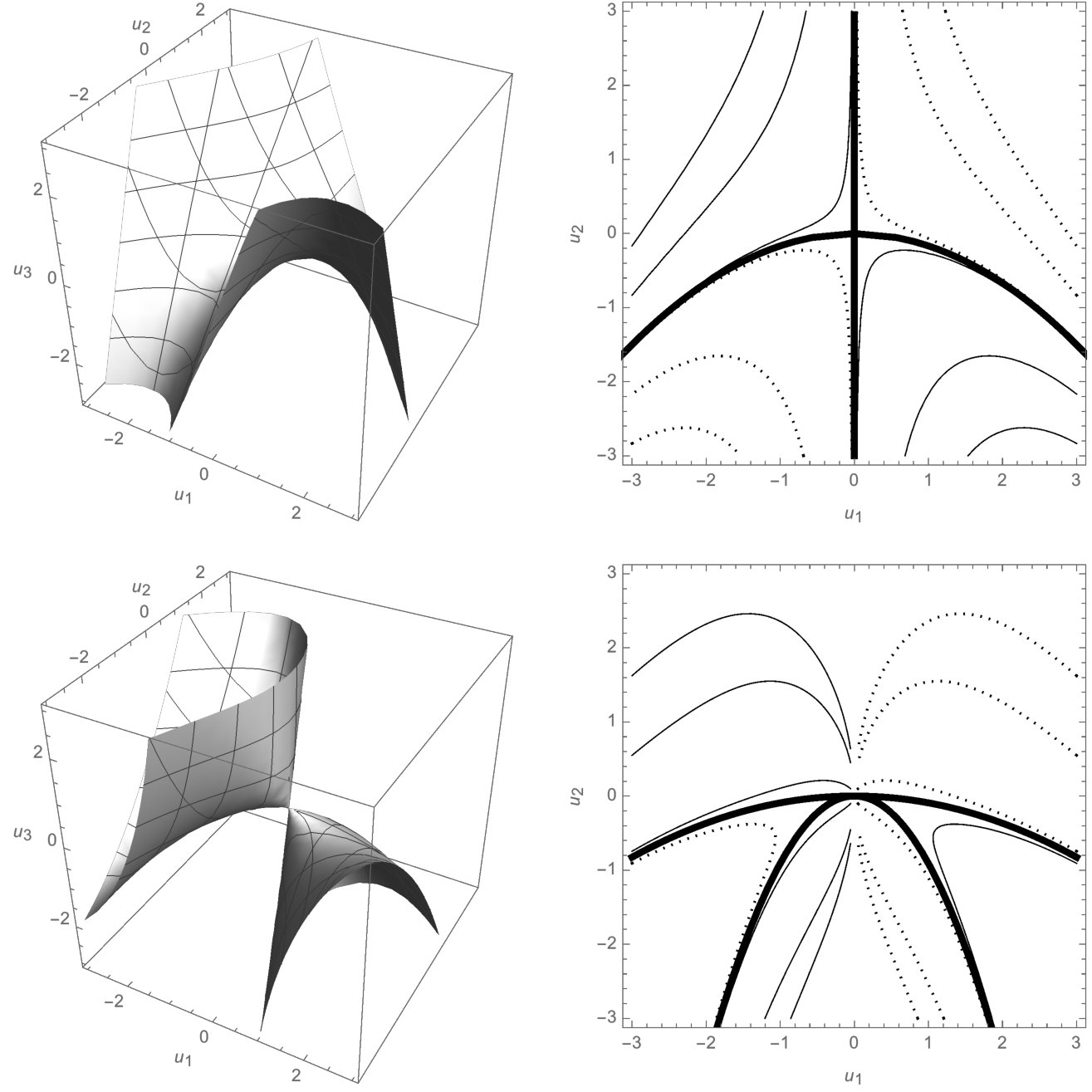 Figure 1
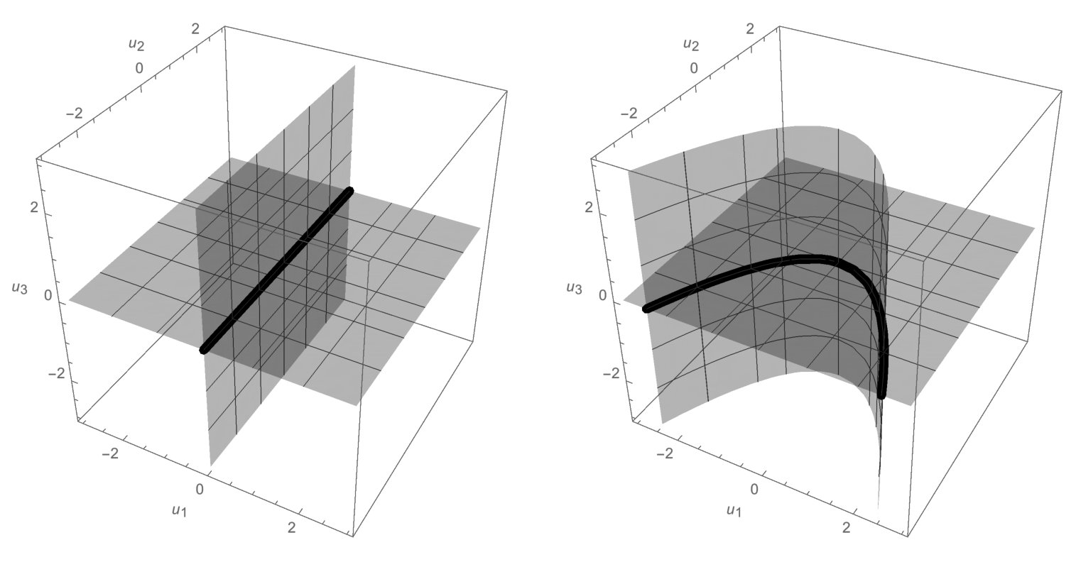 Figure 2
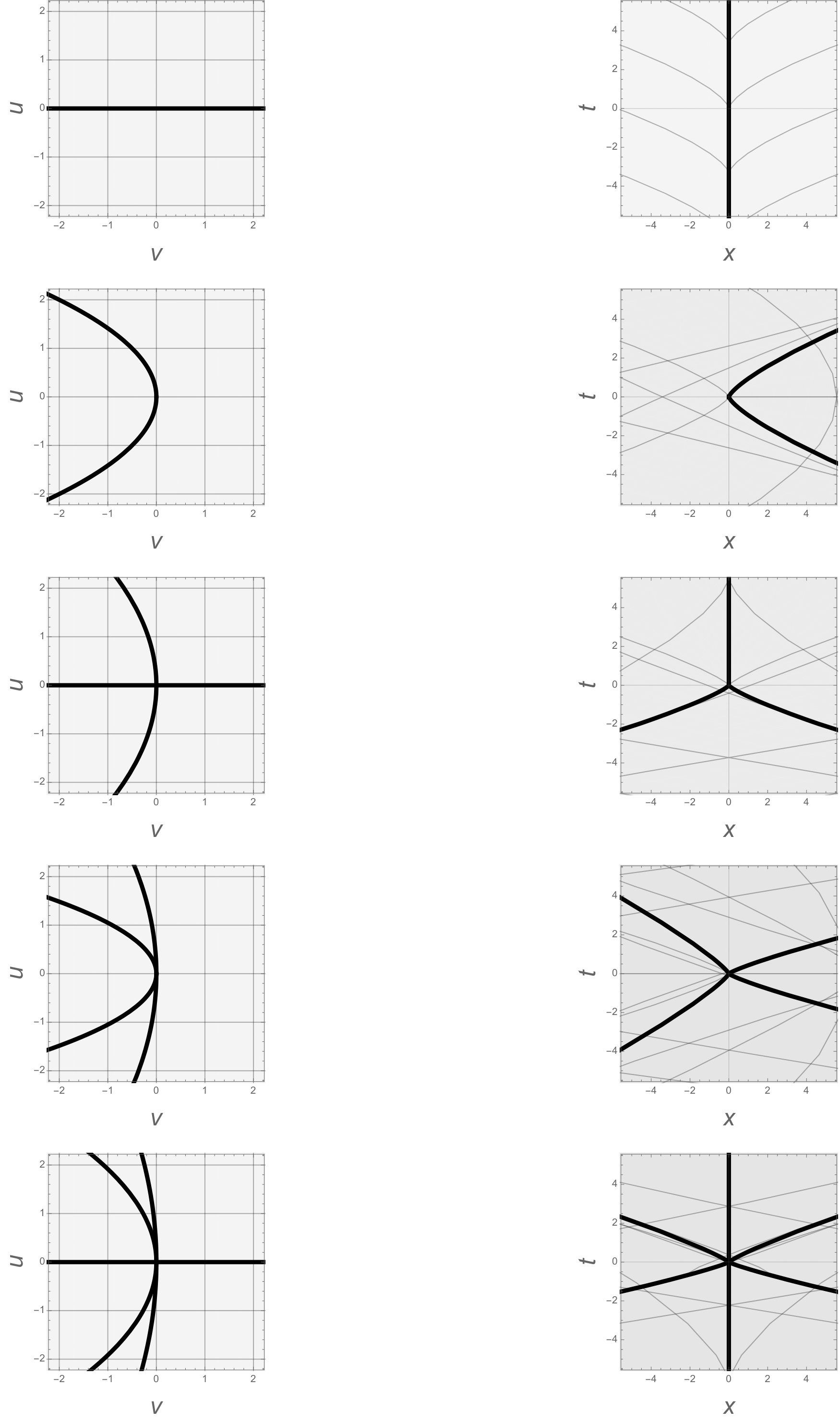 Figure 3
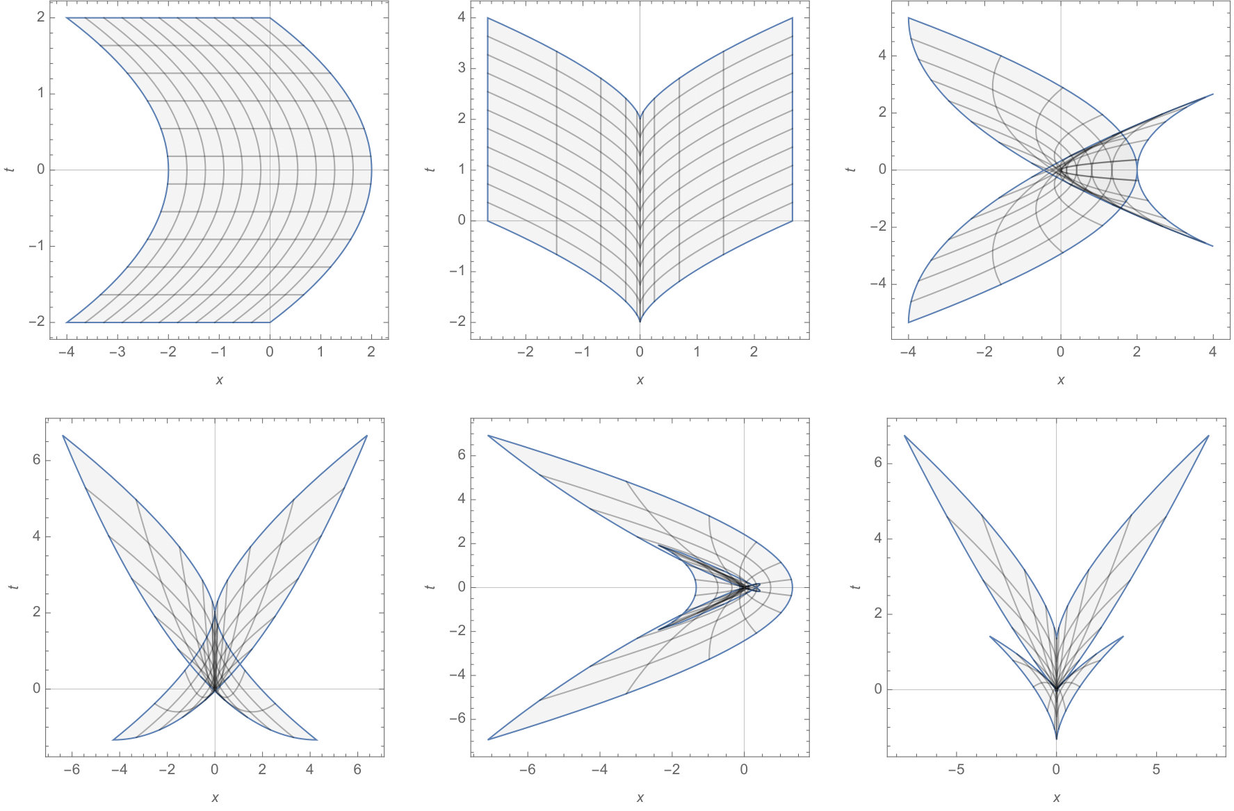 Figure 4
Peer Reviews
No public reviews on file for this paper yet. If you reviewed it on a platform where reviews are public (OpenReview, ICLR, NeurIPS, ICML), you can paste yours below so the community can read it here.
Videos
No videos yet. Explain this paper in a talk, walkthrough, or lecture? Add one.
On the plane into plane mappings of hydrodynamic type. Parabolic case.
B.G. Konopelchenko
Dipartimento di Matematica e Fisica “Ennio de Giorgi”, Università del Salento
and INFN, Sezione di Lecce, 73100 Lecce, Italy
G. Ortenzi
Dipartimento di Matematica Pura ed Applicazioni,
Università di Milano Bicocca, 20125 Milano, Italy
Abstract
Singularities of plane into plane mappings described by parabolic two-component systems of quasi-liner partial differential equations of the first order are studied. Impediments arising in the application of the original Whitney’s approach to such case are discussed. Hierarchy of singularities is analysed by double-scaling expansion method for the simplest -component Jordan system. It is shown that flex is the lowest singularity while higher singularities are given by curves which are of cusp type for , . Regularization of these singularities by deformation of plane into plane mappings into surface to plane is discussed. Applicability of the proposed approach to other parabolic type mappings is noted.
To the memory of B. A. Dubrovin
1 Introduction
Singularities of solutions of hyperbolic and elliptic partial differential equations (PDEs) and associated mappings have been intensively studied during last decades (see e.g. [6, 4, 15, 14, 13, 21, 24, 25, 28, 29, 11, 22, 32, 16, 8, 9, 18, 10] and references therein). Parabolic case, viewed as the degenerate case, has attracted much less attention. It has been addressed essentially only within the study of behavior of solutions of PDEs of mixed type near the transition (sonic) line in fluid- and gas-dynamics (see e.g. [4, 23]) and for heat and diffusion type PDEs of second order [32, 1, 26].
Mappings related to the systems of quasi-linear PDEs of the first order represent particular class of plane into plane mappings. However due to the existence of hodograph transformations (see e.g. [6, 4, 23]) such equations provide us, probably, with the best laboratory for testing the singularity properties of associated mappings and corresponding solutions. Until now such an analysis has been successfully performed for hyperbolic systems (see [15, 14, 13, 21, 24, 25, 28, 29, 11, 22, 32, 16, 8, 9]).
Peculiarity of parabolic regime has been noted in B. Dubrovin fundamental paper on critical behaviour in Hamiltonian PDEs [9], but was not really addressed. Our aim is to fill partially this gap.
In the present paper we will study plane into plane mappings and their singularities governed by the parabolic system
[TABLE]
where is a function of and . System (1) belongs to the class of integrable quasilinear systems of hydrodynamic type [17]. Systems of the type (1) arise also on the transition line for several systems of PDEs of mixed type, for instance, those describing plane motion in gas and fluid dynamics (see e.g. [19, 5]).
Standard hodograph equations for the system (1), i.e. the system
[TABLE]
provides us with the mappings . In the particular case such mappings have simple explicit form
[TABLE]
where function is a solution of the heat equation
[TABLE]
This class of mappings will be studied in detail in the present paper. First, it shown that particular features of the parabolic mappings (3)-(4) and those associated with the system (1) prevent the direct and effective application of the original Whitney approach [35] to them. Some important properties of generic mappings [35] are no more valid for such parabolic mappings. In particular, there are no “excellent” mappings, i.e. those containing only folds and standard cusps [35].
Second, we analyze not only the first order singularities of the mappings (3)-(4), but the whole infinite family of singularities. In contrast to the usually adopted approach to consider the “generic” case (see e.g. [15, 14, 13, 21, 24, 25, 28, 29, 11, 22, 32, 8, 9]) we follow the general principle formulated by Poincaré [27] according to which “one has to study not only a single situation (even generic one) but the whole family of close situations in order to get complete and deep understanding of certain phenomenon”. In our case it means that we have to consider a family of mappings (3) for an infinite family of solutions of the equation (4) which corresponds to family of solutions of the system (2). Higher singularities correspond to the degenerate critical points of higher order for the function obeying (4). So, higher order singularities are unremovable for the family of mappings (3) similar to the degenerate critical points of higher order which are not removable for families of functions (see e.g. [34, 2, 12]).
Using the double scaling expansion technique we show that near the singularity of the order the mapping (3) has locally the form
[TABLE]
where are elementary Schur polynomials of two variables. For the mapping (5) is the flex
[TABLE]
while at it is
[TABLE]
The mappings (5) are singular along the curve . It is shown that this curve is the union of parabolas , for and the union of the line and the parabolas , for , where are roots of Hermite polynomials. Straight lines are images of the line . Images of parabolas are curves which have at origin () -th order singular points with unbounded curvature. For , these curves are cusps.
We discuss also a regularization of singularities of mappings (3)-(4) by deforming them into the mapping of certain surfaces in into the plane . It is shown that -th order singularities of mappings (3)-(4) are regularized by deforming them into mappings -plane.
Applicability of the approach presented in the paper to an analysis of singularities associated with other parabolic systems of PDEs is briefly discussed. Singularities of above -plane mappings, mappings describing symmetries of the system (1) and certain mappings, associated with various integrable parabolic extensions of the system (1) are among them.
In order to emphasize the peculiarity of the parabolic mappings we consider briefly the mappings for hyperbolic two-component systems of hydrodynamic type. It is shown that the Whitney classification approach is an effective one in this case. Higher singularities are also analyzed.
The paper is organized as follows: Section 2 is devoted to the brief recall of the original Whitney’s approach. In section 3 the impediments for application of Whitney’s approach to the mappings governed by the system (1) are discussed. The mappings (3)-(4) and their singularities are studied in section 4. Structure of singular curves for mapping (5) is analyzed in section 5. Regularization of singularities for the mappings (5) is described in section 6. Other parabolic type mappings treatable in the same way are mentioned in section 7. Application of the Whitney’s approach to hyperbolic system is discussed in section 8.
2 Whitney’s theory of singularities
For convenience we briefly recall here some basic facts from the original Whitney’s analysis of singularities of the plane into the plane mappings [35] (see also [2, 31]) with notations adapted to our considerations.
Let be a good -smooth mapping , i.e. such that at every point of the plane either the Jacobian
[TABLE]
is different from zero or at least one of and is different from zero [35]. Singular points of belongs to the curve . Due to the “goodness” condition this curve is smooth and at each point there is nonzero tangent vector . Considering the differentiation along this vector, one introduces the vector field
[TABLE]
which acts on the plane according to the formula
[TABLE]
The point of the singular curve is a fold point if and only if [35]
[TABLE]
and is a cusp point if and only if [35]
[TABLE]
It was shown [35] that near the fold the mapping has a normal form
[TABLE]
while near the cusp it is of the form
[TABLE]
The mapping has been called “excellent” [35] if all its singular points are fold or cusp points. Then the basic theorem A in [35] (p.) states that “arbitrarily near any mapping there is an excellent mapping ”. A crucial condition for this theorem to be valid is that the bad set defined by the three equations (formula (13.5) [35] p.)
[TABLE]
has the defect (codimension) , i.e. the equations (15) are independent. In addition, Whitney has chosen the coordinates systems in the planes and characterized by the conditions
[TABLE]
Such a choice was quite convenient for simplification fo calculations in [35], but, in fact, it is not essential one (see e.g. [31]).
3 Generic parabolic case: impediments
We start with the generic parabolic two-component hydrodynamic type system with two independent variables. It can be reduced to the form [19]
[TABLE]
where is a certain function of and . We will assume that , otherwise the system (17) is totally decoupled.
In the hodograph plane the system (17) is of the form (see e.g. [19])
[TABLE]
This system is compatible iff
[TABLE]
Equations (18) are equivalent to
[TABLE]
Introducing the function such that
[TABLE]
one rewrites the equations (20) as
[TABLE]
where obeys the equation
[TABLE]
Any solution of the equation (23) with given provides us via the relation (22) a solution of the equations (1). On the other hand, for any solution of the equation (23) the formulae (22) define a mapping .
The Jacobian for the mapping (22) is
[TABLE]
and so the mappings (22) are singular along the curve given by
[TABLE]
Note also that the parabolic mappings (22), (23) the correspondence between infinitesimal areas in and planes
[TABLE]
is of the second order near the curve .
At each point of the curve one has a tangent vector
[TABLE]
Following the Whitney’s approach we introduce a vector field
[TABLE]
Its action on images of singular point is given by the formulae
[TABLE]
where and are suitable polynomials in and their and derivatives. On the curve one has the relations
[TABLE]
and so on.
So, for the points on for which one has
[TABLE]
and, consequently, they should be folds according to [35]. If for a point (let us call it [math]) on one has : then, according the first two equation of (29), not only
[TABLE]
but with necessity also
[TABLE]
In this case for . So for the parabolic mappings (22), (23) the equations (32) and (33) are not independent.
This is a crucial difference between the parabolic mappings (22), (23) and generic plane into plane mappings considered in [35]. First for parabolic mappings (22), (23) there are no standard cusp points characterized by condition (12) [35], i.e. by
[TABLE]
Second point is that for parabolic mappings only two of equations (15), i.e.
[TABLE]
characterizing bad set (see [35]) are independent. So the bad set has codimension (defect) and condition for the Theorem 11A in [35] (p.) is not verified. Consequently, the theorem 13A [35] on the existence of excellent mapping near any mapping is not applicable for parabolic mappings (22), (23).
Moreover, for the points on at which and not only
[TABLE]
but also all for . In these points tangent vector for the curve vanishes and vector field is zero too. Such point are no more good points according to [35]. It is noted that these singular points on of higher order are not removable for the family of mappings (22), (23).
Finally we note that Whitney’s choice of coordinate system given by (16) is obviously not admissible for the parabolic mappings described by the equations (18).
These observations clearly indicate that in order to analyze singularities of the mappings (22), (23) one should proceed in a different way.
4 Hierarchy of singularities
Here we present a method to deal with singularities of mappings (22), (23) different from the Whitney’s original one. For convenience we will consider the simplest case with , i.e. the mappings governed by the Jordan system
[TABLE]
In the paper [17] it was shown that this system and its multi-component extensions are integrable, i.e. have infinite family of commuting symmetries. In hodograph plane the system (37) is represented by equations
[TABLE]
and obeys the equation
[TABLE]
The second equation (38) rewritten as implies the existence of a function such that
[TABLE]
Equation (39) means that function obeys the equation (choosing the inessential integration “constant” to be zero). So we have families of mappings given by
[TABLE]
where is any solution of equation
[TABLE]
In the form of equations for critical points of the function above equations has been considered in [17]. It was also shown that differential consequences of (41) and (42) give
[TABLE]
and, hence, and are solutions of the system (37) for any obeying equation (42).
Jacobian for the mappings (41), (42) is
[TABLE]
i.e. (24) with and . So mappings (41), (42) are singular on the curve given by
[TABLE]
Formulas (43) clearly indicates that singularities of the mappings (41), (42) and gradient catastrophes for the system (37) are intimately connected (for other systems see e.g. [6, 4, 15, 14, 28, 29, 11, 22, 32, 8, 9]).
In the case under consideration . So, for the point on at which one has (formula (29))
[TABLE]
So such point should be a fold according to [35].
If at the point on and then (formula (29))
[TABLE]
So such point is not a cusp, according Whitney’s definition (12). Further, if at a point on
[TABLE]
then according to the formulae (29) one has
[TABLE]
These observations clearly show that the vector field is not a right object to establish a gradation of singularities for mappings (41), (42) while the evaluation of the derivatives of with respect to at singular point seems to be a finer tool for that purpose.
So we will use here a standard method of expansion near a point. In our case it is convenient to use particular properties of equations (37)-(39). These equations are obviously invariant under Galilean transformation
[TABLE]
and scaling transformations
[TABLE]
where and are arbitrary parameters. Invariance under Galilean transformations means that for any mapping (41), (42) one can put the point at the origin without loss of generality. Different grading of and for the scaling transformation is preserved for small variations. So for infinitesimal variations and one has
[TABLE]
where is a small parameter. Taking into account all that it is not difficult to show that expansion of function , obeying equation (42), near the origin is of the form
[TABLE]
where and are elementary Schur polynomials (ESP) of two variables defined by the generating relation
[TABLE]
One also has the following expansions
[TABLE]
At the plane the standard multi-scaling expansion near the point is given by (see e.g. [7])
[TABLE]
with parameters and to be determined from the balance of dominant (in ) terms in both parts of the relations (41), i.e.
[TABLE]
and
[TABLE]
At the regular point and, since and , one gets
[TABLE]
So , and at the leading order we have
[TABLE]
This mapping is regular: Jacobian and change of variables , transforms it into
[TABLE]
On singular line (45), , but, in general, . In this case formulae (57), (58) imply that
[TABLE]
So , and
[TABLE]
In variables and it becomes
[TABLE]
and remains singular on the line . Such mapping singularity can be referred as the flex.
If at the point , , i.e. , one has and and mapping near this point is given by
[TABLE]
It is singular on the parabola and the image of this parabola under the mapping (65) is the curve
[TABLE]
These and higher order singularities are characterized by general condition
[TABLE]
In this case one has , and the mappings near such points are (after rescaling and by )
[TABLE]
Thus, the parabolic mappings (41), (42) have hierarchy of singularities which corresponds to the gradation (67) and locally have the form (68). It is noted that the mappings (68) have multiplicity . In the figure 1 we show the image of the mapping (41) near the lowest singular points.
Formulae (52) and (56) imply also that near singular points of order the infinitesimal areas in and planes are proportional to and namely
[TABLE]
So, as
[TABLE]
Double rate decrease of area near singular point is a characteristic feature of parabolic mapping (see also formula (26)).
Finally, it is noted that higher singularities (67), (68) of mappings (41)-(42) are in one-to-one correspondence with higher order gradient catastrophes for the system (37) (cf. [20]).
5 Structure of singular curves
The expansion of near the point characterized by the conditions (67) is given by
[TABLE]
Hence, near the -th order singular point the singular curve (45) has locally the form
[TABLE]
One gets the same result calculating the Jacobian of the mappings (68), namely, .
Due to the properties of ESPs, curves (72) are rather special.
Indeed one has the elementary
Lemma 5.1**.**
Elementary Schur polynomials have the following factorized form
[TABLE]
where are roots of Hermite polynomials.
Proof. Due to the homogeneity of ESP it is obvious that
[TABLE]
Polynomials are defined by the generating relation
[TABLE]
Comparing (75) with the generating relation for the Hermite polynomials [33], i.e.
[TABLE]
one concludes that
[TABLE]
Hence
[TABLE]
Since
[TABLE]
where all roots of are distinct and real ([33]), one has the following factorized form of ESP
[TABLE]
The roots of Hermite polynomials are located symmetrically w.r.t. the origin [33]. Consequently, one gets (73).
Formulae (73) imply that the singular curves (72) for mapping (67) are reducible, namely, they are unions of parabolas for and unions of parabolas and the line for where are roots of Hermite polynomials.
It is easy to see that straight lines
[TABLE]
are images of the line . Images of parabolas are given by curves
[TABLE]
with certain nonzero constants and . The curves (82) have singular points of orders at the origin . The curvature of these curves near the origin is unbounded since
[TABLE]
Tangent-normal pair for the curve (82) behaves smoothly for , while for , it exhibits an instant rotation of angle passing the singular point . The curves (82) are cusps for .
In figure (2) the images of singular curves are shown for .
We would like to note that mappings (68) can be obtained also in a different, formal way. Indeed, let us consider a family of solutions of the equation (42) of the form
[TABLE]
where are free parameters. The mapping (41) for such is given by
[TABLE]
Then the Jacobian and singular curves are defined by the equations
[TABLE]
The equations (67) (for ) imply that
[TABLE]
In such case the mapping (85) takes the form
[TABLE]
while the equation (86) becomes
[TABLE]
So the -th order singular points of the mappings (85) correspond to subspaces of codimension in the space with coordinates .
The mapping (68) and singular curve (72) coincide with the leading order terms in (88) and (89) for small and (, ).
6 Surface into the plane mappings: regularization
In the paper [20] it was shown that the regularization of higher order gradient catastrophes for the system (37) is achieved by embedding it into the multicomponent Jordan system
[TABLE]
Hodograph equations for this system are given by the system [17] (see also [20])
[TABLE]
where function is a solution of the equations
[TABLE]
One can view these relations as the formulae which define mappings of subspace of the hodograph space with coordinate into the plane . Indeed, take a solution of the equations (92). Then, last equations (91)
[TABLE]
define a surface in and the first two equations (91)
[TABLE]
define a mapping -plane. It is noted that both the mapping (94) and the surface are different for different functions . Note also that on the subspace the system (90) and mapping(94) are reduced to the two-component Jordan system (37) and mapping (41). It is readily seen, for instance, for solutions of the system (92) in the form
[TABLE]
where is an arbitrary function.
Mapping (94) is regular at the points where . Indeed, the matrix
[TABLE]
due to the relations (92) and (93) is of the form
[TABLE]
In virtue of (92)-(94) one has
[TABLE]
So, in this case the rank of the matrix is and the mapping (94) is regular (see e.g. [2]).
Let us now compare the mappings (94) and those given by (41),(42). At N=3 a family of functions is formed by solutions of the system
[TABLE]
e.g. in the form (95). Surface for given is defined by the equation
[TABLE]
and the mapping is
[TABLE]
It is regular if on the surface (100)
[TABLE]
The mapping (41), (42) with singularity (, ) is given by
[TABLE]
where is a solution of the equation . It is readily seen that under the restriction to the plane such that the equations (99)-(102) are reduced to those (103). Intersection of the surface with the plane is a singular curve for the mapping (41) and rank of the matrix (97) becomes since . So, a regular mapping is singular under the restriction of to the plane .
This relation viewed in opposite direction provides us with the regularization of the mappings (41), (42). Indeed starting with the mapping (103) for given functions we first enlarge the space to with coordinates . Second we deform the function to a function , satisfying the equations (99) , such that . Such deformation is, for example, the transition in the formula (95) for the same . Then one introduce the surface in given by the equation (100) such that the condition (102) is satisfied and finally one define the mapping -plane given by the formulae (101) . In this deformation the singularity of the mapping (41) becomes a regular point for the mapping .
However, singularities of the mappings (41), (42) for which remain singularities of the mapping (see (98) at ). They can be regularized by extending the preimage plane to with coordinates in the following way. Indeed, first one deforms a given function to a function obeying the equations
[TABLE]
and such that (see (95)). Then one introduces a surface in defined by the equations
[TABLE]
with and consider the mapping given by
[TABLE]
In this case the intersection of the hypersurface defined by the equation with the plane coincides with the singular curve for . Intersection of the hypersurface defined by the second equation (101) gives another curve on the plane . Intersection of these two curves or, equivalently, intersection of the surface defined by both equations (105) with the plane is the singular point of the mapping (41).
The mapping (106) is regular if . So singularity of the mapping (41) (given by (66)) becomes regular point in a deformation of the mapping (41) into mapping .
In order to regularize higher singularities one should increase the dimension . Comparing the formulae (91), (92) and (41)-(42), (57)-(58) and extending the argumentation presented in the above cases, one readily proves the following
Proposition 6.1**.**
The -th order singularity of a mapping (41),(42) with a given function is regularized by deformation of the mapping (41),(42) into the mapping -plane. In this deformation a function is deformed to a function which obeys to the equations
[TABLE]
and satisfies the condition . Surface in is defined by the equations
[TABLE]
and the mapping is given by
[TABLE]
It is noted that such regularization is a local one.
In general an intersection of generic surface in with a plane is empty. However, in our case in virtue of the assumed compatibility of equations (67) a surface defined by (108) intersects the plane at a point which is the -th order singular point of the mapping (41). Namely, the first equation (108), i.e. , defines the hypersurface in intersection of which with the -plane coincides with the singular curve (45) of the mapping (41). Intersection of other hypersurfaces defined by equations (108) at with the plane gives us other curves. All these curves by construction intersect the singular curve at a point of -th order singularity of the mapping (41).
Specifically, for the mappings (68)
[TABLE]
where are ESPs of variables defined by the generating relation
[TABLE]
Then the mapping (109) takes the form
[TABLE]
while the surface is defined by equations
[TABLE]
Intersection of the hypersuperface with the plane is given by the curve which is the singular curve (72). It is easy to show that the system of equations (113) imply that . So the plane is the regularizing surface in this case and the mapping (112) of this plane to the plane is of the form
[TABLE]
i.e.
[TABLE]
First figure 3 (k=1) shows the regularizing surface for the mapping (63). It is the plane and . Second figure 3 (k=2) shows the restriction of the hypersurface defined by the equation to the three-dimensional space with coordinates . Bold line represents the singular curve. Singular point corresponds to on this curve. The plane is the regularizing surface and
At the figure 4 the restrictions of hypersurfaces () and () to the 3-dimensional subspace with coordinates and corresponding singular curves are shown.
Note that the above regularization of the mappings (68) formally can be viewed as the following simple procedure: first, deform the ESPs in (68), namely,
[TABLE]
and then restrict the deformed mapping (68) to the plane .
One can follow similar procedure also in the case when . Namely, first deform
[TABLE]
and then restrict the deformed mapping (68) to the plane . One gets the mappings
[TABLE]
In contrast to the case all the mappings (118) are singular. For instance, for and one has a fold
[TABLE]
and for and one gets
[TABLE]
For mappings (86) the above results give a picture which arises if one considers the contribution of the dominant terms (for small and ) only.
7 On other parabolic type mappings
Approach presented in previous sections can be applied to mappings governed by other parabolic systems of quasilinear PDEs connected with systems (1) and (90).
First, the mappings (91)-(92) are singular if (see (98)). Singular curve lies on the surface given by equations (93) i.e.
[TABLE]
and defined by
[TABLE]
Higher singularities similar to case (39) are characterized by the condition
[TABLE]
At multiscaling expansion near a singular point of the order one has
[TABLE]
Performing this expansion for the mapping (94), one gets
[TABLE]
where and are ESPs with variables .
Since the expansion (124) should be performed on the surface one, using the expansion
[TABLE]
gets from (121) the equations
[TABLE]
So, near to the -th order singular point (123) the mapping (94) have the form (125) and represent themselves the mappings of the surfaces defined by equations (127) into the plane .
At surfaces are given by
[TABLE]
In particular for it is a cylindrical surface generated by the parabola
[TABLE]
and the mapping (125) is
[TABLE]
It is a fold type singularity. In the variables , it assumes the form .
Comparing (66) and (130), one sees that singularity for the mapping (41) is deformed into the fold singularity at and the singular curve at becomes a curve generating surface (129) in
At the surface is a cubic and so on. Thus, -th order singularity (68) at is deformed into the -th order singularity (125) for , while the singular curve (72) is transformed into the surface (128).
For the surface in is given by the equations
[TABLE]
At it is a cylindrical surface defined by equations
[TABLE]
In general, it is readily seen that the -th order singularity (68) becomes the -th order singularity (125) under the deformation while the conditions (67) are transformed into equation (127) defining a surface .
We would like also to note that the singularities (125), (127) are in one-to-one correspondence with the higher order gradient catastrophes fo the system (90) [20].
Second example is connected with the equations which describe higher symmetries of the system (1). They are given by ([17])
[TABLE]
For fixed the hodograph equations are [17]
[TABLE]
which define the mapping for a given obeying the equation .
Further, for the system (90) higher symmetries are described by the system [17]
[TABLE]
where are ESP polynomials of -variables and at . Corresponding hodograph equations [17] define mappings given by
[TABLE]
of surfaces in defined by equations
[TABLE]
where obeys equations (92).
Now, if one consider the family of commuting system (135) , the hodograph equations for their common solutions , instead of (136), (137) assume the form [17]
[TABLE]
where . This system of equation or their more explicit form
[TABLE]
define mappings of of parabolic type.
Finally we note that since the parabolic systems (1), (90), (135) can be viewed as the degeneration of strictly hyperbolic hydrodynamic type systems via certain confluences process [17] the parabolic mappings and their singularities considered in this paper can be recovered via certain degeneration of mappings (confluence type process) and singularities associated with strictly hyperbolic systems of PDES.
8 Hyperbolic case
Singularities of solutions and of mappings for strictly hyperbolic two-component quasilinear systems of PDEs have been studied in several papers (see e.g. [21, 28, 29, 22, 32, 9]). Standard folds and cusps are their generic singularities. Here we will briefly discuss such systems and their singularities in order to emphasize differences between hyperbolic and parabolic cases.
Let us consider the two component system written in terms of Riemann invariants and and characteristic speeds , i.e.
[TABLE]
In hodograph space it is of the form
[TABLE]
and obeys the equation
[TABLE]
The Jacobian of the mapping is
[TABLE]
The mapping is singular if
[TABLE]
or
[TABLE]
First case (144) is realized on the transition line between hyperbolic and elliptic domains. Here we will consider the generic second situation (145), namely, the case
[TABLE]
Let the singular curve be given by . The associated Whitney vector field is
[TABLE]
Calculating , one gets
[TABLE]
If then . So the points where , , are folds according to Whitney’s definition. In the case , , one has
[TABLE]
Thus, at points where , but , , one has
[TABLE]
These points are cusps.
One can show by induction that the gradation of vanishing corresponds to the gradation in derivatives . So it is natural to introduce the gradation of singularities of mapping according to a number of vanishing derivatives of w.r.t. . Namely, we refer to a singularity to be of the order if
[TABLE]
In this case straightforward calculation gives
[TABLE]
and
[TABLE]
So, there is a one-to-one correspondence between the gradation in terms of vector fields and in terms of derivative . At points for which the conditions (152), (153) are verified, the mappings have th order singularities. Such definition of higher order singularities is a natural extension of the original Whitney’s definition of fold and cusps. All the results presented here can be applied in the case , with the exchange . We see that the original Whitney’s approach is fully applicable in the hyperbolic case.
Finally we note that in the weakly-nonlinear case when all the formulae degenerate drastically. Indeed, in this case and, hence, where and are arbitrary functions. Then in the case , it holds
[TABLE]
So this vector fields is factorized and also
[TABLE]
Hyperbolic and elliptic cases will be analysed in more detail in subsequent publication.
Acknowledgments
B.G.K. thanks Prof. W. Schief for useful suggestions on the paper. This research has been supported by grant H2020-MSCA-RISE-2017 Project No. 778010 IPaDEGAN. The author G.O. gratefully acknowledge the auspices of the GNFM Section of INdAM under which part of this work was carried out.
The reference list from the paper itself. Each links out to its DOI / PubMed record.
- 1[1] G. Alessandrini, Critical points of solutions of elliptic equations in two variables, Ann. Scuola Norm. Super. Pisa Cl. Sci. (4) 14 , 229-256 (1987)
- 2[2] V. I. Arnold, S. M. Gusein-Zade and A. N. Varchenko, Singularities of Differentiable Maps vol I-II Basel: Birkh user (1985-1988)
- 3[3] V. I. Arnold, Normal forms of functions in neighborhoods of degenerate critical points, Russ. Math. Surv. 29 10-50 (1974)
- 4[4] L. Bers, Mathematical aspects of subsonic and transonic gas dynamics, John Wiley & Sons, New York (1958)
- 5[5] R. Camassa, G. Falqui and G. Ortenzi, Two-layer interfacial flows beyond the Boussinesq approximation: a Hamiltonian approach, Nonlinearity 30 466-491 (2017)
- 6[6] R. Courant and K.O. Friedrichs, Supersonic Flow and Shock Waves, Springer-Verlag, New York (1962)
- 7[7] P. Di Francesco, P. Ginsparg and J. Zinn-Justin, 2D gravity and random matrices, Physics Reports 254 (1-2) 1-133 (1995)
- 8[8] B. A. Dubrovin, On Hamiltonian Perturbations of Hyperbolic Systems of Conservation Laws, II: Universality of Critical Behaviour, Commun. Math. Phys. 267 117-139 (2006)