On superconvergence of Runge-Kutta convolution quadrature for the wave equation
Jens Markus Melenk, Alexander Rieder

TL;DR
This paper analyzes the convergence properties of Runge-Kutta convolution quadrature methods for wave equation scattering problems, demonstrating improved convergence rates and providing new estimates on Dirichlet-to-Impedance maps.
Contribution
It introduces a novel estimate on the Dirichlet-to-Impedance map that enhances understanding of superconvergence in Runge-Kutta convolution quadrature for wave equations.
Findings
Higher convergence rate for the derivative-based Runge-Kutta method.
Numerical results confirm the sharpness of the theoretical analysis.
New estimate reduces frequency dependence in Helmholtz problem maps.
Abstract
The semidiscretization of a sound soft scattering problem modelled by the wave equation is analyzed. The spatial treatment is done by integral equation methods. Two temporal discretizations based on Runge-Kutta convolution quadrature are compared: one relies on the incoming wave as input data and the other one is based on its temporal derivative. The convergence rate of the latter is shown to be higher than previously established in the literature. Numerical results indicate sharpness of the analysis. The proof hinges on a novel estimate on the Dirichlet-to-Impedance map for certain Helmholtz problems. Namely, the frequency dependence can be lowered by one power of (up to a logarithmic term for polygonal domains) compared to the Dirichlet-to-Neumann map.
Click any figure to enlarge with its caption.
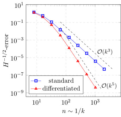 Figure 1
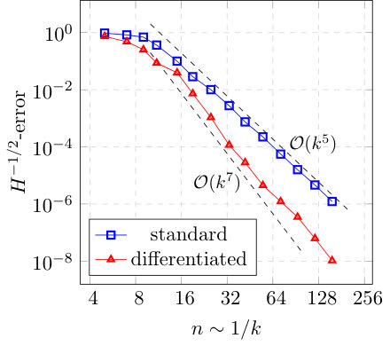 Figure 2
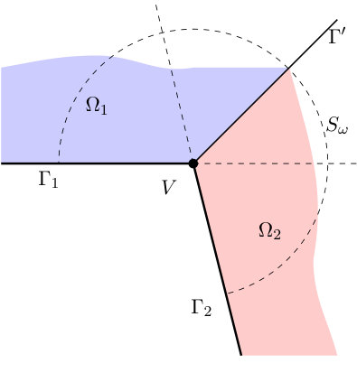 Figure 3
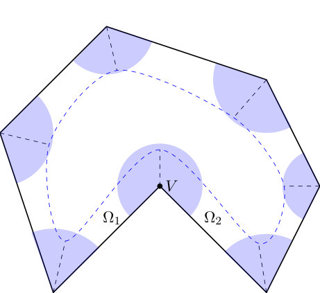 Figure 4
Peer Reviews
No public reviews on file for this paper yet. If you reviewed it on a platform where reviews are public (OpenReview, ICLR, NeurIPS, ICML), you can paste yours below so the community can read it here.
Videos
No videos yet. Explain this paper in a talk, walkthrough, or lecture? Add one.
On superconvergence of Runge-Kutta convolution quadrature for the wave equation
Jens Markus Melenk
Alexander Rieder
Abstract
The semidiscretization of a sound soft scattering problem modelled by the wave equation is analyzed. The spatial treatment is done by integral equation methods. Two temporal discretizations based on Runge-Kutta convolution quadrature are compared: one relies on the incoming wave as input data and the other one is based on its temporal derivative. The convergence rate of the latter is shown to be higher than previously established in the literature. Numerical results indicate sharpness of the analysis. The proof hinges on a novel estimate on the Dirichlet-to-Impedance map for certain Helmholtz problems. Namely, the frequency dependence can be lowered by one power of (up to a logarithmic term for polygonal domains) compared to the Dirichlet-to-Neumann map.
1 Introduction
Boundary element methods have established themselves as one of the standard methods when dealing with scattering problems, especially if the domain of interest is unbounded. First introduced for stationary problems, beginning with the seminal works [BH86a, BH86b] these methods have steadily been extended to time-dependent problems; see [Say16] for an overview. The method of convolution quadrature (CQ), introduced by Lubich in [Lub88a, Lub88b], is a convenient way of extending the stationary results to a time-dependent setting.
It is well-known that the convergence rate of a Runge-Kutta convolution quadrature (RK-CQ) as introduced in [LO93], is determined by bounds on the convolution symbol in the Laplace domain. Namely, a bound of the form
[TABLE]
leads to convergence rate , as was proven in [BLM11], see also [BL11, LO93] for earlier results in this direction. Thus one might expect that changing the symbol to would increase the convergence order by one.
When considering discretizations of the wave equation using boundary integral methods, this is not always the case. Instead, it has been observed that sometimes a “superconvergence phenomenon” appears, where the observed convergence rate surpasses those predicted, see [RSM20a, RSM20b, Rie17].
In this paper, we give a first explanation why such a phenomenon occurs in the model problem of sound soft scattering, i.e., the discretization of the Dirichlet-to-Neumann map. We expect that similar phenomena can also explain the improved convergence rate for the Neumann problem or more complex scattering problems. The proof relies on the observation that the -weighted Dirichlet-to-Neumann map can be decomposed into a Dirichlet-to-Impedance map plus the identity operator. For the Dirichlet-to-Impedance operator, it was observed in [Ban14] that an improved bound holds compared to the Dirichlet-to-Neumann map as long as the geometry is given by the sphere or the half-space. It is then conjectured that a similar bound holds for smooth, convex geometries. In this paper, provided that we restrict the Laplace parameter to a sector, we generalize this result to a much broader class of geometries, namely, smooth or polygonal geometries, without convexity assumption. This will then immediately give the stated improved bound for the convolution quadrature scattering problem. In the case of polygons, the result holds in a slightly weaker form in that it contains an additional logarithmic term.
As a consequence of this observation, it may often be beneficial to select a problem formulation with an extra time derivative. In many situations, such formulations are even the natural choice, see, e.g., [BR18, BL18, BLS15], and especially when one works with the wave equation as a first order system as in [RSM20b].
Another way of looking at this phenomenon is that when using a standard formulation (i.e., taking as in Proposition 3.2 without using a time derivative on the data), then the discrete integral will exhibit a superconvergence effect.
We point out that the present paper focuses on a semidiscretization of the problem with respect to the time variable. For practical purposes one would also have to take into account the discretization in space using boundary elements. We also mention that while popular, CQ is only one possibility to apply boundary integral techniques to wave propagation problems. Notably also space-time based methods have gained popularity [GNS17, GMO*+*18, JR17] in recent years.
2 Model Problem and Notation
We consider a sound soft scattering problem for acoustic waves. For a bounded Lipschitz domain with , the problem reads: Find such that
[TABLE]
Here is a given incoming wave, i.e., also solves the wave equation, and we assume that for it has not reached the scatterer yet. The problem can be recast by decomposing the total wave into the incoming and outgoing wave, , where solves:
[TABLE]
This will be the problem we are discretizing.
For simplicity, we consider two possible cases. The bounded Lipschitz domain has either a smooth boundary or is a polygon. While we expect that the results and techniques can be generalized to the case of piecewise smooth geometries, such an extension would lead to a much higher level of technicality in the present paper. Although we focus on the exterior scattering problem as our motivating model problem all of the main results also hold for the interior Dirichlet problem.
We end the section by fixing some notation. We write for the usual (complex valued) Sobolev spaces on or . On the interface we also need fractional spaces for , see, e.g., [McL00, AF03] for precise definitions. We also set . We write for the exterior and interior trace operator, and for the normal derivative. We note that in both cases, we take the normal to point out of the bounded domain . We write {\left\llbracket\gamma u\right\rrbracket}:=\gamma^{+}u-\gamma^{-}u and for the trace jump and mean, and {\left\llbracket\partial_{n}u\right\rrbracket}:=\partial_{n}^{+}u-\partial_{n}^{-}u for the jump of the normal derivative.
The notation abbreviates with implied constants independent of critical parameters, in particular the parameter that appears throughout this work. For (relatively) open sets we introduce the scalar product .
2.1 Boundary Integral Methods and Convolution Quadrature
It is well-known that scattering problems of the form presented in Section 2 can be solved by employing boundary integral methods, see [Say16] for a detailed time domain treatment. For the frequency domain, results can be found in most textbooks on the subject, see [SS11, Ste08, McL00, GS18, HW08].
The use of boundary integral methods for discretizing the time domain scattering problem dates back to the works [BH86a, BH86b], where also important Laplace domain estimates of the form (3.2) were first shown.
For s\in\mathbb{C}_{+}:=\big{\{}z\in\mathbb{C}:\,\operatorname{Re}(z)>0\big{\}}, we introduce the single and double layer potentials
[TABLE]
where is the fundamental solution for the operator :
[TABLE]
Here denotes the first kind Hankel function of order zero, see [McL00, Chap. 9]. Finally, we introduce the boundary integral operators induced by the potentials:
[TABLE]
In practice, these operators can be realized explicitly as integrals over the boundary since for sufficiently smooth functions , the following equations hold:
[TABLE]
The operator we consider for discretizing (2.1) is the Dirichlet-to-Neumann map.
Definition 2.1**.**
For , given , let solve
[TABLE]
We then define the operators
[TABLE]
In practice, the following well-known proposition gives an explicit way to calculate .
Proposition 2.2** (see, e.g., [LS09, Appendix 2]).**
The Dirichlet-to-Neumann map can be written as
[TABLE]
RK-CQ was introduced by Lubich and Ostermann in [LO93]. It provides a simple and general way of approximating convolution integrals by a high order method and has the great advantage that only the Laplace transform of the convolution symbol is required. We only very briefly introduce the method and notation.
Let be a holomorphic function in the half plane . Let denote the Laplace transform and its inverse. We (formally) introduce the operational calculus by defining
[TABLE]
where is such that the inverse Laplace transform exists and the expression above is well defined.
For a Runge-Kutta method given by the Butcher tableau , , the convolution quadrature approximation of with time step size is given, for any function with for , by the expression
[TABLE]
where the matrix valued function is given by
[TABLE]
The extension to operator valued functions is straight forward. In practice, we only consider evaluating at the discrete time steps .
We make the following assumptions on the Runge-Kutta method, slightly stronger than [BLM11].
Assumption 2.3**.**
- (i)
The Runge-Kutta method is A-stable with (classical) order and stage order . 2. (ii)
The stability function satisfies for . 3. (iii)
The Runge-Kutta coefficient matrix is invertible. 4. (iv)
The method is stiffly accurate, i.e., .
Remark 2.4**.**
*Assumption 2.3 is satisfied by the Radau IIA and Lobatto IIIC methods, see [HW10]. Also note that the order conditions imply that for such methods. *
Our analysis will employ the following result on RK-CQ using Laplace domain estimates:
Proposition 2.5** ([BLM11, Thm. 3]).**
Assume that is holomorphic in the half plane and that there exist such that satisfies the following bounds for all :
[TABLE]
Assume that the Runge-Kutta method satisfies Assumption 2.3. Let r>\max\big{(}p+\mu_{1},p,q+1\big{)} and satisfy . Then there exists such that for ,
[TABLE]
The constant C depends on , , , the constants , , and the Runge-Kutta method.
3 Main results
To simplify the notation, we introduce a symbol for the sectors in Proposition 2.5. Throughout this work we fix and and set
[TABLE]
Remark 3.1**.**
*The choice of and in the definition of is arbitrary, and all our estimates will hold for any choice, although all the constants will depend on and . *
We are now able to state the main result of the paper. We start by stating the standard convergence result for discretizing the Dirichlet-to-Neumann map.
Proposition 3.2** (Standard method).**
Let for some and . Let be the exact normal derivative and denote the standard CQ-approximation. Then there exist constants and such that the following estimate holds for and :
[TABLE]
with a constant depending on the terminal time , the Runge-Kutta method, , and .
Proof.
Follows from the well-known bound
[TABLE]
(see for example[LS09]) and Proposition 2.5. ∎
We will observe numerically in Section 5 that Proposition 3.2 is essentially sharp. Thus, when considering the differentiated equation, one expects an increase in order by one, which follows directly from Proposition 2.5. But for the Dirichlet-to-Neumann map the increase of order is even greater, as long as one assumes slightly higher regularity of the data.
Theorem 3.3** (Method based on differentiated data).**
Let . Let g\in C^{r}\big{(}[0,T],H^{1}(\Gamma)\big{)} satisfy . Let be the exact normal derivative and denote the CQ-approximation using as input data. Then, for all , there exist constants and such that the following estimate holds for and :
[TABLE]
The constant depends on , the terminal time , the Runge-Kutta method, , and . If is smooth, one can take .
Proof.
We apply Proposition 2.5. By linearity, we can write the Dirichlet-to-Neummann operator as
[TABLE]
The second operator (in frequency domain) is independent of . It is a simple calculation that in such cases, i.e., if for all , the convolution weights satisfy . Thus, we have
[TABLE]
Since stiff accuracy implies and , the operator is reproduced exactly by the CQ. A similar decomposition was already invoked in [BLM11] to explain a superconvergence phenomenon for a scalar problem. Combining standard estimates, e.g., [LS09, Table 1], with Theorem 3.4 shows that the Dirichlet-to-Impedance map satisfies
[TABLE]
By Proposition 2.5 and by estimating the logarithmic term by for arbitrary , we obtain (3.3). ∎
While Theorem 3.3 is the main motivation for this paper, its proof is based on another result, which may be of independent interest.
Theorem 3.4**.**
Let . Let be a bounded smooth Lipschitz domain. The following estimate holds for the Dirichlet-to-Neumann map:
[TABLE]
If is a bounded Lipschitz polygon, then one has
[TABLE]
The constant depends only on and the parameters , defining the sector .
Proof.
Due to its lengthy and technical nature, we defer the proof to Section 4. For smooth geometries it is shown as Corollary 4.11. Polygonal domains are handled in Corollary 4.19. ∎
Remark 3.5**.**
*The regularity requirement is stronger than the expected requirement . This is due to the construction of the boundary layer function (see (4.15)). *
Since all our results hold for both the interior and exterior problem, we can also easily treat the case of an indirect BEM formulation.
Corollary 3.6** (Indirect formulation).**
Let and assume that is smooth. Then, the operator satisfies the bound
[TABLE]
Let for some with . Let be the exact density and be its CQ-approximation.
Then there exist constants and such that the following estimate holds for and :
[TABLE]
The constant depends on , the Runge-Kutta method, , and .
If is a polygon, then
[TABLE]
and
[TABLE]
where is arbitrary, and depends additionally on .
Proof.
We can write . Thus the statements follows from Theorems 3.3 and 3.4. ∎
4 Proofs
The proof of Theorem 3.4 hinges on three main observations, which require some technical work to be made rigorous:
In 1d on , the interior Dirichlet-to-Neumann map is given by . 2. 2.
The existing -estimate’s poor dependence is mainly caused by boundary layers. 3. 3.
Boundary layers are essentially a 1d phenomenon, so observation 1 applies.
4.1 Preliminaries
There are many ways of defining fractional order Sobolev spaces. A convenient way of working with them is by introducing them via the real method of interpolation. Given Banach spaces with continuous embedding and parameters , , we define the interpolation norm and space as follows:
[TABLE]
When working with the Helmholtz equation, it is convenient to work with -weighted norms:
Definition 4.1**.**
For an open (or relatively open) set , parameters and , we define the weighted Sobolev norms
[TABLE]
For , the corresponding norms are defined via interpolation. If we want to include boundary conditions, we write for the interpolation space between and , but equipped with the weighted norms (4.2).
The dual norms are defined by
[TABLE]
For the most part we will be working with the closed surface . There, the norms and coincide. By Lemma A.1 we also have for and bounded domains the norm equivalence
[TABLE]
with implied constants independent of .
We start with some well-known -explicit estimates for the (modified) Helmholtz equation.
Lemma 4.2** (Well posedness).**
Let . The sesquilinear form
[TABLE]
associated to is elliptic in the sense that, using , it satisfies
[TABLE]
Proof.
We calculate:
[TABLE]
Since in the sector this concludes the proof. ∎
Lemma 4.3** (Trace estimates).**
For and , let satisfy
[TABLE]
Then the following estimates hold for the traces of :
[TABLE]
Proof.
We start with the normal derivative. For any and any with we calculate:
[TABLE]
where in the last step we select as the minimal energy function, satisfying
[TABLE]
By [Say16, Prop. 2.5.1], admits the estimate and (4.4) follows.
For the Dirichlet trace, we get using the multiplicative trace estimate and the same lifting :
[TABLE]
The estimate for the impedance trace then follows trivially. ∎
The previous lemma shows that for a priori estimates in terms of standard Sobolev norms the constants involved have some dependence. The next lemmas show that the use of the weighted norms introduced in Definition 4.1 avoids such dependencies:
Lemma 4.4**.**
The operators satisfy the bounds:
[TABLE]
Proof.
The multiplicative trace estimate and Young’s inequality give
[TABLE]
Combining this with the standard trace estimate concludes the proof in view of (4.3). ∎
Lemma 4.5** (Dirichlet problem).**
Let , . For any there exists a unique solution to the problem
[TABLE]
The function satisfies the a priori bound
[TABLE]
The implied constant depends only on and the constants , characterizing .
Proof.
Existence follows using the usual theory of elliptic problems. For the a priori bound, we first note that by [MS11, Lemma 4.22], there exists a lifting satisfying
[TABLE]
Thus the remainder solves:
[TABLE]
As the sesquilinear form from Lemma 4.2 is elliptic, we get with defined there
[TABLE]
Lemma 4.6** (Neumann problem).**
Let . Then for every there exists a unique solution to the problem
[TABLE]
* satisfies the a priori bound*
[TABLE]
The implied constant depends only on and on , characterizing .
Proof.
Follows easily from the weak formulation and (4.8). ∎
We also have the following trace inequality in a weighted -norm:
Lemma 4.7**.**
If we can estimate:
[TABLE]
Proof.
Follows easily from the weak definition of , the Cauchy-Schwarz inequality, and (4.8). ∎
4.2 Smooth geometries
In order to prove a first version of Theorem 3.4, we consider a simplified setting of smooth geometry and Dirichlet trace. Closely following the ideas from [MS99, Mel02], we construct a lowest order boundary layer function that will be the basis for all further estimates.
Lemma 4.8** (Boundary fitted coordinates).**
Let be a smooth local parametrization of . Define as
[TABLE]
where is the outer normal vector to at the point .
For sufficiently small, is a smooth diffeomorphism onto F\big{(}\mathcal{O}\times(-\varepsilon,\varepsilon)\big{)}. It holds that and . Additionally, satisfies
[TABLE]
where and are smooth and is invertible.
Proof.
We only show (4.12). We select a smooth orthogonal basis of the tangent space at , denoted by . This implies that Q:=\big{(}e_{1}(\widehat{x}),\dots,e_{d-1}(\widehat{x}),n(\widehat{x})\big{)} is orthogonal.
[TABLE]
Here , and thus . We further compute:
[TABLE]
where collects the remaining terms. For sufficiently small , depending only on and , we can linearize the inverse in (4.13) to get (4.12) with \widetilde{T}:=\big{(}\widetilde{T}_{1}\widetilde{T}_{1}^{T}\big{)}^{-1} (the latter inverse exists since and thus also has full rank). ∎
Lemma 4.9**.**
Assume that has a smooth boundary . For any and for every solving
[TABLE]
together with there exists a function with the following properties:
- (i)
, 2. (ii)
, 3. (iii)
* with*
[TABLE]
The implied constant depends only on and , characterizing . 4. (iv)
For define the set . Then, the following estimates hold for all with constants independent of :
[TABLE] 5. (v)
The analogous statement also holds for the exterior problem , replacing by in (ii).
Proof.
We only show the case of the interior problem and abbreviate . We work in boundary fitted coordinates as described in Lemma 4.8. First assume, that , i.e., is supported by the part of the boundary parametrized by . The change of variables formula shows that if solves , then solves:
[TABLE]
with and (see, e.g., [Eva98, Step 7 of proof of Thm. 4, Sec. 6.3.2]). On the other hand, if satisfies
[TABLE]
then solves
[TABLE]
We set and define with the function
[TABLE]
in the boundary fitted coordinates. By (4.12), we have . Differentiating out we obtain for some smooth functions , , , , and
[TABLE]
where, in the last step, we exploited the definition of . From its definition, one can easily see that satisfies the estimates
[TABLE]
Transforming back gives (4.14) for the part of parametrized by . Assertion (iv) follows easily from the definition, as the exponential decay dominates all powers of . This allows us to smoothly cut off for large and extend it by [math] to the whole domain. For general , we use a smooth partition of unity to decompose into functions with local support. ∎
As the next step, we lower the regularity requirement on .
Corollary 4.10**.**
Let have a smooth boundary . For any and for every with solving
[TABLE]
there exists a function with the following properties:
- (i)
. 2. (ii)
\left\|\partial_{n}^{-}(u-u_{BL})-s\big{(}\gamma^{-}u-\gamma^{-}u_{BL}\big{)}\right\|_{H^{-1/2}(\Gamma)}\lesssim\left\|\gamma^{-}u\right\|_{H^{1}(\Gamma)}.** 3. (iii)
* The implied constant depends only on and the constants , characterizing .* 4. (iv)
For introduce . Then, the following estimates hold for all with constants independent of :
[TABLE] 5. (v)
The analogous statement also holds in the case of the exterior problem upon replacing by in (i) and (ii).
Proof.
In order to apply Lemma 4.9, we need -regularity of . We fix a function with the following properties:
[TABLE]
This can be either seen by realizing as the interpolation space between and and using [BS78, Lemma] or constructed directly via the usual mollifiers as done in [AF03, Thm. 2.29]: The approximation estimate follows from [AF03, Eqn (20)] and an interpolation argument. See also [AF03, Sec. 7.48] for how to trade Sobolev regularity for approximation properties of the mollified function.
Let denote the solution to
[TABLE]
Since , we can apply Lemma 4.9 to construct . Assertion (i) then follows by construction. For (iii): we note that by Lemmas 4.5 and 4.9:
[TABLE]
For (ii), we use Lemma 4.3 and (4.9) to get that
[TABLE]
Similarly, we have
[TABLE]
Assertion (iv) follows directly from Lemma 4.9 (iv) and (4.16). ∎
Corollary 4.11**.**
Let be smooth and . Let and solve
[TABLE]
Then
[TABLE]
The analogous statement holds for the exterior problem upon replacing by in (4.17).
Proof.
Follows by writing . The impedance trace of vanishes by Corollary 4.10 (i). The impedance trace of the remainder is uniformly bounded with respect to via Corollary 4.10 (ii). ∎
4.3 Polygons
In this section, we consider a polygonal domain as an example of a non-smooth domain. In order to match the boundary layer solutions from Lemma 4.9 at corners, we solve an appropriate transmission problem, similarly to what was done in [Mel02]. We refer to Figure 1(b) for the geometric situation.
We first need one additional Sobolev space. For a smooth curve and , we introduce
[TABLE]
where denotes the distance to the endpoints of .
4.3.1 A transmission problem in a cone
In this section, we investigate certain transmission problems. These will allow us to match different boundary layer functions in the vicinity of a corner of the domain. We start by investigating the special case of a transmission problem on a sector or an infinite cone. Due to its special structure, we can derive sharper estimates for the normal derivative than what can be obtained from the energy methods used in Lemma 4.16 below.
We introduce some notation. Given , we define the infinite cone
[TABLE]
with opening angle and by removing from its bisector:
[TABLE]
Next, we define the sector , which is just the truncated cone . For its boundary, we write \Gamma_{\pm\omega}:=\big{\{}(r\cos(\pm\omega),r\sin(\pm\omega)),\;r\in(0,1)\big{\}} for the two parts of the boundary of the sector that are adjacent to the origin and set . Finally, we need to define the normal jump across interfaces. If denotes a smooth interface separating domains and we define the normal jump across via
[TABLE]
where the normal vectors are taken to point out of respectively.
Lemma 4.12**.**
Consider the solution to the following problem on the infinite cone for and with :
[TABLE]
Then, the following statements hold for :
- (i)
For each there exist constants , such that for all
[TABLE] 2. (ii)
There exists a constant such that satisfies the estimates
[TABLE]
The constants depend only on the opening angle , the parameter , and the choices of and in the definition of .
Proof.
We first show (ii) in Steps 1–3 and then (i) in Step 4.
Step 1: We start with an energy estimate in exponentially weighted spaces, namely, for any the following estimate holds:
[TABLE]
with a constant only depending on , , , and .
We fix some notation. We write , and analogously for . Also we set for the transmission data. The proof follows [Mel02, Prop. 6.4.6] verbatim. The sesquilinear form satisfies an inf-sup condition: There is depending only on such that
[TABLE]
This can be seen by taking, for given in the infimum, the function in the supremum and performing elementary calculations. Next, we show that . This follows also verbatim [Mel02, Prop. 6.4.6] using [Mel02, Lemma A.1.8]. Specifically, by [Mel02, Lemma A.1.8] it suffices to ascertain that for we have
[TABLE]
We conclude that the solution satisfies for some constant depending only on the choice of .
Step 2: For a ball of radius around any point with we can apply standard elliptic regularity (interior regularity, regularity for homogeneous Dirichlet conditions, and regularity for transmission problems—see, e.g., [Mel02, Lemmas 5.5.5, 5.5.7, 5.5.8]) to get
[TABLE]
A Besicovich covering argument (see, e.g., [Mel02, Lemma 4.2.14] for details) by such balls and local trace estimates show that for
[TABLE]
where the implied constant depends only on , , and , .
Step 3: We show that . Fix a cut-off function with on and . We consider the following lifting of the jump using a single layer potential for the Laplacian:
[TABLE]
Since , we have by the mapping properties of the single layer potential (see [CWGLS12, Thm. 2.17]) that with
[TABLE]
for some depending on and . The jump relations of the single layer operator provide (see, e.g., [McL00, Thm. 6.11]) and on . Since and , and we see that is the -function solving
[TABLE]
Since the right-hand side and the Dirichlet boundary conditions are in , standard elliptic regularity theory (see, e.g., [McL00, Thm. 4.24]) shows .
Step 4 (proof of (i)): The 2D Sobolev embedding theorem and (4.23) show the desired estimate for . The argument leading to (4.23) can be iterated and thus yields the stated estimates for any fixed .
Step 5: Inspection of the proof reveals that all constants (if at all) depend continuously on . Since we are only interested in in a compact set determined by the constants from the definition of we can make all the constants independent of . ∎
Having studied the transmission problem in a dimensionless form in Lemma 4.12, we can transfer the results to the setting we actually require using a scaling argument.
Lemma 4.13**.**
Fix . For and , let solve the transmission problem on the sector :
[TABLE]
Recall that denotes the parts of adjacent to the origin. Then
[TABLE]
The constants depend only on , the parameter , and the choices of and in the definition of .
Proof.
We denote by the circular arc that is part of . Write with . Let be the function solving
[TABLE]
that is given by Lemma 4.12. Then we define . Lemma 4.12 and a simple scaling argument gives the following estimates for (for any ):
[TABLE]
The remainder then solves
[TABLE]
We note that for this Dirichlet problem with piecewise smooth data that are exponentially small in , Lemma 4.5 gives , which is exponentially small in . Applying [McL00, Thm 4.24] then gives, since vanishes on :
[TABLE]
which is again exponentially small in . The estimate (4.26) follows. ∎
We need the following modification of [MPW17, Lemma 3.13].
Proposition 4.14**.**
Let be a Lipschitz domain. Define the Besov space (cf. (4.1))
[TABLE]
For and every , there exists a function with
[TABLE]
The constant depends only on the domain .
Proof.
This is essentially [MPW17, Lemma 3.13]. The only modification needed is that we consider the -norm on the right-hand side instead of the -norm, which is the reason for getting penalized by a factor instead of a factor as in [MPW17, Lemma 3.13]. The result follows from the same proof, only noting that one can bound using the Cauchy-Schwarz inequality
[TABLE]
and the last factor produces a factor . ∎
Lemma 4.15**.**
Let solve (4.25). Then, there exists a constant depending only on , and the parameters in the definition of such that
[TABLE]
Proof.
For , select as in Proposition 4.14 with to be chosen later. We calculate for , i.e., the two parts of adjacent to the origin:
[TABLE]
Since is a one-dimensional line segment, we can use the Sobolev embedding [Tar07, Sec. 32] to estimate
[TABLE]
Overall, we get using the properties of from Proposition 4.14 and the estimates on from (4.24):
[TABLE]
Choosing completes the proof. ∎
We are now in a position to study a more general transmission problem, namely, allowing for Dirichlet jumps and more general Neumann transmission data.
Lemma 4.16** (Transmission problem).**
Let be an open Lipschitz domain. Let be a smooth interface that splits into two disjoint Lipschitz domains and .
Given , , there exists a unique solution to the following problem:
[TABLE]
Additionally, the following estimate holds:
[TABLE]
If and are polygons, is a straight line, and can be decomposed as
[TABLE]
for some , , and , then exists pointwise almost everywhere and
[TABLE]
Proof.
Proof of (4.27): Since is assumed in , we can extend it by [math] to a function such that (see for example [McL00, Thm. 3.33])
[TABLE]
We solve a Dirichlet problem on with data to obtain and extend it by [math] to . Then we solve the following problem on : Find such that
[TABLE]
where denotes the trace operator on . The function then solves the transmission problem. The estimate (4.27) follows from Lemmas 4.5 to bound and, in order to bound , the ellipticity of the sesquilinear form (see Lemma 4.2) together with the trace estimate (Lemma 4.4) to estimate the contribution .
Proof of (4.16) for : Introduce \mathcal{V}:=\partial\Gamma^{\prime}\cup\{\text{vertices of \Omega}\}. Since and are piecewise smooth and on and the right-hand side is homogeneous, the solution is smooth up to the boundary with the exception of the vertices of and near the interface . Hence, exists pointwise everywhere on . To show the estimate (4.16), we consider test functions v\in V:=\{v\in C^{\infty}(\overline{\mathcal{O}})\,|\,v\text{ vanishes in a neighborhood of \mathcal{V}}\}. Since exists pointwise on and vanishes in a neighborhood of , the duality pairing is well-defined and an integration by parts gives
[TABLE]
Since is dense in (because consists of finitely many points), the equation (4.29) actually holds for all . Given we select with as the lifting given by (4.7) in Lemma 4.3, which satisfies . This implies
[TABLE]
By the trace theorem we have . Taking the supremum over all yields (4.16) for the case .
Proof of (4.16) for : If , we lift this contribution separately by solving the corresponding transmission problem (4.25). The estimate follows by applying Lemma 4.15 and a suitable localization. ∎
4.3.2 Corner layers
Before we can bound the functions used to match boundary layers, we must control the jump between two boundary layer solutions. We start with a very simple geometric situation.
Lemma 4.17**.**
Fix . Consider the sector and let . Consider the two Cartesian coordinate systems and , each given by one of the straight sides of the sector and such that the components and of the bisector are positive. In polar coordinates (with , ) these coordinates are given by
[TABLE]
For define
[TABLE]
- (i)
On the line segment the following estimates hold with
[TABLE] 2. (ii)
The normal jump across can be decomposed as
[TABLE]
where the orientation of the normal is arbitrarily fixed and is independent of . 3. (iii)
There holds .
Proof.
We work in polar coordinates, which are related to the coordinates and by (4.30). For brevity of notation we introduce the constants , and note .
Proof of (i): We start with the estimate for the Dirichlet jump and calculate on :
[TABLE]
We estimate:
[TABLE]
An analogous computation gives:
[TABLE]
Next we compute the tangential derivative of {\left\llbracket\gamma u\right\rrbracket} on :
[TABLE]
The first term is handled analogously to the -term. For the second term we use the crude estimate and get:
[TABLE]
Interpolating (4.32) and (4.33) then gives (4.31).
Proof of (ii): In polar coordinates, the normal derivative on of a function is (up to the sign) given by . Thus it is sufficient to estimate the angular derivatives.
On , we calculate for the angular derivative:
[TABLE]
After substracting the contribution from the second term, the two terms are structurally similar to the derivative of {\left\llbracket\gamma u\right\rrbracket}. Hence, we analogously get for h_{2}:={\left\llbracket\partial_{n}u\right\rrbracket}-h_{1}sg(0)e^{-s\mu c_{2}r}:
[TABLE]
To control we calculate for :
[TABLE]
Proof of (iii): We identify with the interval . A direct calculation shows . A test function can be represented as . Hence, an integration by parts yields
[TABLE]
Thus, . Furthermore, we have . Interpolation then yields . ∎
4.3.3 Decomposing the DtN-operator
In Section 4.2 we discussed the DtN-operator for smooth geometries. Here, we study the case of polygonal domains. We will do so by introducing corner layers, similarly to what was done in [Mel02, Sec. 7.4.3].
The following Theorem 4.18 presents a decomposition of the DtN-Operator into several contributions. To describe them, we need some notation as illustrated in Fig. 1(b). The polygon has vertices and edge connects with (we set and and, for simplicity of notation, we assume that consists of a single component of connectedness). is the bisector of the angle at vertex . The subdomains are confined by four curves: , the bisectors at and (dashed black in Figure 1(a)), and a fourth curve completely contained in and sufficiently close to (dashed blue in Figure 1(a)) . We set and, for convenience . We fix with and near . Finally, for each vertex we let be a cut-off function with for such that on .
Theorem 4.18**.**
Let be a polygon, . Let with . Let solve
[TABLE]
Then can be decomposed as such that for a depending only on :
- (i)
* and for each . Additionally, .* 2. (ii)
For each the function is in for each and . Furthermore, on and exists on each edge , , and
[TABLE]
Furthermore, . 3. (iii)
The remainder satisfies
[TABLE]
The analogous statement holds for the exterior problem upon replacing by in (i)-(iii).
Proof.
1. step (construction of ): For each , let be the boundary fitted coordinates obtained by an affine parametrization of the line that contains by and denoting by the (signed) distance from that line. Write for the function on in the coordinates and extend it and -stable to the line. We define, in boundary fitted coordinates , the function . That is, the function is given by applying the construction from Lemma 4.9. We have by construction on and .
2. step (construction of ): The function is discontinuous across the bisectors . The corner layers corrects this. Focussing on the bisector , let and be the edges meeting at . Fix such that on . On the sector define as the solution of the following transmission problem:
[TABLE]
Up to translation and rotation, we are essentially in the setting of Lemmas 4.16 and 4.17. That is, on and the function has the form given in Lemma 4.17 so that (taking additionally the effect of into account) we arrive at
[TABLE]
where . For the normal derivative, Lemma 4.17 provides the representation {\left\llbracket\partial_{n}(\chi_{BL}u_{BL})\right\rrbracket}(x)=h_{1}sg(0)e^{-s\mu\left|x\right|}+h_{2}(x) with
[TABLE]
By Lemma 4.16, we therefore get
[TABLE]
Furthermore, Lemma 4.16 provides for on the bound
[TABLE]
Noting that on , the asserting of (ii) follows.
3. Step (Construction of ): The function is defined as . It satisfies the equation with satisfying
[TABLE]
The bounds of Lemma 4.3 and 4.5 then conclude the proof.
4. Step (exterior domains): The result for the exterior problem follows along the same lines. ∎
From Theorem 4.18 we deduce the following result for the DtN operator under slightly lower regularity requirements:
Corollary 4.19**.**
Let b a polygon and . Let and solve
[TABLE]
Then
[TABLE]
The analogous statement holds for the exterior problem upon replacing by .
Proof.
We employ the smoothing technique as in Corollary 4.10: By smoothing, on a length scale or by interpolation, one can construct a function such that for each edge and such that
[TABLE]
This can be done in two steps: first, one defines the approximation edgewise and in a second step ensure continuity at the vertices of by introducing an appropriate correction, e.g., by a piecewise linear function. The remainder of the proof is then as in Corollary 4.10. ∎
5 Numerical Examples
In this section, we compare the performance of the numerical schemes of Theorem 3.3 with the more standard method of Proposition 3.2 for an interior scattering problem. That is, we compare the Runge-Kutta convolution quadrature approximation by the following two methods:
, which is denoted “standard method”, and
, which is denoted “differentiated method”.
We use two different Runge-Kutta methods of the Radau IIA family, one with 3 and one with 5 stages. For the 3-stage version, we have and . We therefore expect a convergence rate of order for the standard method and full classical order up to logarithmic terms for the differentiated scheme.
In order to show that our theoretical estimates are sharp, we also look at the 5-stage method. There, the stage order is and the classical order . The expected rates are therefore and respectively for the two numerical schemes up to logarithmic terms.
For simplicity, we consider the interior scattering problem and prescribe an exact solution as the travelling wave
[TABLE]
The wave direction is selected as , and the other parameters were and . We integrated until the end time . In order to show that the method works with the predicted rates, even for non-convex geometries, we consider the classical L-shaped geometry, given by the vertices
[TABLE]
As the space discretization, we employ a Galerkin boundary element method of order , based on a code developed by F.-J. Sayas and his group at the University of Delaware. A sufficiently refined grid is employed to be able to focus on the temporal error. Instead of evaluating the -error, we compute the quantity
[TABLE]
Here denotes the -orthogonal projection onto the BEM space. Since the grid is sufficiently fine and fixed, this should not impact the observed convergence rates. The operator was taken because it gives an (-independent) equivalent norm on .
In Figure 5.1, we observe that the rates from Proposition 3.2 and Theorem 3.3 are obtained as predicted. We conclude that while the fact that the rate jumps by order , even though the modification of the scheme is of order one, is at first surprising, this can be rigorously explained by Theorem 3.3. Observations of this type provided the main motivation for the investigations in this work.
Acknowledgments: The authors gratefully acknowledge financial support by the Austrian Science Fund (FWF) through the research program “Taming complexity in partial differential systems” (grant SFB F65).
Appendix A Norm equivalence of interpolation spaces
Lemma A.1**.**
Let be a bounded domain. For and let be defined as in Definition 4.1. Define
[TABLE]
Then there are constants , depending only on and such that for all
[TABLE]
Proof.
We use [KMR20, Lemma 4.1] with and there. As given there, we set as well as , where we omitted the argument for brevity. In [KMR20, Lemma 4.1] the interpolation norm based on and the interpolation seminorm based on . We note that .
1. step: We claim . This claim follows from the following two estimates using the Poincaré inequality:
[TABLE]
Conversely,
[TABLE]
2. step: The norm equivalence (A.1) follows from [KMR20, Lemma 4.1]. ∎
The reference list from the paper itself. Each links out to its DOI / PubMed record.
- 1[AF 03] R. A. Adams and J. J. F. Fournier. Sobolev spaces , volume 140 of Pure and Applied Mathematics (Amsterdam) . Elsevier/Academic Press, Amsterdam, second edition, 2003.
- 2[Ban 14] L. Banjai. Time-domain Dirichlet-to-Neumann map and its discretization. IMA J. Numer. Anal. , 34(3):1136–1155, 2014.
- 3[BH 86a] A. Bamberger and T. Ha Duong. Formulation variationelle espace-temps pour le calcul par potentiel retardé d’une onde acoustique. Math. Meth. Appl. Sci. , 8:405–435, 1986.
- 4[BH 86b] A. Bamberger and T. Ha Duong. Formulation variationnelle pour le calcul de la diffraction d’une onde acoustique par une surface rigide. Math. Methods Appl. Sci. , 8(4):598–608, 1986.
- 5[BL 11] L. Banjai and C. Lubich. An error analysis of Runge-Kutta convolution quadrature. BIT , 51(3):483–496, 2011.
- 6[BL 18] L. Banjai and C. Lubich. Runge–Kutta convolution coercivity and its use for time-dependent boundary integral equations. IMA J. Numer. Anal. , 06 2018.
- 7[BLM 11] L. Banjai, C. Lubich, and J. M. Melenk. Runge-Kutta convolution quadrature for operators arising in wave propagation. Numer. Math. , 119(1):1–20, 2011.
- 8[BLS 15] L. Banjai, C. Lubich, and F.-J. Sayas. Stable numerical coupling of exterior and interior problems for the wave equation. Numer. Math. , 129(4):611–646, 2015.