Getting the Most Out of Your VNFs: Flexible Assignment of Service Priorities in 5G
Francesco Malandrino, Carla-Fabiana Chiasserini

TL;DR
This paper introduces FlexShare, a flexible and efficient method for sharing VNFs in 5G networks by dynamically assigning service priorities, leading to cost savings and improved performance.
Contribution
It proposes a novel approach to VNF sharing that dynamically adjusts service priorities across VNFs, enhancing resource efficiency and cost-effectiveness.
Findings
FlexShare outperforms baseline solutions in real-world scenarios.
Dynamic priority assignment improves resource utilization.
The methodology operates in polynomial time for practical deployment.
Abstract
Through their computational and forwarding capabilities, 5G networks can support multiple vertical services. Such services may include several common virtual (network) functions (VNFs), which could be shared to increase resource efficiency. In this paper, we focus on the seldom studied VNF-sharing problem, and decide (i) whether sharing a VNF instance is possible/beneficial or not, (ii) how to scale virtual machines hosting the VNFs to share, and (iii) the priorities of the different services sharing the same VNF. These decisions are made with the aim to minimize the mobile operator's costs while meeting the verticals' performance requirements. Importantly, we show that the aforementioned priorities should not be determined a priori on a per-service basis, rather they should change across VNFs since such additional flexibility allows for more efficient solutions. We then present an…
Click any figure to enlarge with its caption.
 Figure 1
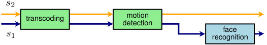 Figure 2
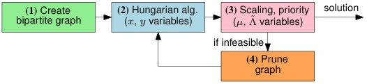 Figure 3
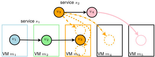 Figure 4
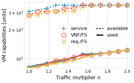 Figure 5
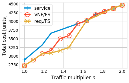 Figure 6
 Figure 7
 Figure 8
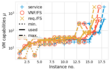 Figure 9
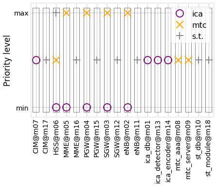 Figure 10
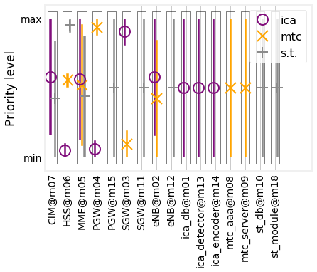 Figure 11
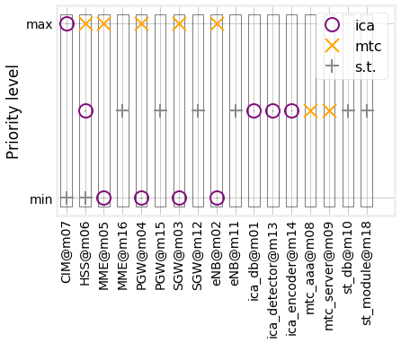 Figure 12
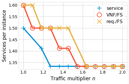 Figure 13
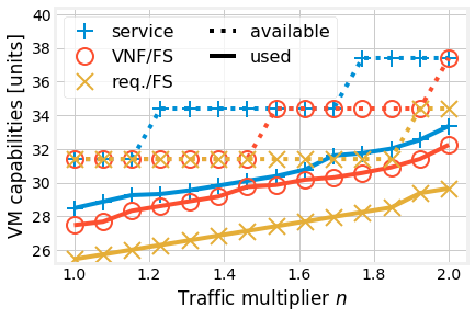 Figure 14
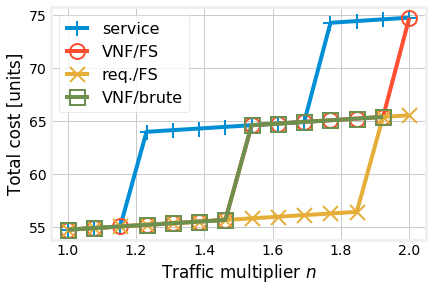 Figure 15
 Figure 16
 Figure 17
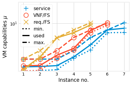 Figure 18
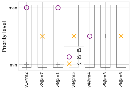 Figure 19
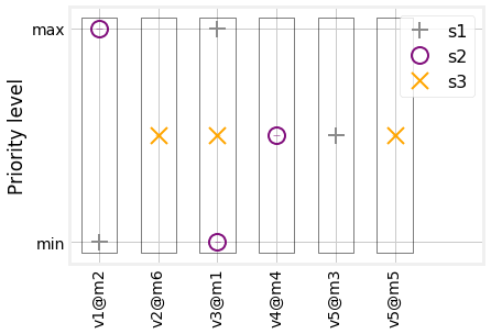 Figure 20
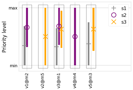 Figure 21
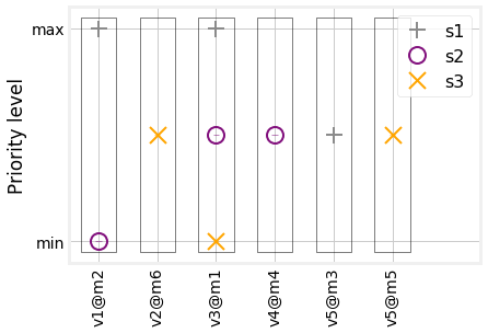 Figure 22
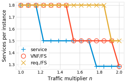 Figure 23
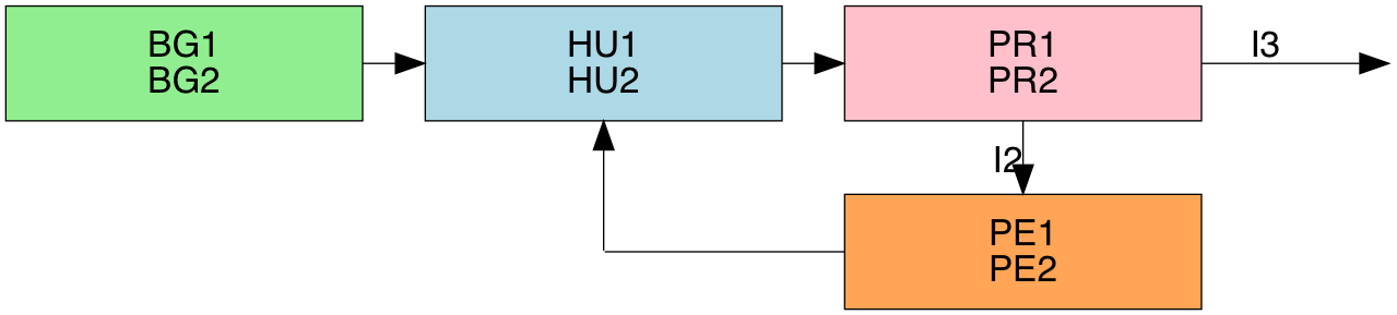 Figure 24
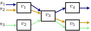 Figure 25
| Symbol | Type | Meaning |
| Parameter | Maximum capability to which VM can be scaled up | |
| Parameter | Target delay for service | |
| Parameter | Jitter applied when assigning per-request priorities | |
| Parameter | Computational capability needed to process one request at VNF | |
| Set | Set of VMs | |
| Random var. | Describes the priority assigned to requests of service upon entering VNF | |
| Parameter | Per-VNF priority of service at VNF | |
| Aux. var. | Sojourn time of requests of service at VNF | |
| Set | Set of services | |
| Set | Set of VNFs | |
| Binary var. | Whether requests of service use the instance of VNF running at VM | |
| Binary var. | Whether VM runs VNF | |
| Parameter | Fixed cost incurred when activating VM | |
| Parameter | Proportional cost incurred when using one unit of computational capability for VM | |
| Aux. var. | Arrival rate at VNF of requests that are given priority over requests of service | |
| Real var.† | Arrival rate at VNF of requests that are given priority over requests of service | |
| Parameter | Rate at which requests of service enter VNF | |
| Real var. | Computational capability to use for VM |
| VNF | Rate | Requirement |
| Intersection collision avoidance (ICA) | ||
| eNB | 117.69 | |
| EPC PGW | 117.69 | |
| EPC SGW | 117.69 | |
| EPC HSS | 11.77 | |
| EPC MME | 11.77 | |
| Car information management (CIM) | 117.69 | |
| Collision detector | 117.69 | |
| Car manufacturer database | 117.69 | |
| Alarm generator | 11.77 | |
| See through (CT) | ||
| eNB | 179.82 | |
| EPC PGW | 179.82 | |
| EPC SGW | 179.82 | |
| EPC HSS | 17.98 | |
| EPC MME | 17.98 | |
| Car information management (CIM) | 179.82 | |
| CT server | 179.82 | 5 |
| CT database | 17.98 | |
| Sensing (IoT) | ||
| eNB | 50 | |
| EPC PGW | 50 | |
| EPC SGW | 50 | |
| EPC HSS | 5 | |
| EPC MME | 5 | |
| IoT authentication | 20 | |
| IoT application server | 20 | |
Peer Reviews
No public reviews on file for this paper yet. If you reviewed it on a platform where reviews are public (OpenReview, ICLR, NeurIPS, ICML), you can paste yours below so the community can read it here.
Videos
No videos yet. Explain this paper in a talk, walkthrough, or lecture? Add one.
Getting the Most Out of Your VNFs:
Flexible Assignment of Service Priorities in 5G
Francesco Malandrino*∗,†, Carla-Fabiana Chiasserini†,∗*
: CNR-IEIIT, Torino, Italy : Politecnico di Torino, Torino, Italy
Abstract
Through their computational and forwarding capabilities, 5G networks can support multiple vertical services. Such services may include several common virtual (network) functions (VNFs), which could be shared to increase resource efficiency. In this paper, we focus on the seldom studied VNF-sharing problem, and decide (i) whether sharing a VNF instance is possible/beneficial or not, (ii) how to scale virtual machines hosting the VNFs to share, and (iii) the priorities of the different services sharing the same VNF. These decisions are made with the aim to minimize the mobile operator’s costs while meeting the verticals’ performance requirements. Importantly, we show that the aforementioned priorities should not be determined a priori on a per-service basis, rather they should change across VNFs since such additional flexibility allows for more efficient solutions. We then present an effective methodology called FlexShare, enabling near-optimal VNF-sharing decisions in polynomial time. Our performance evaluation, using real-world VNF graphs, confirms the effectiveness of our approach, which consistently outperforms baseline solutions using per-service priorities.
I Introduction
5G networks differ from their previous counterparts in several key features. Among them, two especially relevant aspects are the computational capabilities with which networks are endowed, and the relationship between network operators and vertical industries (e.g., multimedia content providers, automotive industries, smart factories).
Thanks to software-defined networking (SDN) and network function virtualization (NFV), cellular networks have now the ability to process data, as well as to forward them. A set of hosts, be them physical servers or virtual machines, run virtual network functions (VNFs), performing network-related (e.g., firewalls), or service-specific (e.g., video transcoding) tasks. Such an arrangement is beneficial for both mobile network operators (MNOs), who can fully utilize their infrastructure, and verticals, who can use it to deploy their services and enjoy lower delays.
The relationship between MNOs and verticals is evolving accordingly. Verticals can enter business relations with MNOs, using their network infrastructure to provide services with the required quality-of-service level. Indeed, vertical services are specified as a set of interconnected VNFs, along with per-service target key performance indicators (KPIs), e.g., throughput, delay, or reliability. Supporting services of multiple verticals, with different target KPIs, through the same MNO infrastructure, is possible thanks to network slicing. This is a powerful concept enabling multiple logical networks as independent business operations, on a common physical infrastructure [1]. Notably, network slicing also accounts for composed services, i.e., service VNF graphs including sub-graphs, each representing a child service [2]. Indeed, different network slices may contain one or more common sub-slices [3, 4], a typical example being the evolved packet core (EPC) of cellular networks [2].
When creating a network slice, the MNO is in charge of assigning to it the needed resources (e.g., virtual machines and links connecting them), and of deciding which VNFs each host should run. This problem, known as VNF placement, pursues the twofold objectives of (i) ensuring that the target KPIs are met, and (ii) minimizing the cost for the MNO. Importantly, the latter can be achieved by sharing individual VNFs or sub-slices, among multiple services whenever possible.
The vast majority of studies on VNF placement [5, 6, 7] implicitly assume that (i) all placement decisions are made by one entity, typically the NFV Orchestrator (NFVO) of the Management and Network Orchestration (MANO) framework [8, 4], and (ii) such entity makes fine-grained decisions about how individual hosts and links are used. However, such a behavior is not the only one included in standards, and is not typical of real-world 5G implementations. Indeed, ETSI IFA 007 specifies four possible granularity levels for placement decisions, namely, Point of Presence (PoP) – e.g., a data center –, zone111Zone refers to a subset of hosts within a PoP. group, zone, and individual host, with real-world 5G implementation efforts envisioning the NFVO to make PoP-level decisions [9, 10].
Fine-grained decisions on sharing VNF instances within individual PoPs are made by other, non-MANO entities, as envisioned by IETF [4, Sec. 3], the NGMN alliance [11, Sec. 8.9], and 5G-PPP [3, Sec. 2.2.2]. For sake of concreteness, we take as a reference the latter architecture, which includes an entity called Software-Defined Mobile Network Coordinator (SDM-X). As summarized in Fig. 1, the SDM-X works at a lower abstraction level than the MANO entities, and is in charge of solving the VNF-sharing problem, managing the VNFs that are common to multiple services.
This is the problem that, differently from traditional VNF placement studies, we address in this paper. Specifically, we solve the VNF-sharing problem within a PoP, by deciding, for each newly requested service,
- •
whether it is possible and convenient to re-use the existing VNF instances222For simplicity, and without loss of generality, we will refer to common VNFs only, instead of common VNFs and sub-slices.;
- •
which priority to give to services sharing the same VNF, in order to meet the target KPIs;
- •
whether and to which extent to scale up the computational capability of virtual machines (VMs) within the PoP.
A simple instance of the VNF-sharing problem we address is presented in Fig. 2. For each VNF of the newly-requested service , we have to decide which VM shall run it (this decision is trivial for , for which no instance exists yet) and the priority to assign to requests, e.g., REST queries, of each service in each shared VNF.
Contributions. To effectively tackle the VNF-sharing problem, we make the following main contributions:
- •
we observe that allowing flexible priorities for each VNF and service, makes it possible to meet KPI targets at a lower cost for the MNO;
- •
based on the above key observation, we present a system model capturing all the relevant aspects of the VNF-sharing problem and the entities it involves, including the capacity-scaling and priority-setting decisions it requires;
- •
leveraging convex optimization, we devise an efficient, integrated solution methodology called FlexShare, able to make swift, high-quality decisions concerning VM usage, priority assignment, and capability scaling;
- •
we evaluate the computational complexity of FlexShare and study its performance against real-world VNF graphs.
In the rest of the paper, we begin by presenting an example motivating the need for flexible priorities across VNFs (Sec. II). Then, Sec. III introduces our system model and problem formulation, while Sec. IV describes the FlexShare solution strategy. Our reference scenarios and numerical results are discussed in Sec. V. Finally, after reviewing related work in Sec. VI, Sec. VII concludes the paper.
II The role of priorities
Before addressing the problem of whether it is convenient to share a VNF among multiple services or not, let us highlight the role of priorities while sharing a VNF instance. Three main approaches can be adopted for VNF sharing:
- •
per-service priority, associated with each service and constant across different VNFs;
- •
per-VNF priority, associated with each service and VNF, thus, given a service, it may vary across different VNFs;
- •
per-request priority, associated with individual service requests, e.g., REST queries, it may vary across the different VNFs on a per-request basis.
In the following example, we focus on the first two steps of the above flexibility ladder and show how higher flexibility in priority assignment is associated with a higher efficiency in handling service traffic.
Example 1** (The importance of flexible priorities).**
Consider the two services, and , depicted in Fig. 3, requested by a vertical specialized in video surveillance systems. includes two VNFs executing transcoding and motion detection, respectively, while is composed of and a VNF performing face recognition. Each VNF should run in its own VM, and network transfer times between VMs are neglected. Adopting a well-established and convenient approach [6, 7], let us model VNFs as M/M/1 traffic queues processing service requests, and the services as queuing chains, with arrival rates 2\text{,}\mathrm{r}\mathrm{e}\mathrm{q}\mathrm{u}\mathrm{e}\mathrm{s}\mathrm{t}\mathrm{s}\mathrm{/}\mathrm{m}\mathrm{s} and $\lambda_{2}=$1\text{\,}\mathrm{r}\mathrm{e}\mathrm{q}\mathrm{u}\mathrm{e}\mathrm{s}\mathrm{t}\mathrm{s}\mathrm{/}\mathrm{m}\mathrm{s}, respectively. Also, consider service delay as the main performance metric and let the target average delay be 1.1\text{,}\mathrm{ms} for both services. Then assume that, given the allocated computation resources, the service rate of the transcoding and motion detection is $\mu_{\text{tc}}=\mu_{\text{md}}=\mu=$5\text{\,}\mathrm{r}\mathrm{e}\mathrm{q}\mathrm{u}\mathrm{e}\mathrm{s}\mathrm{t}\mathrm{s}\mathrm{/}\mathrm{m}\mathrm{s}, while that of face recognition is 9.15\text{,}\mathrm{r}\mathrm{e}\mathrm{q}\mathrm{u}\mathrm{e}\mathrm{s}\mathrm{t}\mathrm{s}\mathrm{/}\mathrm{m}\mathrm{s}$$.
To meet the delay targets, requests must traverse the transcoding and motion detection with a combined sojourn time of , while requests must do the same in at most (i.e., the target average delay minus the sojourn time at the face recognition VNF of 0.14\text{,}\mathrm{ms}$$). We now show that there is no way of setting per-service priorities that allow this.
Case 1: Higher priority to .* This choice would make intuitive sense since requests have to go through more processing stages than requests, within the same deadline. In this case, requests incur a sojourn time of 0.33\text{,}\mathrm{ms}* for each of the common VNFs, resulting in a total delay *$D_{1}=$0.8\text{\,}\mathrm{ms}, well within the target. However, the sojourn time of requests at each of the shared VNFs becomes [12, Sec. 3.2]: 0.83\text{,}\mathrm{ms}$$, which results in a total delay of 1.66\text{,}\mathrm{ms}.*
Case 2: Higher priority to .* It is easy to verify that giving higher priority to implies that misses its target delay.*
Case 3: Equal priority.* Giving the same priority to both services results in a sojourn time of 0.5\text{,}\mathrm{ms}$$ for each of the common VNFs, and in a total delay of 1\text{,}\mathrm{ms} and 1\text{,}\mathrm{ms}0.14\text{,}\mathrm{ms}.*
Flexible priorities.* Assume that and have priority in the transcoding and in the motion detection VNF, respectively. Then, 1.095\text{,}\mathrm{ms}, and 1.08\text{,}\mathrm{ms}.*
In conclusion, the above example shows that no combination of per-service priorities results in both and meeting their target delays. Instead moving one step up the flexibility ladder, i.e., assigning different priorities to service traffic flows across VNFs, allows the MNO to meet the vertical’s requirements while increasing efficiency in resource usage, hence lowering the costs. As we will see later, even better performance can be obtained through per-request priorities.
III System model and problem formulation
As mentioned earlier, the SDM-X has to use the VMs under its control to provide the newly-requested services with the required KPIs and at the minimum cost. Specifically, it has to make decisions on (i) whether existing VNF instances should to be shared; (ii) if so, how to assign the priorities to different services sharing the same VNF instance; (iii) scaling up the computational capabilities of the VMs if needed and possible.
As these decisions are made with reference to a single PoP, processing times are the dominant contribution with respect to network latency, and we therefore neglect the latter. This assumption is also justified by the ongoing work in the datacenter networking community (see, e.g., [13]), where (i) switching is highly optimized, hence network delays tend to be very small, and (ii) network topologies tend to be highly regular, hence network delays between any two VMs tend to be very similar across pairs of VMs. It follows that network delays are often, within a single PoP, often negligible with respect to processing times.
Next, Sec. III-A describes how all the entities that are involved in the VNF-sharing problem can be described, while Sec. III-B defines the problem objective and constraints.
III-A System model
The system model includes VMs , and VNFs 333VNFs can, in general, include multiple virtual deployment units (VDUs); without loss of generality, we consider that each VNF includes only one VDU. Also, we assume that no VNF requires isolation.. Each VM runs (at most) one VNF, modeled as an M/M/1 queue with FIFO queuing and preemption, as widely assumed in recent works [6, 7, 14]. Also, let be the maximum computation capability to which VM can be scaled up. We underline that, although in this work we focus on computational capability, memory and storage could be easily accommodated as well. We refer to a VM as active if it hosts a VNF, and we express through binary variables whether VM runs VNF .
Different VNFs have different computational requirements, which are modeled through parameter , expressing how many units of computational capability are needed to process one request in one second. A VNF with requirement running on a VM with capability takes time unit to process a service request. Using the same VM for a VNF with requirement yields a processing time of time units. Notice how values do not depend on the service using VNF .
Services include one or more VNFs, and service requests arrive at VNF with rate ; VNFs that are not used by a certain service have -values equal to [math]. Through the parameters, we can account for arbitrarily complex service (VNF) graphs where the number of requests can change between VNFs, and some requests may visit the same VNF more than once. We focus on the maximum average delay of service as target KPI, although our model can be seamlessly extended to account for different (or additional) KPIs, e.g., service request drop probability.
Each VM uses a quantity of computational capability, which can be scaled up till . Then the rate at which a VNF deployed at VM processes service requests results to be . Finally, binary variables express whether service uses the instance of VNF at VM ; this allows us to account for the fact that multiple instances of the same VNF can be deployed at different VMs. For clarity, the above parameters and variables are summarized in Tab. I.
III-B Problem formulation
We now discuss the objective of the VNF-sharing problem and the constraints we need to honor.
Objective. The high-level goal of the MNO is to minimize the cost, which consists of two components: a fixed cost paid if VM is activated, and a proportional cost paid for each unit of computational capability used therein. The objective is then given by:
[TABLE]
Capability and instance limits. We must account for the maximum value to which the capability of each VM can be scaled up:
[TABLE]
Also, we can have at most one VNF per VM:
[TABLE]
and only active VMs can be used, i.e.,
[TABLE]
Service times. Each service has a maximum average service time that must be honored. Since, as discussed earlier, processing time is the dominant component of service time, this is equivalent to imposing:
[TABLE]
where is the sojourn time (i.e., the time spent waiting or being served) experienced by requests of service at VNF . By convention, we set if service does not include VNF .
As detailed below, sojourn times, in turn, depend on:
- •
the computational capability requested by the VNFs;
- •
the service request arrival rate at the VNFs ;
- •
the priority of the service requests at the traversed VNFs;
- •
the computational capability assigned to the VM hosting the VNF instance processing the requests.
Using [12, Sec. 3.2] and [15], we can generalize the expression used in Example 1 and write the sojourn time of requests of service at VNF , as:
[TABLE]
where is the VM hosting the instance of VNF used by service , i.e., .
In (6), represents the arrival rate of requests (of any service) arriving at VNF that are given a priority higher than a generic request of service . Let be the random variable describing the priority assigned to requests of service at VNF , then we have:
[TABLE]
The intuitive meaning of (7) is that grows as it becomes more likely that requests of other services are given higher priority over requests of service .
Problem complexity. The actual expression of depends on the type of the variables and is not guaranteed to be linear, convex, or even continuous. It follows that, in the general case, the problem of setting the priorities in such a way to optimize (1) has NP-hard complexity and is thus impractical for realistically-sized problem instances. Indeed, as will be more clear from Sec. III-B1 and Sec. III-B2, finding the optimum in the per-request priority case, would require to search over all possible distributions of .
Below, we compute for the relevant cases of per-VNF priorities and uniformly-distributed, per-request priorities.
III-B1 Per-VNF priorities
We recall that, if per-VNF priorities are supported as in Sec. II, then all requests of each service entering VNF are given the same, deterministic priority. It follows that, denoted such a priority with , in the per-VNF case is always distributed according to a Dirac delta function centered in , i.e., . Hence, is discontinuous and given by:
[TABLE]
where is the Heaviside step function. Indeed, intuitively a request of service will be queued after all requests of services with higher priority than (since if ), after half of the requests of services with the same priority as (since if ), and before all other requests (since if ).
III-B2 Per-request priorities
This case corresponds to higher flexibility and implies that priorities could follow any distribution. Below, we focus on the simple, yet relevant, case where priorities are distributed uniformly between and . In this case, let us define the quantity , whose value can be computed through the convolution of the pdfs of and . Following the steps in [16], we get:
[TABLE]
Once the are known, the values can be computed by replacing (9) in (7), obtaining:
[TABLE]
In this case, it is also possible to prove that the choice of parameter has no impact on the solution space, hence, on the decisions that are made.
IV The FlexShare solution strategy
In light of the problem complexity, we propose a fast, yet highly effective, solution strategy, named FlexShare, which runs iteratively and consists of four main steps, as outlined in Fig. 4. The first step, detailed in Sec. IV-A, consists in building a bipartite graph including the VNFs to deploy, and the VMs that are active or can be activated. The edges of the graph express the possibility of using a VM to provide a VNF, either by sharing an existing instance or by deploying a new one. Edges are labeled with the cost associated with each decision, i.e., the and/or terms contributing to the objective (1). In step 2, the Hungarian algorithm [17] is run on the generated bipartite graph, yielding the optimal, minimum-cost assignment of VNFs to VMs, i.e., the - and -variables of the problem.
Given these decisions, step 3 aims at assigning the priorities and finding the amount of computational capability to use in every VM. To this end, a simpler (namely, convex) variant of the problem defined in Sec. III-B is formulated and solved, as detailed in Sec. IV-B.
If step 3 results in an infeasible problem, we prune the bipartite graph (step 4). The underlying intuition is that a cause for infeasibility is overly aggressive sharing of existing VNF instances. Therefore, as detailed in Sec. IV-C, edges that result in an overload of VMs are removed from the bipartite graph. After pruning, the algorithm starts a new iteration with step 2. Moving from one iteration to the next means reducing the likelihood that VNF instances are shared between services, and thus increasing the cost incurred by the MNO, due to the fixed cost terms. The procedure stops as soon as one feasible solution is found.
IV-A Steps 1–2: Bipartite graph and Hungarian algorithm
The bipartite graph. The purpose of the bipartite graph is to represent (i) the possible VNF assignment decisions, i.e., which VNFs can be provided at which VMs and which VNFs can be shared among services, and (ii) the associated cost incurred by the MNO.
More formally, the bipartite graph is created according to the following rules:
a vertex is created for each VNF and for each VM; 2. 2.
an edge is drawn from every VNF to every unused VM; 3. 3.
an edge is drawn from every VNF to every VM currently running the same VNF, provided that the maximum computational capability of the VM is sufficient to guarantee stability.
Denoted by is the service now being deployed, VNF can be provided at VM while (still) ensuring stability if:
[TABLE]
The first member of (11) is the total load imposed on VM by services that are already being served therein, if any, and the new one (for which the indicator function is one). Through (11), we can then check that this quantity is lower than the maximum VM capability .
Note that (11) does not imply that , or existing services, can be served in time, i.e., within their deadlines; indeed, this depends on the priority and computational capability assignment decisions, and cannot be checked at the graph generation time. The purpose of step 1 is just to generate a graph accounting for all possible assignment options.
The cost of each edge connecting VM with VNF is given by the following expression:
[TABLE]
In (12), the first term is the fixed cost associated with activating VM , which is incurred only if is not already active (the summation can be at most , as per (3)). The second term is the proportional cost associated with the additional computation capability needed at VM to guarantee stability, with being a positive, arbitrarily small value.
Hungarian algorithm and assignment decisions. The Hungarian algorithm [17] is a combinatorial optimization algorithm with polynomial (cubic) time complexity in the number of edges in the graph. When applied to the bipartite graph we generate, it selects a subset of edges such that (i) each VNF is connected to exactly one VM, and (ii) the total cost of the selected edges is minimized.
Selected edges map to assignment decisions. Specifically, for each selected edge connecting VNF and VM , we set and , i.e., we activate (if not already active) deploying therein an instance of , and use it to serve service . The obtained values for the and -variables are used in step 3 to decide priorities and computational capability assignment, as set out next.
IV-B Step 3: Priority and scaling decisions
The purpose of step 3 of the FlexShare procedure is to decide the priorities to assign to each VNF and service, as well as any needed scaling of VM computation capability. Since the complexity of the problem stated in Sec. III-B depends on the presence of the variables, we proceed as follows:
we formulate a simplified problem, which contains no random variables and is guaranteed to be convex; 2. 2.
we use the variables of the simplified problem to set the variables of the original problem, as well as the parameters of the distribution of the variables.
Convex formulation. To avoid dealing with probability distributions, we replace the auxiliary variables of the original problem with independent variables , thus dispensing with (7). Given and , the decision variables of the modified problem are and , while the objective is still given by (1). Having as a variable means deciding (intuitively) how many higher-priority service requests each incoming request will find. Such values are later mapped to the parameters of the distributions of .
If we solve the modified problem with no further changes, the optimal solution would always yield , i.e., no request ever encounters higher-priority ones, which is clearly not realistic. To avoid that, we mandate that the average behavior, i.e., the average number of higher-priority requests met, is the same as in the original problem:
[TABLE]
The intuition behind (13) is that each -value (in the original problem) is the sum of several -values, i.e., the services arrival rates. The -value associated with the highest-priority service will contribute to -values, the one associated with the second-highest-priority service will contribute to -values, and so on. On average, each -value contributes to -values.
It can be proved that the modified problem is convex and, thus, solvable in polynomial time (in the problem size, which depends on the number of VNFs and VMs) through off-the-self, commercial solvers:
Property 1**.**
The problem of minimizing (1) subject to constraints (2)–(5) and (13), is convex.
See [18] for the proof.
Setting the variables of the original problem. After solving the convex problem described above, we can use the optimal solution thereof to make scaling decisions, i.e., to set the variables in the original problem, as well as priority decisions, i.e., the parameters of the distribution of . For , we can simply use the corresponding variables in the simplified problem, which have the same meaning and are subject to the same constraints. As for priorities, the procedure to follow depends on the type of priority adopted in the system at hand, hence, on the type of the variables .
Specifically, if per-VNF priorities are supported (as in Sec. III-B1), we set the values in such a way that services associated with a higher have lower priority, e.g., by imposing that . If, on the other hand, we are in the case of Sec. III-B2, i.e., per-requests priorities are uniformly distributed, then we can solve a system of linear equations where the from the solution of the simplified problem are known terms, the quantities are the unknowns, and equations have the form (9) and (10).
Regardless the way priorities are assigned, it is important to stress that our approach has general validity and can be combined with any type of priority distribution.
IV-C Step 4: graph pruning
If the problem we solve in step 3 (priority and scaling decisions) is infeasible, a possible cause lies in the decisions made in step 2 (the Hungarian algorithm), i.e., the and variables. Therefore, we restart from step 2 considering a different bipartite graph, more likely to result in a feasible problem.
To this end, we consider the irreducible infeasible set (IIS) of the problem instance solved in step 3, i.e., the set of constraints therein that, if removed, would yield a feasible problem. Given the IIS, we proceed as follows:
we identify constraints in the IIS of type (2), thus, a set of VMs that would need more capability; 2. 2.
among such VMs, we select those that are used by the newly-deployed service ; 3. 3.
among them, we identify the one that is the closest to instability, i.e., the VM minimizing the quantity , where is the VNF deployed at ; 4. 4.
we prune from the bipartite graph the edge between and .
The intuitive reason for this procedure is that a cause for delay constraints violations is that the newly-deployed service is causing one of the VMs it uses to operate too close to instability, and thus with high delays. By removing the corresponding edge from the bipartite graph, we ensure that VM is not used by service .
Note that we are guaranteed that the IIS contains at least one constraint of type (2) thanks to the following result, proved in [18]:
Theorem 1**.**
Every infeasible instance of the modified problem presented in Sec. IV-B includes at least one constraint of type (2) in its IIS.
FlexShare then restarts with step 2, where the Hungarian algorithm takes as an input the pruned bipartite graph.
IV-D Computational complexity
The FlexShare strategy has polynomial worst-case computational complexity. Specifically:
- •
step 1 involves a simple check over at most VNF/VM pairs;
- •
step 2, the Hungarian algorithm, has cubic complexity in the number of nodes in the graph [17];
- •
step 3 requires solving a convex problem, as proven in Property 1, and the resulting complexity is also cubic;
- •
step 4 iterates over at most constraints of type (2), and thus it has linear complexity;
- •
the whole procedure is repeated for (at most) as many times as there are edges in the original bipartite graph.
V Numerical results
In this section, we describe the reference scenarios and benchmark solutions we consider, in Sec. V-A; then we present numerical results obtained under the synthetic and realistic scenarios in, respectively, Sec. V-B and Sec. V-C.
V-A Reference scenarios and benchmarks
Synthetic scenario. It includes three services , sharing five VNFs , as depicted in Fig. 5. All VNFs have coefficient units/request, while the arrival rates associated with each service vary between 1 and . Target delays range between for and for . The scenario includes 10 VMs, whose fixed and proportional costs are and units, respectively, and whose capability is randomly distributed between 5 and 10 units. Such a scenario is small enough to allow a comparison against optimal priority assignments found by brute-force. At the same time, it contains many interesting features, including different combinations of services sharing different VNFs and different cost/capability trade-offs at VMs.
Realistic scenario. We consider three services, all connected to the smart-city domain:
- •
intersection collision avoidance (ICA): vehicles periodically broadcast a message (e.g., CAM) including their position and speed; a collision detector checks if any pair of them are on a collision course and, if so, it issues an alert;
- •
vehicular see-through (CT): cars display on their on-board screen the video captured by the preceding vehicle, e.g., a large truck obstructing the view;
- •
urban sensing based on the Internet-of-Things (IoT).
Tab. II, based on [19, 20], reports the VNFs used by each service and the associated arrival rates. All services share the EPC child service, which is itself composed of five VNFs. Furthermore, the car information management (CIM) database can be shared between the ICA and the CT services.
We leverage the real-world mobility trace [21], to assign user density and request rates. Focusing on a downtown intersection, we consider that (i) all vehicles within 50 m from the intersection are users of the ICA service, and send a CAM every 0.1 s; (ii) all vehicles within 100 m from the intersection are users of the CT service, and send a request (i.e., refresh their video) every 200 ms; (iii) a total of 200 sensors are deployed in the area, each generating, according to the traffic model described in the 3GPP standard [22], one request every 0.1 s. Tab. II reports the resulting request rates and the requirement associated with each VNF. As discussed in Sec. III, the values also incorporate the fact that not all requests visit all VNFs of a service, e.g., all ICA requests visit the collision detector but only one in ten needs the alarm generator.
Finally, we assume that the PoP contains 10 VMs, each of which can be scaled up to at most 1000\text{,}\mathrm{u}\mathrm{n}\mathrm{i}\mathrm{t}\mathrm{s}, and each associated with fixed and proportional costs of $\kappa_{f}=$1000\text{\,}\mathrm{u}\mathrm{n}\mathrm{i}\mathrm{t}\mathrm{s} and 1\text{,}\mathrm{u}\mathrm{n}\mathrm{i}\mathrm{t}$$, respectively.
Benchmark solutions. We study the performance of the following strategies, in increasing order of flexibility:
- •
service: per-service priorities, with lowest-delay services having the highest priority;
- •
VNF/FS: per-VNF priorities, assigned with FlexShare;
- •
VNF/brute: optimal per-VNF priorities (with brute-force);
- •
req/FS: per-request, uniformly distributed priorities, assigned with FlexShare.
V-B Results: synthetic scenario
We start by considering the synthetic scenario and, in order to study different traffic conditions, multiply the arrival rates by a factor ranging between 1 and 2.
Fig. 6(left) focuses on the main metric we consider, namely, the total cost incurred by the MNO. We can observe that, as one might expect, higher traffic translates into higher cost. More importantly, more flexibility in priority assignment results in substantial cost savings. As for per-VNF priorities, they exhibit an intermediate behavior between per-service and per-request ones, with virtually no difference between the case where FlexShare is used to determine the priorities (“VNF/FS”) and that where all possible options are tried out in a brute-force fashion (“VNF/brute”). This highlights the effectiveness of the FlexShare strategy, which can make optimal decisions in almost all cases with low complexity.
Fig. 6(center) shows the average number of services sharing a VNF instance. It is clear that a higher flexibility in priority assignment results in more sharing, hence fewer VNF instances deployed. As increases, the number of services per instance decreases: scaling up (i.e., increasing the capability of VMs) is insufficient, and scaling out (i.e., increasing the number of instances) becomes necessary.
This is confirmed by Fig. 6(right), depicting the total used VM capability (i.e., ) as well as the sum of the maximum values to which the capability of active VMs can be scaled up (i.e., ), denoted by solid and dotted lines, respectively. Both quantities grow with and decrease as flexibility becomes higher. This makes intuitive sense for the maximum capability: Fig. 6(left) shows that under higher-flexibility strategies fewer VNF instances, hence fewer active VMs, are needed. Importantly, used capability values, i.e., , also decrease with flexibility. Indeed, higher flexibility makes it easier to match the computational capability obtained by each service within each VNF, with its needs.
Fig. 7 provides a qualitative view of how priorities are assigned to different services across different VNF instances. When priorities are assigned on a per-service basis (Fig. 7(left)), services with lower target delay invariably have higher priority. If priorities are assigned on a per-VNF basis, as in Fig. 7(center), the priorities of different services can change across VNF instances, e.g., has priority over in the instance deployed at VM , but the opposite happens in the instance deployed at VM . Fig. 7(right) shows that if per-request priorities are possible, services can be combined in any way at each VNF instance.
V-C Results: realistic scenario
We now move to the realistic scenario, again multiplying the arrival rates reported in Tab. II by a factor varying between 1 and 2. Recall that, owing to the larger scenario size, no comparison with the brute-force strategy is possible.
Fig. 8(left) shows how the total cost yielded by the different strategies has the same behavior as in the synthetic scenario (Fig. 6(left)): the higher the flexibility, the lower the cost. Furthermore, for very high values of , all strategies yield the same cost; in those cases, few or no VNF instances can be shared, regardless of how priorities are assigned.
Fig. 8(center) shows that VNF instances are shared among services; by comparing it to Fig. 6(center) we can observe how the behavior of per-VNF priorities tends to be closer to per-request priorities than to per-service ones. This suggests that, even in large and/or complex scenarios, per-VNF priorities can be a good compromise between performance and implementation complexity.
Fig. 8(right) shows a much larger difference between used and maximum capabilities compared to Fig. 6(right). This is due to the fact that, as can be seen from Tab. II, there are fewer VNFs that are common among different services, and thus fewer opportunities for sharing.
VI Related work
5G networks based on network slicing have attracted substantial attention, with several works focusing on 5G architecture [23, 2], associated decision-making issues [24], and security [25].
As one of the most important decisions to make in 5G environments, VNF placement has been the focus of several studies. One popular approach is optimizing a network-centric metric, e.g., load balancing [26] or network utilization [27]. Other papers use cost functions, e.g., [28], possibly including energy-efficiency considerations [29].
The aforementioned works typically result in mixed-integer linear programming (MILP) models. Other works cast VNF placement into a generalized assignment [30] or a set cover problem [31].
Novelty. A first novel aspect of our work is the problem we consider, i.e., VNF-sharing within one PoP as opposed to traditional VNF placement. From the modeling viewpoint, we depart from existing works in three main ways: (i) priorities are used as a decision variable rather than as an input; (ii) different priority-assignment schemes with different flexibility are accounted for and compared; (iii) the relationship between the amount of computational resources assigned to VNFs and their performance is modeled and studied; (iv) VM capacity scaling is properly accounted for as a necessary, complementary aspect of VNF sharing.
VII Conclusion
We considered the problem of sharing VNFs among 5G services using the same PoP, and identified in service priority management one of its key aspects. We then proposed a solution strategy called FlexShare, able to efficiently make high-quality priority and VM scaling decisions. Our performance evaluation has shown that higher flexibility in priority assignment yields lower costs, and that FlexShare is able to provide near-optimal performance in all scenarios.
Future work will focus on formally characterizing the performance gap between FlexShare and the optimal solution. Furthermore, with reference to the per-request priority case, we will study additional distributions and assess their impact on the resulting performance.
Acknowledgment
This work has been performed in the framework of the European Union’s Horizon 2020 projects 5G-EVE and 5G-CARMEN, co-funded by the EU under grant agreements (respectively) No. 815074 and No. 825012. The views expressed are those of the authors and do not necessarily represent the project. The Commission is not liable for any use that may be made of any of the information contained therein.
Proofs
Property 1**.**
The problem of minimizing (1) subject to constraints (2)–(5) and (13), is convex.
Proof:
For the problem to be convex, the objective and all constraints must be so. Our expressions are linear, and thus convex. However, (5) contains -terms, which have to be proven to be convex. We do so by computing the second derivative of the expression in the and variables. It is easy to verify that, since the quantities , , and are all positive and the system is stable (i.e., and ), both derivatives are positive, which proves the thesis. ∎
Theorem 1**.**
Every infeasible instance of the modified problem presented in Sec. IV-B includes at least one constraint of type (2) in its IIS.
Proof:
The constraints of the modified problem are of type (2)–(5) and (13). Proving that there is a constraint of type (2) in the IIS is equivalent to proving that we can solve a violation of the other types of constraint by violating one or more constraints of type (2). Indeed, if a max-delay constraint of type (5) is violated, we can make the capacity of the VNF used by that service arbitrarily high; so doing, we can solve the violation of (5) at the cost of violating (2). Similarly, solving a violation of (13) requires increasing the -values, which in turn increases the sojourn times and results in a violation of (5)-type constraints, thus reducing to the previous case. ∎
The reference list from the paper itself. Each links out to its DOI / PubMed record.
- 1[1] NGMN Alliance, “Description of network slicing concept,” 2016.
- 2[2] P. Rost et al. , “Network slicing to enable scalability and flexibility in 5G mobile networks,” IEEE Comm. Mag. , 2017.
- 3[3] 5G PPP Architecture Working Group. (2017) View on 5G Architecture.
- 4[4] IETF. (2017) Network Slicing Management and Orchestration.
- 5[5] J. Cao et al. , “VNF placement in hybrid NFV environment: Modeling and genetic algorithms,” in IEEE ICPADS .
- 6[6] R. Cohen et al. , “Near optimal placement of virtual network functions,” in IEEE INFOCOM , 2015.
- 7[7] S. Agarwal et al. , “Joint VNF Placement and CPU Allocation in 5G,” in IEEE INFOCOM , 2018.
- 8[8] ETSI. (2017) Network Functions Virtualisation (NFV); Management and Orchestration.