Information Geometric Complexity of Entropic Motion on Curved Statistical Manifolds under Different Metrizations of Probability Spaces
Steven Gassner, Carlo Cafaro

TL;DR
This paper compares how different metrics on probability spaces affect the complexity and convergence of entropic motion on curved statistical manifolds, revealing tradeoffs between complexity growth and convergence speed.
Contribution
It provides a comparative analysis of Fisher-Rao and alpha-order entropy metrics on Gaussian manifolds, highlighting their impact on information geometric entropy and convergence behavior.
Findings
Fisher-Rao metric leads to linear growth of IGE and fast convergence.
Alpha-order entropy metric results in logarithmic IGE growth and slow convergence.
Insights into the tradeoff between complexity and convergence speed in entropic inference.
Abstract
We investigate the effect of different metrizations of probability spaces on the information geometric complexity of entropic motion on curved statistical manifolds. Specifically, we provide a comparative analysis based upon Riemannian geometric properties and entropic dynamical features of a Gaussian probability space where the two distinct dissimilarity measures between probability distributions are the Fisher-Rao information metric and the alpha-order entropy metric. In the former case, we observe an asymptotic linear temporal growth of the information geometric entropy (IGE) together with a fast convergence to the final state of the system. In the latter case, instead, we note an asymptotic logarithmic temporal growth of the IGE together with a slow convergence to the final state of the system. Finally, motivated by our findings, we provide some insights on a tradeoff between…
Click any figure to enlarge with its caption.
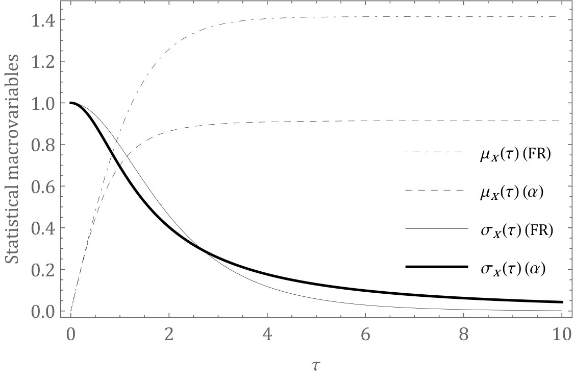 Figure 1
| Metrization | Manifold | IGC growth | IGE growth | Speed of Convergence |
|---|---|---|---|---|
| Fisher-Rao metric | maximally symmetric | exponential | linear | exponential |
| -order metric | isotropic but nonhomogenous | polynomial | logarithmic | polynomial |
Peer Reviews
No public reviews on file for this paper yet. If you reviewed it on a platform where reviews are public (OpenReview, ICLR, NeurIPS, ICML), you can paste yours below so the community can read it here.
Videos
No videos yet. Explain this paper in a talk, walkthrough, or lecture? Add one.
Information Geometric Complexity of Entropic Motion on Curved
Statistical Manifolds under Different Metrizations of Probability Spaces
Steven Gassner and Carlo Cafaro
SUNY Polytechnic Institute, 12203 Albany, New York, USA
Abstract
We investigate the effect of different metrizations of probability spaces on the information geometric complexity of entropic motion on curved statistical manifolds. Specifically, we provide a comparative analysis based upon Riemannian geometric properties and entropic dynamical features of a Gaussian probability space where the two distinct dissimilarity measures between probability distributions are the Fisher-Rao information metric and the -order entropy metric. In the former case, we observe an asymptotic linear temporal growth of the information geometric entropy (IGE) together with a fast convergence to the final state of the system. In the latter case, instead, we note an asymptotic logarithmic temporal growth of the IGE together with a slow convergence to the final state of the system. Finally, motivated by our findings, we provide some insights on a tradeoff between complexity and speed of convergence to the final state in our information geometric approach to problems of entropic inference.
pacs:
Chaos (05.45.-a), Complexity (89.70.Eg), Entropy (89.70.Cf), Inference Methods (02.50.Tt), Information Theory (89.70.+c), Probability Theory (02.50.Cw), Riemannian Geometry (02.40.Ky).
I Introduction
Methods of information geometry amari ; amari2 ; amari3 can be combined with entropic inference techniques caticha12 to quantify the complexity of statistical models used to render probabilistic descriptions of systems about which only limited information is known. Within this hybrid framework, the complexity associated with statistical models can be viewed as a measure of the difficulty of inferring macroscopic predictions due to the lack of complete knowledge about the microscopic degrees of freedom of the system being analyzed cafarophd . Initially, entropic methods can be employed to establish an initial, static statistical model of the complex system. Then, after identifying the microscopic degrees of freedom of a complex system and selecting its relevant information constraints, the statistical model that characterizes the complex system is specified by means of probability distributions parametrized in terms of statistical macrovariables. These variables, in turn, depend upon the specific functional expression of the information constraints assumed to be important for implementing statistical inferences about the system of interest. Once the probability space is endowed with a suitable notion of metric needed to distinguish different elements of the statistical model, one focuses on the evolution of the complex system. Specifically, assuming the complex system evolves, the evolution of the associated statistical model from its initial to final configurations can be determined by means of the so-called Entropic Dynamics (ED, catichaED ).
Entropic Dynamics is a form of information-constrained dynamics on curved statistical manifolds whose elements are probability distributions. Moreover, these distributions are in one-to-one relation with a convenient set of statistical macrovariables that specify a parameter space which provides a parametrization of points on the statistical manifold. The ED setting specifies the evolution of probability distributions in terms of an entropic inference principle:** starting from the initial configuration, the motion toward the final configuration occurs via the maximization of the logarithmic relative entropy functional (Maximum relative Entropy method- MrE method, caticha12 ; adom06 ; adom07 ; adomphd ) between any two consecutive intermediate configurations of the system. ED generates only the expected, but not the actual, trajectories of the system. In this regard, we stress that uncovering links between information geometry and classical Newtonian mechanics can be of great theoretical interest caticha07 ; nico18 . For instance, a formal bridge between information geometric techniques and classical dynamical systems was recently proposed by using the concept of canonical divergence in dually flat manifolds in Ref. nico18 . Inferences within ED rely on the nature of the selected information constraints that are employed at the level of **the MrE algorithm. Modeling schemes of this type can only be validated a posteriori. If discrepancies occur between inferred predictions and experimental observations, a new set of information constraints must be chosen jaynes85 ; dewar09 ; giffin16 . This is an especially important feature of the MrE algorithm and was recently reconsidered in Ref. cafaropre16 by applying entropic inference techniques to stochastic Ising models. The above mentioned entropic maximization procedure specifies the evolution of probability distributions as a geodesic evolution of the statistical macrovariables caticha12 . For recent reviews on an information geometric perspective on the complexity of macroscopic predictions arising from incomplete information, we refer to Refs. ali17 ; felice18 ; ali18 .
A common measure of distance between two different probability distributions is quantified by the Fisher-Rao information metric amari . This distance can be regarded as the degree of distinguishability between two probability distributions. After having determined the information metric, one can apply the usual methods of Riemannian differential geometry to study the geometric structure of the statistical manifold underlying the entropic motion which determines the evolution of the probability distributions. Conventional Riemannian geometric quantities such as Christoffel connection coefficients, the Ricci tensor, the Riemannian curvature tensor, sectional curvatures, scalar curvature, the Weyl anisotropy tensor, Killing fields, and Jacobi fields can be computed in the usual manner thorne73 . Furthermore, the chaoticity (that is, temporal complexity) of such statistical models can be analyzed in terms of convenient indicators, such as: the signs of scalar and sectional curvatures of the statistical manifold, the asymptotic temporal behavior of Jacobi fields, the existence of Killing vectors, and the existence of a non-vanishing Weyl anisotropy tensor. In addition to these measures, complexity can also be quantified** **by means of the so-called information geometric entropy (IGE, ali17 ; felice18 ; ali18 ).
From a theoretical standpoint, the utility of the Fisher-Rao information metric as a suitable distinguishability measure of two probability distribution functions is mainly motivated by Cencov’s theorem cencov ; campbell . This theorem states that the Fisher-Rao information metric is, modulo an unimportant constant factor, the only Riemannian metric that is invariant under mappings referred to as congruent embeddings by Markov morphisms caticha12 . From a computational standpoint, however, the algebraic form of the Fisher-Rao information metric makes it rather difficult to use when applied to multi-parameter spaces like mixture models. For instance, a fundamental drawback of the Fisher-Rao metric is that it is not available in closed-form for a mixture of Gaussians peter06 . These computational inefficiencies extend to the computation of the Christoffel connection coefficients and, therefore, to the integration of geodesic equations. The challenges with the mixture models were originally encountered in the framework of shape matching analysis of medical and biological image structures where shapes are represented by a mixture of probability density functions peter06 . To partially address the above mentioned computational issues, a different Riemannian metric based upon the generalized notion of -entropy functional was employed havrda67 ; burbea82 . The corresponding -order entropy metric allows us to obtain closed-form solutions to both the metric tensor and its derivatives for the Gaussian mixture model. Thus, compared to the Fisher-Rao information metric, the -order entropy metric enhances the computational efficiency in shape analysis tasks peter06 .
In this paper, inspired by the above-mentioned enhanced computational efficiency of the -order entropy metric with respect to the Fisher-Rao information metric, we seek to address the following questions: i) How does a different choice of metrization of probability spaces affect the complexity of entropic motion on a given probability space? ii) Does a possible higher computational efficiency of the -order metric with respect to the Fisher-Rao information metric lead to a lower information geometric complexity of entropic motion? iii) Is there a tradeoff between speed of convergence to the final macrostate and the information geometric complexity of entropic motion?
Our motivation to explicitly compute geometrical quantities including the scalar curvature, the sectional curvature, the Ricci curvature tensor, the Riemann curvature tensor, and the Weyl anisotropy tensor is twofold. First, we wish to present here a comparative analysis of both geometrical and entropic dynamical nature between the Fisher-Rao and the -metrics. Second, in view of possible further investigations concerning the geodesic deviation behavior on curved statistical manifolds along the lines of those presented in Refs. physicad1 ; physicad2 , having the explicit expressions of such geometrical quantities can be quite useful for future efforts. In this respect, for instance, our result concerning the maximal symmetry of the Gaussian probability space endowed with the -metric can have important implications when integrating the Jacobi geodesic spread equation in order to study the deviation of two neighboring geodesics on the manifold casetti . Indeed, for maximally symmetric manifolds, the sectional curvature (that is, the generalization to higher-dimensional manifolds of the usual Gaussian curvature of two-dimensional surfaces) assumes a constant value throughout the manifold. As a result, exploiting this symmetry reduces significantly the otherwise challenging problem of integrating the Jacobi deviation equation by simplifying the differential equation via the expression of the Riemann curvature tensor components that enter it.
The layout of the remainder of the paper is as follows. In Section II, we briefly present the Fisher-Rao information and the -order entropy metrics as special cases of the so-called -entropy metric. In Section III, we describe the information geometric properties of Gaussian probability spaces equipped with the above-mentioned metrizations. In Section IV, we study the geodesics of the entropic motion on the two curved statistical manifolds. In Section V, we report the asymptotic temporal behavior of the information geometric entropy of both statistical models. Our final remarks appear in Section VI. Finally, technical details can be found in Appendix A.
II Metrizations of probability spaces
In this section, we focus on two different metrizations of a probability space. Specifically, we consider the Fisher-Rao information metric and the -order entropy metric. These two metrics are limiting cases of a large class of generalized metrics introduced by Burbea and Rao in Ref. burbea82 .
For a formal mathematical discussion on the -entropy functional formalism, we refer to Ref. burbea82 . In what follows, we present a minimal amount of information concerning this topic needed to follow our work. A -entropy metric is formally defined as the Hessian of a -entropy functional along a direction of the tangent space of the parameter space **. **Note that with and being the dimensionality of the parameter space. Specifically, we have
[TABLE]
with , ,…, , and
[TABLE]
The quantity denotes a -entropy functional, denotes the Hessian of along the direction where repeated indices are summed over, is a generalized convex real-valued -function, is a probability density function, and** is the microspace of the system. The quantity in Eq. (1) can be formally regarded as the second derivative of the function with respect to viewed as an ordinary real-valued variable. In particular, **when is defined as
[TABLE]
we obtain and where the characteristic parameter equals and , respectively. In the former case, reduces to the Fisher-Rao information metric ,
[TABLE]
The quantity** ** in Eq. (4) denotes the relative entropy functional given by caticha12 ,
[TABLE]
In the latter case, becomes the -order metric tensor with given by
[TABLE]
In the next section, we employ the metrics in Eqs. (4) and (6) to measure the distance between probability distributions of a Gaussian statistical manifold.
III Information geometry of a Gaussian statistical model
In this section, we study the information geometry of a two-dimensional probability space specified by Gaussian probability distributions. In the first case, we assume the metrization is defined by the Fisher-Rao information metric in Eq. (4). In the second case, instead, we assume the metrization is given by the -order metric in Eq. (6).
III.1 The Fisher-Rao information metric
Consider a single-variable Gaussian probability density function , given by,
[TABLE]
For a Gaussian distribution, we let , , with and . Therefore, the two-dimensional Gaussian statistical manifold is such that,
[TABLE]
with being the selected metric. Substituting Eq. (7) into Eq. (4), we obtain
[TABLE]
Using the metric tensor components in Eq. (9), we can study a variety of global properties of the two-dimensional Gaussian statistical manifold. For instance, the affine connection coefficients (also known as the Christoffel symbols of second kind) are defined as defelice90 ; weinberg72 ,
[TABLE]
The quantity in Eq. (10) is such that where denotes the Kronecker delta,
[TABLE]
Substituting Eqs. (9) and (11) into Eq. (10), we get
[TABLE]
These connection coefficients in Eq. (12) allow us to quantify the curvature properties of the statistical manifold. Let us first consider the Riemann curvature tensor defelice90 ; weinberg72 ,
[TABLE]
Substituting Eq. (12) into Eq. (13), the non-vanishing Riemann curvature tensor components are
[TABLE]
Furthermore, the Ricci curvature tensor is given by,
[TABLE]
Therefore, using Eqs. (12) and (15), the nonvanishing components of the Ricci tensor are
[TABLE]
Finally, the scalar curvature is defined as
[TABLE]
Therefore, using Eqs. (11) and (16), we obtain
[TABLE]
As a final remark, we recall that the Weyl anisotropy tensor is defined as casetti ,
[TABLE]
with . Substituting Eqs. (14) and (16) into Eq. (19), it happens that the Weyl anisotropy tensor components are identically zero. Moreover, the sectional curvature is constant and equals
[TABLE]
Therefore, being isotropic and homogeneous, the manifold is maximally symmetric. Further technical details on maximally symmetric manifolds appear in Appendix A.
III.2 The -order metric
Consider now a single-variable Gaussian probability density function , as defined in Eq. (7). In what follows, we study the information geometric properties of such a Gaussian probability space by using the -order metric tensor in Eq. (6). Substituting Eq. (7) into Eq. (6), we have
[TABLE]
Using the line of reasoning outlined in the previous subsection, we obtain that the affine connection coefficients are
[TABLE]
Substituting Eq. (22) into Eq. (13), the non-vanishing Riemann curvature tensor components are
[TABLE]
Furthermore, using Eqs. (15) and (22), the nonvanishing components of the Ricci tensor are
[TABLE]
Finally, substituting Eqs. (21) and (24) into Eq. (17), the scalar curvature becomes
[TABLE]
As a final remark, we observe that substituting Eqs. (23) and (24) into Eq. (19), it happens that the Weyl anisotropy tensor components are identically zero. However, the sectional curvature is not constant and equals
[TABLE]
Therefore, being isotropic but not homogeneous, the manifold is not maximally symmetric.
IV Entropic motion
Consider a statistical manifold with a metric . The ED is concerned with the following task catichaED : given the initial and final states, what trajectory is the system expected to follow? The answer happens to be that the expected trajectory is the geodesic that passes through the given initial and final states. Moreover, the trajectory follows from a principle of entropic inference, the MrE algorithm caticha12 ; adom06 ; adom07 ; adomphd . The goal of the MrE method is to update from a prior distribution to a posterior distribution given the information that the posterior lies within a certain family of distributions . The selected posterior is that which maximizes the logarithm relative entropy ,
[TABLE]
We remark that ED is formally similar to other generally covariant theories: the dynamics is reversible, the trajectories are geodesics, the system supplies its own notion of an intrinsic time, the motion can be derived from a variational principle of the form of Jacobi’s action principle rather than the more familiar principle of Hamilton. Roughly speaking, the canonical Hamiltonian formulation of ED is an example of a constrained information-dynamics where the information-constraints play the role of generators of evolution. For further technical details on the ED framework used here, we refer to catichaED .
A geodesic on a -dimensional manifold represents the maximum probability path a complex dynamical system explores in its evolution between initial and final macrostates and , respectively. Each point of the geodesic represents a macrostate parametrized by the macroscopic dynamical variables defining the macrostate of the system. Each component with ,…, is a solution of the geodesic equation catichaED ,
[TABLE]
Furthermore, each macrostate is in a one-to-one correspondence with the probability distribution . This is a distribution of the microstates .
IV.1 The Fisher-Rao information metric
Substituting Eq. (12) into Eq. (28), the two coupled nonlinear second-order ordinary differential equations (ODEs) to consider become
[TABLE]
Let and . Then, the first and the second relations in Eq. (29) become
[TABLE]
respectively. From the first relation in Eq. (30) we observe that
[TABLE]
After some simple algebraic manipulations, we get
[TABLE]
where is an arbitrary constant. Substituting Eq. (32) in the second relation in Eq. (30), we obtain
[TABLE]
We note that by integrating Eq. (33), we find . Then, using Eq. (32), we can obtain an expression for . To simplify the notation, let us set and . Then, Eq. (33) becomes
[TABLE]
To integrate Eq. (34), let us consider a first change of variables
[TABLE]
Substituting Eq. (35) into Eq. (34), we get
[TABLE]
To integrate Eq. (36), let us take into consideration a second change of variables
[TABLE]
Defining , it follows from Eq. (37) that
[TABLE]
since,
[TABLE]
Substituting Eqs. (38) and (37) into Eq.(36), we get
[TABLE]
A simple integration of Eq. (40) yields,
[TABLE]
where and are two real integration coefficients. Recalling that , we deduce from Eq. (41) that
[TABLE]
Observe that,
[TABLE]
Then, upon integration, Eq. (42) yields
[TABLE]
where the integration coefficient . Solving Eq. (44) for , we obtain
[TABLE]
Finally, recalling that , the variance becomes
[TABLE]
It is straightforward to verify that indeed in Eq. (46) satisfies the nonlinear ODE in Eq. (34). From Eq. (32), we find that equals
[TABLE]
Substituting Eq. (46) into Eq. (47), the mean becomes
[TABLE]
where the integration coefficient . As a simplifying working hypothesis, we consider geodesic paths with . Furthermore, we assume that the initial conditions are given by and . These initial conditions imply that and . Finally, letting , the geodesics in Eqs. (46) and (48) become
[TABLE]
and
[TABLE]
respectively. We remark that it is straightforward to check that indeed the expression for and in Eqs. (49) and (50), respectively, satisfy the set of coupled nonlinear ODEs in Eq. (29).
IV.2 The -order metric
Substituting Eq. (22) into Eq. (28), the two coupled nonlinear second-order ODEs to consider become
[TABLE]
Let and . Then, the first and the second relations in Eq. (51) can be rewritten as
[TABLE]
respectively. From the first relation in Eq. (52), we note that
[TABLE]
From Eq. (53), we get
[TABLE]
where is an arbitrary constant. The use of Eq. (54) in the second relation in Eq. (52) yields
[TABLE]
Observe that by integrating Eq. (55), we find . Then, we can obtain an expression for by employing Eq. (54). Setting , Eq. (55) becomes
[TABLE]
To integrate Eq. (56), consider a first change of variables,
[TABLE]
Substituting Eq. (57) into Eq. (56), we get
[TABLE]
To integrate Eq. (58), we perform a second change of variables
[TABLE]
Defining , it follows from Eq. (59) that
[TABLE]
Substituting Eqs. (60) and (59) into Eq.(58), we get
[TABLE]
To integrate Eq. (61), we propose a third change of variables. Let a new variable be defined as,
[TABLE]
Using Eq. (62) and noting that where, with some abuse of notation, , Eq. (61) becomes an ODE of Bernoulli type nagle ,
[TABLE]
To integrate Eq. (63), we introduce a fourth change of variables. Let a new variable be given by,
[TABLE]
Then, using Eq. (64) and noting that with , Eq. (63) becomes
[TABLE]
The most general solution of Eq. (65) is given by,
[TABLE]
where is a real integration coefficient. For the sake of simplicity, we set equal to zero in what follows and, thus,
[TABLE]
Using Eqs. (67), (64), (62), (59), and (57) together with the assumption that , we get
[TABLE]
where we impose with and . Observe that with and in the case of the Fisher-Rao information metric discussed in the previous subsection. At this point, we note that from a formal mathematical standpoint, is such that , where is a phase factor that equals . Therefore, using Eq. (68) and setting , we finally** obtain,**
[TABLE]
Observe that in Eq. (69) and in Eq. (68) satisfy the coupled system of nonlinear ODEs in Eq. (51). To find a closed form analytical solution to the real geodesic equations when the distinguishability between two probability distributions is quantified by means of the -order metric tensor, complex geodesic paths were introduced. Specifically, we employed a nontrivial sequence of suitable change of variables. In order to reverse these operations and return to the original variable, we computed a number of indefinite integrals, each one defined up to a constant of integration. Along the way, we have arbitrarily set equal to zero some of these constants in order to facilitate a return to our starting point with a closed form expression for the geodesics. However, in so doing, we were compelled to obtain a complex solution for the statistical variable . In what follows, we choose as initial conditions and in Eqs. (49), (50), (68), and (69). In this case, in Eq. (69) becomes purely imaginary.
At this juncture, we emphasize that it is not unusual to employ unphysical concepts in intermediate steps to obtaining solutions to problems in theoretical physics peres04 . For example, to characterize a spacelike singularity and an event horizon generated by a black hole in the framework of the AdS/CFT (anti-de-Sitter/conformal field theory) correspondence, it is convenient to study the boundary-to-boundary correlator expressed in terms of an expectation value of two operators (two massive fields, for instance) veronika1 . In general, when evaluating such a boundary correlator, one needs to take into consideration multiple geodesics that connect the two boundary points. In particular, there are scenarios where both real and purely imaginary geodesics can contribute to the computation of the correlation function veronika2 . However, despite subtleties related to the nontrivial mathematical structure of geodesic paths, the boundary correlator can reveal distinct measurable signals of the black hole singularity.
Motivated by these considerations and desiring the have a computationally accessible path leading to an analytical closed form solution of the geodesic trajectories, we allowed for the possibility of considering certain types of* complex*** statistical variables as solutions to the geodesic equation in our information geometric analysis. A couple of remarks are in order. First, we acknowledge that although the expected value of a complex random variable of the form involving two real variables and is a complex number, in our case denotes a real random variable. Therefore, both and assume real values. Second, a rotation in complex analysis is a one-to-one mapping of the -plane onto the -plane such that with being a fixed *real *number. In particular, we note that the moduli and would have the same asymptotic temporal behavior if they are assumed to be time-dependent quantities. Therefore, since we were ultimately interested in evaluating the asymptotic temporal behavior of the information geometric entropy in terms of the moduli of the statistical variables and , we were willing to keep as good solutions either real solutions or complex solutions recast as a complex **constant phase factor times a time-dependent real function to address otherwise intractable computational issues from an analytical standpoint. For the sake of scientific honesty, while searching for our geodesic trajectories, we also give up on any type of generality concerning both initial conditions and functional form of the statistical macrovariables. Therefore, whenever needed, we assumed suitable working assumptions that allowed ultimately to provide a closed form analytical solution for the geodesic equation of the proposed form in Eqs. (68) and (69). We acknowledge this is certainly not the most rigorous approach to our problem. We hope to discover a mathematically rigorous analytical solution to this specific issue in future efforts. For the time being, we emphasize that the temporal behavior of the statistical macrovariables obtained in our analytical computations in Eqs. (49), (50), (68), and (69) is qualitatively consistent with the temporal behavior observed after an approximate numerical integration of the two systems of nonlinear and coupled ODEs in Eqs. (29) and (51). For the sake of conceptual simplicity, instead of using the powerful Runge-Kutta method hildebrand , we employed a forward Euler method Matlab code with step size in our numerics. In particular, we numerically verified that
[TABLE]
that is, approaches its limiting constant value at a rate faster than approaches its terminal constant value. Our numerical results for a special choice of initial conditions are reported in Fig. .
In the next section, we focus on computing the asymptotic temporal behavior of the information geometric entropy constructed in terms of the moduli of the statistical macrovariables in Eqs. (49), (50), (68), and (69). In this manner, in Eq. (69) and its modulus exhibit the same temporal behavior.
V Information Geometric Entropy
In what follows, we briefly present the concept of the IGE. Assume that the points of an -dimensional curved statistical manifold are parametrized in terms of real valued variables ,
[TABLE]
We remark that the microvariables in Eq. (71) are elements of the microspace while the macrovariables in Eq. (71) belong to the parameter space defined as,
[TABLE]
The quantity with in Eq. (72) is a subset of and specifies the entire range of permissible values for the statistical macrovariables . The IGE is a proposed measure of temporal complexity of geodesic paths defined as,
[TABLE]
where the average dynamical statistical volume** ** is given by,
[TABLE]
Note that the operation of temporal average is denoted with the tilde symbol in Eq. (74). Moreover, the volume** **on the RHS of Eq. (74) is defined as,
[TABLE]
where is the so-called Fisher density and equals the square root of the determinant of the metric tensor ,
[TABLE]
We emphasize that the expression of in Eq. (75) can become more transparent for statistical manifolds with metric tensor whose determinant can be factorized in the following manner,
[TABLE]
With the help of the factorized determinant in Eq. (77) , the IGE in Eq. (73) can be rewritten as
[TABLE]
We also stress that the leading asymptotic behavior of is used to characterize the complexity of the statistical models being analyzed. For this reason, it is customary to take into consideration the quantity
[TABLE]
that is to say, the leading asymptotic term in the IGE expression. The integration space in Eq. (75) is defined by
[TABLE]
where with and denoting the initial value of the affine parameter such that,
[TABLE]
The integration domain in Eq. (80) is an -dimensional subspace of whose elements are -dimensional macrovariables with components bounded by given limits of integration and . The integration of the -coupled nonlinear second order ODEs in Eq. (81) determines the temporal functional form of such limits. The IGE at a certain instant is essentially the logarithm of the volume of the effective parameter space explored by the system at that instant. The motivation for considering the temporal average is twofold. In the first case, the temporal average is used in order to smear out (i.e. average) the possibly highly complex fine details of the entropic dynamical description of the system on the manifold. In the second case, the temporal average is used so as to suppress the consequences of transient effects which may enter the computation of the expected value of the volume of the effective parameter space. It is primarily for these two reasons that the the long-term asymptotic temporal behavior is chosen to serve as an indicator of dynamical complexity. In summary, the IGE is constructed to furnish an asymptotic coarse-grained inferential description of the complex dynamics of a system in the presence of only incomplete information. For further technical details on the IGE, we refer to Refs. ali17 ; felice18 ; ali18 .
In this section, we wish to compute the asymptotic temporal behavior of the** **information geometric complexity defined as,
[TABLE]
where , and .
V.1 The Fisher-Rao information metric
We are interested in the entropic motion from to with and . Assuming the initial condition and using Eqs. (49) and (50), we get
[TABLE]
The quantity in Eq. (83) is . Furthermore, using Eq. (9), the asymptotic temporal behavior of the information geometric complexity in Eq. (82) becomes
[TABLE]
Using Eq. (83), Eq. (84) yields
[TABLE]
After some algebra, we obtain
[TABLE]
that is,
[TABLE]
Equation (87) exhibits asymptotic linear temporal growth of the information geometric entropy of the statistical model .
V.2 The -order metric
As previously stated, we are interested in the entropic motion from to with and . Assuming the initial condition and using Eqs. (68) and (69), we find
[TABLE]
The quantity in Eq. (88) is with and (that is, with ). Furthermore, using Eq. (21), in Eq. (82) becomes
[TABLE]
Using Eq. (88), Eq. (89) yields
[TABLE]
After some algebra, we get
[TABLE]
with in Eq. (91) defined as , that is
[TABLE]
Eq. (92) exhibits the asymptotic logarithmic temporal growth of the information geometric entropy of the statistical model .
VI Final Remarks
In this paper, we investigated the effect of distinct metrizations of probability spaces on the information geometric complexity of entropic motion on curved statistical manifolds. Specifically, we considered a comparative analysis based upon Riemannian geometric properties and entropic dynamical features of a Gaussian probability space where the two dissimilarity measures between probability distributions were the Fisher-Rao information metric (see Eq. (4)) and the -order entropy metric (see Eq. (6)). In the former case, we noticed an asymptotic linear temporal growth of the IGE (see Eq. (87)) together with a fast convergence to the final state of the system (see Eq. (83)). By contrast, in the latter case we observed an asymptotic logarithmic temporal growth of the IGE (see Eq. (92)) together with a slow convergence to the final state of the system (see Eq. (88)). Our main results are summarized in Fig. 1 together with Table I and can be outlined as follows.
We demonstrated that while is a maximally symmetric curved statistical manifold with constant sectional curvature (see Eq. (20)), the manifold is not maximally symmetric since it is isotropic and nonhomogeneous (see Eq. (26)). 2. 2.
We found that the geodesic motion on exhibits a fast convergence toward the final macrostate with with (see Eq. (83)). Instead, the geodesic motion on shows a slow convergence toward the final macrostate with (see Eq. (88)). 3. 3.
We determined that the IGE exhibits an asymptotic linear and logarithmic temporal growth in the case of and , respectively. These findings appear in Eqs. (87) and (92), respectively.
In addition to having a relevance of its own, our findings can be relevant to a number of open problems. For instance, thanks to our geodesic motion analysis together with the observed link between the information geometric complexity and the speed of convergence to the final state, our work appears to be useful for deepening our limited understanding about the existence of a tradeoff between computational speed and availability loss in an information geometric setting of quantum search algorithms with a thermodynamical flavor as presented in Refs. cafaro17 ; cafaro18 . Furthermore, in view of our study of the geometrical and dynamical features that emerge from distinct metrizations of probability spaces, our comparative analysis can help investigate the unresolved problem of whether the complexity of a convex combination of two distributions is related to the complexities of the individual constituents ay09 . Indeed, unlike the Fisher-Rao information metric, the -order metric is available in closed form for Gaussian mixture models peter06 . We leave the exploration of these intriguing topics of investigation to future scientific efforts. We also emphasize that our information geometric analysis shares some resemblance with quantum cosmological investigations. First, we observe that the connection coefficients appearing in our information geometric investigation arise from a symmetric connection (i.e. , where denotes the components of the torsion tensor capozziello01 ). In principle however, we could incorporate non-vanishing torsion in our information geometric framework. The inclusion of torsion could relate in a natural manner to quantum mechanics given the noncommutative nature of its underlying probabilistic structure. In particular, given the findings described in our paper, an investigation of the transition from isotropic to anisotropic features in cosmological models equipped with torsion capozziello17 would constitute an intriguing line of exploration in future information geometric efforts where we quantify the complexity of statistical models (both isotropic and anisotropic) under different metrizations. Second, it can be shown in quantum cosmology that a nonzero cosmological constant can emerge by virtue of using the von Neumann entropy in cosmological toy models to quantify statistical correlations between two distinct cosmic epochs (i.e., entanglement between quantum states) capozziello13 ; capozziello11 ; capozziello13b . In view of the use of entropic tools to model, investigate and understand the link between statistical correlations and quantum entanglement, the aforementioned quantum cosmological line of research bears a high degree of similarity with our information geometric complexity characterization of quantum entangled Gaussian wave packets as presented in Refs. kim11 ; kim12 .
Although our considerations are mainly speculative at this time, we hope to enhance our understanding of the link between quantum cosmological models and information geometric statistical models in our forthcoming scientific efforts.
Acknowledgements.
C. C. acknowledges the hospitality of the United States Air Force Research Laboratory (AFRL) in Rome-NY where part of his contribution to this work was completed. Finally, constructive criticism from an anonymous referee leading to an improved version of this manuscript are sincerely acknowledged by the authors.
Appendix A Maximally symmetric manifolds
A maximally symmetric manifold must be homogeneous and isotropic defelice90 ; weinberg72 . Homogeneity implies invariance under any translation along any coordinate axis. Isotropy, instead, implies invariance under rotation of any coordinate axis into any other coordinate axis. In what follows, we study the properties of an -dimensional maximally symmetric manifold in terms of its independent Killing vectors. In particular, we identify the expressions of the scalar curvature together with the Ricci and Riemann curvature tensors for a maximally symmetric manifold. It happens that while the homogeneity of the manifold can be expressed in terms of the behavior of the scalar curvature, the isotropy feature is encoded in the behavior of the Ricci and Riemann curvature tensors. In what follows, we use Greek letters to describe the indices of tensorial components.
In terms of the concept of covariant derivative, the Riemann curvature tensor is defined as
[TABLE]
where denotes an arbitrary vector field, is the commutator, and is given by
[TABLE]
When the vector field is chosen to be a Killing vector , Eq. (93) becomes
[TABLE]
More specifically, however, Killing vectors satisfy the following equation
[TABLE]
From the associativity of covariant derivatives, we obtain
[TABLE]
Using Eq. (96) and the product rule, Eq. (97) becomes
[TABLE]
that is,
[TABLE]
From Eq. (97), we also have
[TABLE]
that is, using the product rule,
[TABLE]
so that
[TABLE]
Using Eq. (93), Eq. (102) becomes
[TABLE]
Recalling that the commutator of two constant vectors is zero, Eq. (103) yields
[TABLE]
Equating Eq. (99) and Eq**.** (104), we obtain
[TABLE]
that is,
[TABLE]
Since Killing vectors satisfy the relation , introducing the Kronecker delta, Eq. (106) can be recast as
[TABLE]
In general, the quantities and cannot be prescribed independently. However, when a manifold is maximally symmetric and admits all the allowed Killing forms, the quantities and can be prescribed independently. In order for the sets and to be independently specifiable, we impose
[TABLE]
and,
[TABLE]
For an -dimensional curved manifold, a suitable sequence of tensor algebra manipulations of Eq. (109) leads to the following expressions of the Ricci and the Riemann curvature tensors,
[TABLE]
respectively. In Eq. (110), and denote the metric tensor and the scalar curvature of the manifold, respectively. Finally, using the second relation in Eq. (110) together with a convenient sequence of tensor algebra manipulations, Eq. (108) yields
[TABLE]
Eq. (111) implies that the scalar curvature must be covariantly constant for a maximally symmetric manifold. The relations in Eq. (110) are valid for an isotropic manifold while Eq. (111) holds true for a homogeneous manifold. For a maximally symmetric manifold, both Eqs. (110) and (111) must hold true.
We point out that instead of using Eq. (93), it is possible to define the Riemann curvature tensor by the relation
[TABLE]
In this case, the Riemannian curvature tensor components have the opposite sign compared to those defined in Eq. (94). In particular, in this case the second relation in Eq. (110) becomes
[TABLE]
As a final remark, we recall that the Weyl anisotropy tensor is defined as casetti ,
[TABLE]
In the working assumption of an isotropic manifold, using the first relation in Eq. (110) and contracting with , we** **obtain
[TABLE]
that is, by means of Eq. (113),
[TABLE]
From Eq. (116), we conclude that the Weyl anisotropy tensor vanishes in the case of an isotropic manifold.
The reference list from the paper itself. Each links out to its DOI / PubMed record.
- 1(1) S. Amari and H. Nagaoka, Methods of Information Geometry , Oxford University Press (2000).
- 2(2) S. Amari, Differential-Geometric Methods in Statistics , vol. 28 of Lecture Notes in Statistics, Springer-Verlag (1985).
- 3(3) S. Amari, Information Geometry and Its Applications , Springer-Japan (2016).
- 4(4) A. Caticha, Entropic Inference and the Foundations of Physics ; USP Press: São Paulo, Brazil, 2012; Available online: http://www.albany.edu/physics/A Caticha-EIFP-book.pdf.
- 5(5) C. Cafaro, The Information Geometry of Chaos , Ph.D. Thesis in Physics, State University of New York, Albany, NY, USA (2008).
- 6(6) A. Caticha, Entropic dynamics , AIP Conf. Proc. 617 , 302 (2002).
- 7(7) A. Caticha and A. Giffin, Updating probabilities , AIP Conf. Proc. 872 , 31 (2006).
- 8(8) A. Giffin and A. Caticha, Updating probabilities with data and moments , AIP Conf. Proc. 954 , 74 (2007).