Continuous-time quantum search and time-dependent two-level quantum systems
Carlo Cafaro, Paul M. Alsing

TL;DR
This paper explores the connection between quantum search algorithms and exactly solvable time-dependent two-level quantum systems, providing analytical results on transition probabilities and their relation to search strategies.
Contribution
It establishes a detailed analytical link between quantum search Hamiltonians and solvable two-level systems, analyzing transition behaviors and their implications for search algorithms.
Findings
Exact analytical transition probabilities for time-dependent two-level systems.
Identification of oscillatory and monotonic behaviors related to search algorithms.
Insights into the control of quantum search processes via time-dependent Hamiltonians.
Abstract
It was recently emphasized by Byrnes, Forster, and Tessler [Phys. Rev. Lett. 120, 060501 (2018)] that the continuous-time formulation of Grover's quantum search algorithm can be intuitively understood in terms of Rabi oscillations between the source and the target subspaces. In this work, motivated by this insightful remark and starting from the consideration of a time-independent generalized quantum search Hamiltonian as originally introduced by Bae and Kwon [Phys. Rev. A 66, 012314 (2002)], we present a detailed investigation concerning the physical connection between quantum search Hamiltonians and exactly solvable time-dependent two-level quantum systems. Specifically, we compute in an exact analytical manner the transition probabilities from a source state to a target state in a number of physical scenarios specified by a spin-1/2 particle immersed in an external time-dependent…
Click any figure to enlarge with its caption.
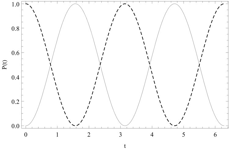 Figure 1
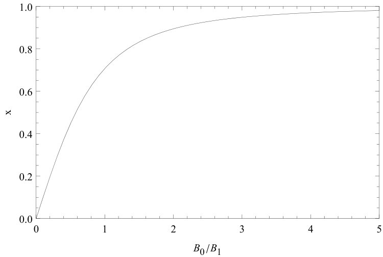 Figure 2
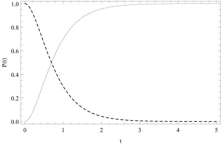 Figure 3
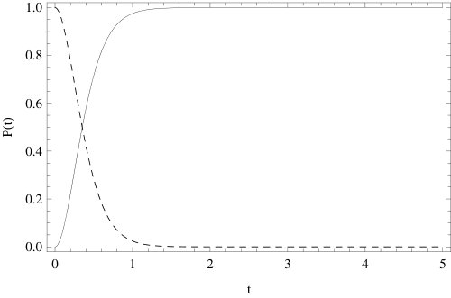 Figure 4
| Hamiltonians | Energy gap | Interaction strength | Characteristic frequency | Angular frequency | Search time |
|---|---|---|---|---|---|
| Rabi | |||||
| Farhi-Gutmann |
| Speed of the schedule | Fixed-point property | Grover-like scaling |
|---|---|---|
| no | no | |
| yes | no | |
| no | yes | |
| yes | no | |
| yes | yes |
Peer Reviews
No public reviews on file for this paper yet. If you reviewed it on a platform where reviews are public (OpenReview, ICLR, NeurIPS, ICML), you can paste yours below so the community can read it here.
Videos
No videos yet. Explain this paper in a talk, walkthrough, or lecture? Add one.
Continuous-time quantum search and time-dependent two-level quantum
systems
Carlo Cafaro1 and Paul M. Alsing2
1SUNY Polytechnic Institute, 12203 Albany, New York, USA
2Air Force Research Laboratory, Information Directorate, 13441 Rome, New York, USA
Abstract
It was recently emphasized by Byrnes, Forster, and Tessler [Phys. Rev. Lett. 120, 060501 (2018)] that the continuous-time formulation of Grover’s quantum search algorithm can be intuitively understood in terms of Rabi oscillations between the source and the target subspaces.
In this work, motivated by this insightful remark and starting from the consideration of a time-independent generalized quantum search Hamiltonian as originally introduced by Bae and Kwon [Phys. Rev. A 66, 012314 (2002)], we present a detailed investigation concerning the physical connection between quantum search Hamiltonians and exactly solvable time-dependent two-level quantum systems. Specifically, we compute in an exact analytical manner the transition probabilities from a source state to a target state in a number of physical scenarios specified by a spin- particle immersed in an external time-dependent magnetic field. In particular, we analyze both the periodic oscillatory as well as the monotonic temporal behaviors of such transition probabilities and, moreover, explore their analogy with characteristic features of Grover-like and fixed-point quantum search algorithms, respectively. Finally, we discuss from a physics standpoint the connection between the schedule of a search algorithm, in both adiabatic and nonadiabatic quantum mechanical evolutions, and the control fields in a time-dependent driving Hamiltonian.
pacs:
Quantum computation (03.67.Lx), Quantum information (03.67.Ac).
I Introduction
The first continuous-time version of Grover’s original discrete quantum search algorithm was proposed by Farhi and Gutmann in Ref. farhi98 . In particular, a generalization of the Farhi-Gutmann analog quantum search algorithm was considered by Bae and Kwon in Ref. bae02 . Both quantum search Hamiltonians in Refs. farhi98 ; bae02 are time-independent. The transition from time-independence to time-dependent in the framework of analog quantum search algorithms appears originally under the working assumption of global adiabatic evolution in Ref. farhi00 and later, in the more advantageous setting of local adiabaticity in Ref. roland02 . In the local adiabatic evolution approach, the time-dependent search Hamiltonian is the linear interpolation between two time-independent Hamiltonians. Specifically, the system is prepared in the ground state of one of the two Hamiltonians. Then, this Hamiltonian is adiabatically changed into the other one whose ground state is assumed to encode the unknown solution of the search problem. The time-dependence of the Hamiltonian is encoded in the time-dependent interpolation function. In particular, the precise form of such a function can be determined by imposing the local adiabaticity condition at each instant of time during the quantum mechanical evolution of the system. Roughly speaking, the adiabatic approximation states that a system prepared in an instantaneous eigenstate of the Hamiltonian will stay close to this prepared state if the Hamiltonian changes sufficiently slowly sanders04 ; oh05 . Therefore, any functional form of the interpolation schedule that satisfies the necessary degree of slowness for the adiabatic condition to be fulfilled can be formally considered. We emphasize that** **there is no fundamental reason to exclude a nonlinear interpolation of the two static Hamiltonians ali04 . Indeed, Perez and Romanelli considered nonadiabatic quantum search Hamiltonians specified in terms of a nonlinear interpolation of the two time-independent Hamiltonians in Ref. romanelli07 . Depending on both the parametric and temporal form of the two interpolation functions used to define the time-dependent Hamiltonian, they presented two search algorithms exhibiting different features. In particular, while both of them exhibited the typical Grover-like scaling behavior in finding the target state in an -dimensional search space, one of the algorithms required a specific time to make the measurement and find the target state (periodic oscillatory behavior and original Grover search algorithm, grover97 ; cafaro12a ; cafaro12b ). The other one, instead, caused the source state to evolve asymptotically into a quantum state that overlapped with the target state with high probability (monotonic behavior and fixed-point Grover search algorithm, grover05 ; cafaro17 ).
Recently, Dolzell, Yoder, and Chuang investigated in detail the possibility for adiabatic quantum search algorithms to exhibit the fixed-point property in addition to quadratic quantum speedup dalzell17 . From their theoretical analysis, supported by a number of illustrative examples, they concluded that depending on the choice of the interpolation schedule of the algorithm, it is possible to construct quantum search Hamiltonians with a variety of features: Grover-like scaling and fixed-point property; Grover-like scaling but no fixed-point property; fixed-point property but no Grover-like scaling. It is especially relevant to our present work to recognize** **that their theoretical investigation was deeply influenced by the intuition that a two-dimensional system whose dynamics is governed by a time-dependent Hamiltonian is essentially equivalent to a spin- particle subject to an external time-dependent magnetic field. This link between the quantum dynamics of a spin- particle in an external magnetic field and quantum search algorithms was further discussed by Byrnes, Forster, and Tessler in Ref. byrnes18 . In this work, the authors point out that Grover’s original quantum search algorithm occurs in the setting of discrete variable quantum computing and, in particular, the Grover operator only inverts the sign to one state. In the framework of quantum computing with continuous variables where the units of quantum information are called qunats braunstein05 , changing a phase to simply a single quantum subspace of an infinite-dimensional Hilbert space implies that the Grover operator would have to invert the phase of an infinitely squeezed momentum state pati00 . This task presents two drawbacks: first, it is difficult to prepare such a state from an experimental standpoint; second, this infinitely squeezed momentum state would have no quantum mechanical overlap with the solution states encoded in the position eigenstates. Motivated by these considerations, Byrnes, Forster, and Tessler present in Ref. byrnes18 a continuous-time generalization of Grover’s original quantum search algorithm where not only the Oracle operator inverts the phase of an arbitrary number of target states but the Grover operator also inverts the sign to an arbitrary number of quantum states. In particular, they pointed out that Grover’s search Hamiltonian can be intuitively understood in terms of Rabi oscillations between the source and the target subspaces.
In this paper, inspired by the analogy discussed in Ref. byrnes18 , we seek to provide a unifying perspective on the above mentioned different types of analog quantum search algorithms in terms of the quantum mechanics of two-level quantum systems. In particular, beginning from the analysis of a time-independent generalized quantum search Hamiltonian as originally introduced in Ref. bae02 , we present a detailed investigation concerning the physical connection between quantum search Hamiltonians and exactly solvable time-dependent, two-level quantum systems. Specifically, we analytically calculate the transition probabilities from a source state to a target state in a number of physical scenarios specified by a spin- particle immersed in an external time-dependent magnetic field. In particular, we analyze the observed periodic oscillatory and monotonic temporal behaviors of such transition probabilities and investigate their analogy with characterizing features of Grover-like and fixed-point quantum search algorithms, respectively. Finally, we discuss the physical link between the schedule of a search algorithm, in both adiabatic and nonadiabatic quantum mechanical evolutions, and the control fields in a driving time-dependent Hamiltonian.
The layout of the remainder of the paper is as follows. In Section II, we examine the transition probability from a source state to a target state for a two-level quantum system whose time-independent Hamiltonian evolution was originally considered by Bae and Kwon in Ref. bae02 . In Section III, we transition from time-independent to time-dependent Hamiltonians. Specifically, we discuss the temporal behavior of the transition probability from a source state to a target state for a two-level quantum system immersed in a time-dependent external magnetic field configuration that specifies the original scenario considered by Rabi in Ref. rabi37 . The explicit computations leading to uncover the exact temporal behavior of both quantum mechanical probability amplitudes and transition probabilities as presented in Sections II and III (and, in a more detailed fashion, in Appendices A and C, respectively) allow us to strengthen the original intuitions reported in Refs. dalzell17 ; byrnes18 . These results also enable a transparent comparison between the dynamics generated by a time-independent Grover-like quantum search Hamiltonian and a time-dependent Rabi-like two-level quantum Hamiltonian. In Section IV, we present the basic notions of adiabatic and nonadiabatic quantum search Hamiltonians. In the adiabatic case, we emphasize the intuitive link between the dynamics generated by quantum search Hamiltonians and the non-relativistic quantum mechanical dynamics of an electron in an external time-dependent magnetic field. In the nonadiabatic case, instead, we focus on the temporal behavior of the transition probabilities from a source state to a target state under suitable working assumptions on the schedules of the nonadiabatic search Hamiltonian. In Section V, upon relaxing the working assumption of knowing a priori the exact time-dependent external magnetic field configuration, we study two quantum dynamical evolution scenarios specified by suitable time-dependent magnetic field configurations (determined a posteriori) that produce transition probabilities showing a temporal monotonic convergence from the source to the target states. In the former scenario we assume that the phase and the magnitude of the transverse field are interconnected. In the latter scenario, while preserving the same formal expression of the complex transversal field, we do not assume any connection between the phase and the intensity of the field itself. Finally, exploiting the analogies between the dynamics generated by a time-independent Grover-like quantum search Hamiltonian and a time-dependent Rabi-like two-level quantum Hamiltonian presented in Sections II and III, a comparison between the dynamics of the newly selected time-dependent Hamiltonians and that of nonadiabatic quantum search Hamiltonians with a fixed-point property is presented. Our final remarks appear in Section VI. Several technical details are presented in the Appendices A, B, C, D, and E.
II A time-independent quantum search Hamiltonian
Consider the time-independent generalized quantum search (GQS) Hamiltonian defined as bae02 ,
[TABLE]
where , , , are complex expansion coefficients. Furthermore, assume that the quantum state is the normalized target state while is the normalized initial state with real quantum overlap that evolves in an unitary fashion according to Schrödinger’s quantum mechanical evolution law,
[TABLE]
with denoting the reduced Planck constant. Our goal is to compute the time such that where is the transition probability defined as,
[TABLE]
Employing the Gram-Schmidt orthonormalization technique, we can construct an orthonormal set of state vectors starting from the set . We obtain,
[TABLE]
Let us define the quantum state vector as,
[TABLE]
Recalling that , Eq. (5) becomes
[TABLE]
In terms of the orthonormal basis , the state becomes
[TABLE]
Note that the quantum overlap is given by,
[TABLE]
Therefore, by** **employing Eq. (8), the state in Eq. (7) can be written as
[TABLE]
After a straightforward but tedious computation, we find that the transition probability in Eq. (3) becomes
[TABLE]
where , , , and are defined as,
[TABLE]
A detailed derivation of Eq. (10) appears in Appendix A. From Eq. (10), it follows that the maximum of occurs at the instant ,
[TABLE]
and, in addition, is equal to
[TABLE]
Finally, using Eq.(11) and observing that and must be real coefficients while , in Eq. (12) and in Eq. (13) become
[TABLE]
and,
[TABLE]
respectively. For the sake of completeness, we point out that in the limiting case of and , we recover the original Farhi-Gutmann (FG) results,
[TABLE]
Moreover, we also recover the transition probability ,
[TABLE]
It is insightful to point out that the minimum search time in Eq. (12) needed to achieve the maximal success probability in Eq. (13) is inversely proportional to the energy level separation where denote the two real eigenvalues of the Hermitian matrix ,
[TABLE]
Therefore, it appears reasonable from our analysis that the finiteness of the minimum search time can be explained in terms of the familiar phenomenon of avoided level crossing in quantum perturbation theory landau . Such a phenomenon is caused by the effect of an external perturbation on a two-level quantum system. Specifically, the two energy levels move apart in opposite direction after applying the perturbation. The higher level increases while the lower level decreases. Furthermore, the energy splitting is more prominent when the unperturbed Hamiltonian is degenerate. This link between analog quantum search algorithms and perturbations in quantum theory will be further explored in the next sections.
III Periodic oscillatory behavior and the Rabi time-dependent
Hamiltonian
In this section, we begin by computing the transition probability from a source state to a target state for a two-level quantum system immersed in a time-dependent external magnetic field configuration that characterizes the original scenario considered by Rabi in Ref. rabi37 . For a brief review on the concept of interaction representation in quantum mechanics in the context of time-dependent perturbations, we refer to Appendix B.
III.1 Transition probability: General setting
The general expression of the time-dependent Hamiltonian of the system that we are investigating is given by,
[TABLE]
In particular, to study the original scenario considered by Rabi in Ref. rabi37 , assume that the time-independent free Hamiltonian and the time-dependent interaction potential are defined as sakurai ,
[TABLE]
respectively. The two parameters and are positive and real. Furthermore, we assume that and for any , . Using Eqs. (136) and (20), we obtain
[TABLE]
that is,
[TABLE]
where for any , and denotes the characteristic frequency of the two-level system. The matrix equality in Eq. (22) yields a system of two coupled first order ordinary differential equations,
[TABLE]
At this point, we recall that the transition probabilities and are defined as and , respectively. After some algebra (for more details, we refer to Appendix C), we find that the transition probabilities and are given by
[TABLE]
and,
[TABLE]
respectively. In Fig. 1, we report the oscillatory and periodic temporal behavior of the transition probabilities and at the original Rabi resonance where with , , and . For the sake of completeness, observe that
[TABLE]
where the quantum state is such that,
[TABLE]
with .
III.2 Time-dependent magnetic field in the Rabi Hamiltonian
At this point, in an effort to emphasize several physics insights between analog quantum search algorithms and time-dependent Hamiltonians, we recall that the most general time-dependent Hermitian Hamiltonian operator with a -matrix representation can be recast as,
[TABLE]
where denotes the vector of Pauli matrices, is the identity operator, is a time-dependent function, and is the vector given by
[TABLE]
Recalling that the Pauli vector operator is defined as cafaro10 ; cafaro14 ,
[TABLE]
we note that the matrix representation of the Hamiltonian in Eq. (28) with respect to the canonical basis is given by,
[TABLE]
For the sake of notational simplicity, we have omitted to make explicit the time-dependence of the scalar function and the vector in Eq. (28). The Rabi-like Hamiltonian in Eq. (19) can be rewritten as,
[TABLE]
where the vector denotes the external time-dependent magnetic field with constant magnitude,
[TABLE]
with , , and the angular frequency belonging to . The vector operator is the magnetic moment of the electron,
[TABLE]
with being the electric charge of the electron, is its mass, and denotes the speed of light. Finally, the quantity denotes the Bohr magneton.
We point out that in Eq. (32) is not only time-dependent but, in general, the Hamiltonian at two different instances does not commute,
[TABLE]
where . For instance, taking and and recalling the commutation relations between the Pauli matrices sakurai ; picasso ,
[TABLE]
we obtain,
[TABLE]
Fundamentally, Eq. (35) is a consequence of the fact that in the original Rabi scenario, although the amplitude of the magnetic field is stationary, the direction of this field does change in time.
III.3 Comparison between the Rabi and the Farhi-Gutmann Hamiltonians
Having introduced the magnetic field and the magnetic moment , the connection between in Eq. (19) and in Eq. (32) becomes clear once one considers the following correspondences,
[TABLE]
A schematic correspondence between selected features that characterize the quantum dynamics arising from the Rabi and the Farhi-Gutmann Hamiltonians appear in Table I. In particular, equating the energy gaps and the interaction strengths in the two frameworks, it follows that
[TABLE]
A plot of Eq. (39) appears in Fig. . Having pointed out these correspondences, we also remark that in Eq. (32) can be written as
[TABLE]
where and are given by,
[TABLE]
and,
[TABLE]
respectively. Note that in Eq. (41) does not depend on time while the unit vector becomes time-independent only if is set equal to zero. In the remainder of this section, in order to facilitate discussion of the formal comparison between Grover-like time-independent quantum search Hamiltonians and Rabi-like time-dependent two-levels Hamiltonians, we focus without any loss of generality on the original Farhi-Gutmann Hamiltonian. In particular, before comparing the transitions probabilities in Eqs. (10) and (25), inspired by the Hamiltonian decomposition as presented in Eq. (19), we note that the original Farhi-Gutmann Hamiltonian can be formally written as
[TABLE]
where . In addition, the states and replace the states and , respectively. The Hamiltonians and in Eq. (43) are given by,
[TABLE]
and,
[TABLE]
respectively. From Eqs. (19), (44), and (45), we note that
[TABLE]
From Eq. (46), the energy gap and, furthermore, the characteristic frequency of the two-level system becomes
[TABLE]
In particular, using Eqs. (25) and (38) it can be shown that at resonance, that is when , the analogue of Eq. (16) obtained in the original Farhi-Gutmann framework becomes
[TABLE]
Having pointed out these formal correspondences between the two quantum dynamical scenarios in Eqs. (46) and (47), we conclude by emphasizing the formally identical periodic oscillatory temporal behavior in the transition probabilities obtained in Eqs. (10) and (25).
Despite these formal analogies between the Grover-like and the Rabi-like scenarios, the spin- particle can be regarded as immersed in a stationary magnetic field in the former case while it is subject to a time-dependent magnetic field configuration in the latter one. For this reason, we observe distinctive features in the two scenarios, both in the mathematical methods employed (mathematical physics) and in the type of perturbation of the quantum system (quantum physics). From a mathematical physics standpoint, instead of using familiar matrix algebra methods and finding an explicit expression for the unitary temporal evolution operator as we did in the first scenario, we were compelled to employ the integration of ODEs approach to determine the probability amplitudes in the second quantum dynamical setting specified by a non-stationary magnetic field configuration (with constant amplitude but time-dependent direction) assumed to be known** a priori. **Unfortunately, the possibility of solving in an exact analytical fashion these systems of coupled linear ODEs with time-dependent coefficients is rather unusual. From a quantum physics standpoint, when transitioning from the first to the second scenario, we go from a time-independent to a time-dependent perturbation. In the latter scenario, recalling the considerations on the link between anticrossing and minimum search time pointed out at the end of Section I, one can think of changing the perturbation by suitably varying the magnetic field amplitude and/or its frequency in order to minimize the search time. Interestingly, the passage through resonance, either by adiabatically varying the magnetic field or the frequency, occurs in magnetic resonance phenomena. Thus, motivated by the remarkable insights presented in Ref. byrnes18 , we proposed in Sections II and III a link between the physics of two-level quantum systems and analog quantum search algorithms. This link, emphasizing the role played by perturbations, leads naturally to the consideration of the concept of adiabaticity in Section IV.
The** **next section serves as a bridge between Section III and Section V. In the latter section, we shall investigate the possibility of finding suitable magnetic field configurations yielding transition probabilities with a monotonic temporal behavior that one would observe in a quantum dynamical evolution under a fixed-point quantum search Hamiltonian. In Section IV, we shall revisit the concepts of adiabatic and nonadiabatic quantum search algorithms.
IV Adiabatic and nonadiabatic quantum search
The intuitive analogy between the quantum evolution of a spin- particle in an external magnetic field and the dynamics arising from a time-dependent Hamiltonian of a two-level quantum system was originally exploited in the context of fixed-point adiabatic quantum search by Dalzell, Yoder, and Chuang in Ref. dalzell17 . For the sake of transparency, we point out that no explicit temporal behavior of transition probabilities was considered by these authors. On the contrary, such a temporal dependence was investigated in two dynamical scenarios proposed by Perez and Romanelli in the framework of nonadiabatic quantum search in Ref. romanelli07 . It is worth noting however, no physical connection between the quantum search Hamiltonians and the driven time-dependent two-level quantum systems was addressed by these latter authors.
In what follows, motivated by our physical insights presented in Sections II and III, we revisit the basic concepts of adiabatic and nonadiabatic quantum search algorithms. The review of both adiabatic and nonadiabatic quantum search algorithms together with the material that will be introduced in Section V will help us establish a physical link between the schedule of a search algorithm and the control fields that specify a time-dependent driving Hamiltonian.
IV.1 The adiabatic framework
The quantum mechanical evolution in the case of adiabatic quantum search can be described in terms of a time-dependent Hamiltonian specified by means of a linear interpolation of two time-independent Hamiltonians farhi00 ; roland02 ,
[TABLE]
where , , and . For the sake of completeness, we remark that there is no fundamental reason why one could not consider a nonlinear interpolation of Hamiltonians in Eq. (49). For more details on the possibility of considering a nonlinear interpolation when , we refer to Ref. ali04 . The time-dependent function that defines the linear interpolation is a smooth function such that and , with being the run time of the search algorithm. Stated otherwise, the functions and denote a turn-on and a turn-off function, respectively. The basic idea in the adiabatic quantum search algorithm can be expressed as follows. Assuming that the ground state of the Hamiltonian encodes the solution of the search problem, to find the target state with large probability, we prepare the system in the ground state of the Hamiltonian . Then, we change adiabatically to from to . The fulfillment of the adiabaticy condition determines the possible temporal expressions of the function . In particular, adapting the evolution rate to the local adiabaticity condition
[TABLE]
Roland and Cerf obtained the following optimum expression of in Ref. roland02 ,
[TABLE]
The quantity in Eq. (50) is the energy gap between the ground state and the first excited state of the Hamiltonian while the real parameter is such that . We remark that the reduced Planck constant is set equal to one in Eq. (50) so that has the physical dimensions of an energy with joules equal to seconds*-1* since . Note that imposing in Eq.(51), in the limit of approaching infinity with and being the dimensionality of the search space, we can obtain the typical Grover-like scaling behavior (for instance, see the first relation in Eq. (16)),
[TABLE]
The method used by Dalzell, Yoder, and Chuang to establish whether or not a given adiabatic quantum search Hamiltonian possesses the fixed-point property was developed by exploiting a physics intuition. Specifically, they noted that the quantum search Hamiltonian in Eq. (49) can be formally viewed as a Hamiltonian describing the quantum evolution of a spin- particle (an electron, for instance) in an external magnetic field. Then, using a Bloch sphere geometric description, the evolution of the quantum state of the system can be described as a spin precessing on the sphere around the magnetic field vector at a temporal rate proportional to the magnitude of the field itself. At the beginning, the source state (that is, the spin of the particle at ) and the magnetic field vectors are parallel. At the end of the evolution, while the magnetic field vector is parallel to the target state , the final state at (that is, the spin of the particle at ) is only approximately parallel to . If the search algorithm has a fixed-point property, then there must exist an upper bound on the angle between and . The existence of such an upper bound was estimated, in certain scenarios, by Dalzell, Yoder, and Chuang in Ref. dalzell17 thanks to the above mentioned geometric description of physical origin together with clever sequences of time-dependent change of coordinates to study the quantum mechanical Schrödinger evolution.
We briefly recall that in Grover’s original search scheme, the algorithm must be stopped at a precise instant in order to have a large success probability. Instead, a search algorithm shows a fixed-point property when the transition probability from the source state to the target state remains high even when the algorithm runs longer than necessary. In Ref. dalzell17 , the authors consider algorithms specified by schedules parametrized in terms of two real parameters and . The former parameter quantifies how fast the interpolation between the two static Hamiltonians occurs, while** **the latter is a lower bound on the fraction of target states with . Observe that denotes the number of target states while is the dimensionality of the Hilbert search space. The algorithm has a Grover-like scaling if the run time is , that is, there exists positive constants and such that
[TABLE]
for any . Furthermore, the algorithm has a fixed-point property if there exists a function such that,
[TABLE]
for all and approaches zero as goes to zero.
Depending on the choice of the schedule , Dalzell, Yoder, and Chuang were able to find a variety of types of search algorithms: some algorithms have both Grover-like scaling and fixed-point property, some have Grover-like scaling but are not fixed-point, and some are fixed-point but lack Grover-like scaling. For example, algorithms defined by means of a schedule with a temporal rate of change proportional to the second power of the energy gap like the one in Ref. roland02 exhibit both a Grover-like scaling and a fixed-point property. For an overview of the various scenarios covered in Ref. dalzell17 , we refer to Table II.
Interestingly, the imposition of the local adiabaticity condition by Roland and Cerf together with the idea of using a sequence of time-dependent change of coordinates to study the Schrödinger evolution as proposed by Dalzell, Yoder, and Chuang find their inspiration into the physics of magnetic resonance phenomena. In the former case, the authors were inspired by the so-called adiabatic first passage method employed in nuclear magnetic resonance experiments rabi38 ; powles58 . In the latter case, instead, the authors were influenced by the theoretical methods used to explain the process of passing through resonance by studying the perturbation in a rotating coordinate system where it becomes non-resonant rabi54 .
IV.2 The nonadiabatic framework
The quantum mechanical evolution in the case of nonadiabatic quantum search can be described in terms of a time-dependent Hamiltonian as romanelli07 ,
[TABLE]
where , , and . Unlike the adiabatic scenario, it is not required in this case to adiabatically drive the source state (that is, the known ground state of ) into the target state (that is, the unknown ground state of ). For this reason, there is a certain freedom in choosing the expressions of and in Eq. (55). In Ref. romanelli07 , Perez and Romanelli investigated the dynamics generated by two nonadiabatic quantum search Hamiltonians as in Eq. (55). In the first case, the functions and were chosen to be equal to
[TABLE]
and,
[TABLE]
respectively. Note that denotes the mixing angle, , and . In this first case, it was shown in Ref. romanelli07 that the transition probability exhibits an oscillatory and periodic temporal behavior where the amplitude of these oscillations remains constant in time. Furthermore, the target state is found at a specific instant in time that shows the typical Grover-like scaling behavior since it is proportional to . In the second algorithm, the functions and were imposed to be equal to
[TABLE]
and,
[TABLE]
respectively. The two quantities and in Eq. (59) are two parameters that characterize the function . In this second case, the transition probability exhibits an oscillatory but non-periodic behavior where the amplitude of the oscillations decreases in time. In other words, although in a** **non-monotonic fashion, the search Hamiltonian nevertheless drives the system towards a fixed point and the asymptotic state at time overlaps with a large probability (although not exactly equal to one) with the target state. In both scenarios, the precise expressions of the functions and were determined by imposing that the coupled system of linear ODEs with time-dependent coefficients that arise from the time-dependent Schrödinger equation leads to analytical solutions. Indeed, the integration problem reduces in both cases to a Weber-like differential equation whose general solution is a superposition of parabolic cylinder functions watson ; irene . This type of mathematical scheme was originally employed by Zener in Ref. zener32a . For further details on this specific technical aspect, we refer to Appendix D.
In the next section, in view of the results achieved thus far, we investigate the possibility of finding suitable magnetic field configurations yielding transition probabilities with a monotonic temporal behavior that one would observe in a quantum dynamical evolution under a fixed-point quantum search Hamiltonian. In addition, we shall discuss the connection between the schedule of a search algorithm, in both adiabatic and nonadiabatic quantum mechanical evolutions, and the control fields in a time-dependent driving Hamiltonian.
V Monotonic behavior and time-dependent Hamiltonians
So far, we have assumed to know a priori the configuration of the external time-dependent magnetic field that specifies the external perturbation of the quantum system. In addition, we have considered quantum dynamical evolutions causing a periodic oscillatory behavior of the transition probabilities which was required to single out a specific instant in time in order to find the target state with certainty. In this section, we depart from these working conditions in a number of ways. Firstly, since it is challenging to find the exact analytical solutions to the Schrödinger equation, the exact configuration of the magnetic field will only be determined a posteriori. Secondly, we shall be considering quantum dynamical evolutions yielding transition probabilities that present a temporal monotonic convergence towards the target state. Specifically, the asymptotic quantum state can overlap with the target state with a large probability and no specific instant in time need to be selected in order to find the desired state with almost certainty. Thus, thanks to the analogies between the dynamics generated by a time-independent Grover-like quantum search Hamiltonian and a time-dependent Rabi-like two-level quantum Hamiltonian presented in Sections II and III, a comparison between the dynamics of the newly selected time-dependent Hamiltonians and that of quantum search Hamiltonians with a fixed-point property is brought forward in this section. Inspired by Messina and collaborators, we propose two novel applications of the techniques proposed in Refs. messina14 ; grimaudo18 in order to study two-level systems in an analytical fashion. This way, we aim to uncover additional relevant physical insights about quantum search and two-level quantum systems relying on the work presented in Sections II, III, and IV.
Assume that the matrix representation with respect to the computational basis of a time-dependent -Hamiltonian is given by,
[TABLE]
where and in Eq. (60) denote the so-called complex transverse field and real longitudinal field, respectively. We convey that longitudinal fields are oriented** **along the -direction while transversal fields lie in the -plane. Observe that, up to a term proportional to the identity (see Eqs. (28) and (31)), parametrizes the most general form of a -Hermitian matrix. Moreover, recall that we are interested in computing transition probabilities which, in turn, are given in terms of the squared modulus of complex probability amplitudes. Therefore, since the term proportional to the identity would only generate a time-dependent phase factor, it can simply be ignored. For the sake of completeness, we also point out that the reason why we used the -terminology is because the matrix representation of the Hamiltonian in Eq. (60) can be rewritten in terms of a linear superposition of the three generators of , the Lie algebra of the special unitary group . Furthermore, the elements of are anti-Hermitian - matrices with trace zero. In particular, in analogy to Eqs. (40), (41), and (42), we point out that with its matrix representation in Eq. (60) can be recast as,
[TABLE]
with and given by,
[TABLE]
and,
[TABLE]
respectively. For further technical details that can be helpful to explain in more detail what follows in this section, we refer to Appendix E.
V.1 Applications
In what follows, we consider two quantum dynamical evolution scenarios specified by suitable time-dependent magnetic field configurations that generate transition probabilities exhibiting a temporal monotonic convergence from the source to the target states. In the first scenario, we assume that the phase and the magnitude of the transverse field are interconnected. In the second scenario, although keeping the same formal expression of , we do not assume any connection between the phase and the intensity of the complex transverse field.
V.1.1 Interconnection between phase and magnitude of the transverse
field
In this first scenario, assume that the complex auxiliary function is given by
[TABLE]
with , , and . Furthermore, assume that the real longitudinal field is fixed and the complex transverse field is given by,
[TABLE]
with known and (that is, only is fixed a priori). Use of the condition and Eq. (64) imply that if one imposes the working assumption that the a priori unknown phase in Eq. (65) is such that messina14 ,
[TABLE]
an exact analytical solution to the Schrödinger evolution can be found. Equation (66) is the so-called generalized time-dependent out of resonance condition in a generalized Rabi-like scenario messina14 ; grimaudo18 . Furthermore, having fixed , , and , the phase that appears in Eq. (65) can be obtained by integrating with respect to time Eq. (66). Taking into account these working conditions and following the analysis reported in the previous subsection, it can readily be shown that the complex probability amplitudes and are given by
[TABLE]
and,
[TABLE]
respectively. The real function in Eqs. (67) and (68) is defined as,
[TABLE]
Using Eqs. (67), (68), (69) and, in addition, noting that
[TABLE]
the transition probability in Eq. (177) becomes,
[TABLE]
The* real* phase in Eq. (71) is defined as,
[TABLE]
Using Eqs. (65), (67), (68), and (69), the squared modulus quantities and become
[TABLE]
and,
[TABLE]
respectively. Observe that at the resonance (that is, when approaches infinity in Eq. (66)) and in the asymptotic limit of time approaching infinity, and approach zero and one, respectively, provided that the coefficient is defined as
[TABLE]
where . To obtain a monotonic convergent behavior without any transient oscillation, we impose in Eq. (75). For , the convergence is non-monotonic since it appears only after some transient oscillations. Furthermore, note that in the expression of in Eq. (177) is given by
[TABLE]
where,
[TABLE]
Therefore, using Eqs. (75), (76) and (77), in the asymptotic limit of time approaching infinity at the resonance, we find that approaches zero.
Finally, we can conclude that in Eq. (71) asymptotically approaches the limiting value of under the above mentioned working conditions. In the additional working assumption of very small , one can achieve a large numerical value of the transition probability that, ideally, can approach unity. A plot that exhibits the monotonic temporal behavior of the transition probabilities and at the generalized Rabi resonance where approaches infinity with and appears in Fig. 3.
V.1.2 Disconnection between phase and magnitude of the transverse
field
In this second illustrative example, we assume that the complex auxiliary function is given by
[TABLE]
with , , and . Furthermore, assume that the complex transverse field is fixed and defined as,
[TABLE]
with known and (that is, both and are fixed a priori). Unlike the previous application, the phase can be arbitrary now. In this case, using and Eq. (78) together with defining a real function with as
[TABLE]
it happens to be possible to compute exactly the probability amplitudes and provided that the real longitudinal field satisfies the following relation messina14 ,
[TABLE]
In particular, following the line of reasoning reported in the previous subsection, the complex probability amplitudes and become,
[TABLE]
and
[TABLE]
respectively. Furthermore, the quantities and in Eq. (83) are given by,
[TABLE]
and
[TABLE]
respectively. In what follows, we assume that is defined as
[TABLE]
where the coefficient in Eq. (86) plays the same role covered by that was originally introduced in Eq. (79). Using Eqs. (82), (83), and (84), after some straightforward but tedious algebra, we determine that the squared modulus quantities and are given by
[TABLE]
and
[TABLE]
respectively. Observe that in the asymptotic limit of time approaching infinity, and approach zero and one in a strictly monotonic fashion, respectively, provided that the coefficient in Eq. (86) is defined as
[TABLE]
Using Eqs. (82), (83), (84) and, in addition, noting that
[TABLE]
the transition probability in Eq. (177) becomes,
[TABLE]
Noting that approaches zero as time approaches infinity, we conclude that in Eq. (91) asymptotically approaches the limiting value of under the above mentioned working conditions.
In analogy to the previous application, under the additional working assumption of very small , one can achieve a large numerical value of the transition probability that, ideally, can approach unity. A plot that illustrates the monotonic temporal behavior of the transition probabilities and with and appears in Fig. 4. For the sake of completeness, we finally point out that the explicit expression for the longitudinal field in Eq. (81) can be computed by means of Eqs. (79) and (86) where the phase can be chosen arbitrarily.
V.2 Link with adiabatic and nonadiabatic search Hamiltonians
In the adiabatic case, it is possible to express the schedule of a search algorithm in terms of the ratio between the transverse and longitudinal fields and , respectively. Indeed, using Eqs. (49) and (60), it follows that
[TABLE]
From Eq. (92), it is evident that the schedule function that appears in the Hamiltonian depends on the ratio between the fields and when the adiabatic search evolution is regarded as the quantum mechanical evolution of an electron immersed in a time-dependent external magnetic field. In particular, the sign of the speed of the schedule is determined by the rate of change in time of the ratio since
[TABLE]
We point out that in order** **to satisfy the boundary conditions and , it is necessary that , , , and . For example, in the case of the Roland-Cerf schedule in Eq. (51), the transverse field can be written as,
[TABLE]
where the run time equals
[TABLE]
In the nonadiabatic case, using Eqs. (55) and (60), it follows that the analogue of Eq. (92) becomes
[TABLE]
that is, after some algebra,
[TABLE]
Interestingly, setting , , and with and in , Eq. (97) reduces to Eq.(59), the latter being introduced without any particular physical motivation by Perez and Romanelli in Ref. romanelli07 . From Eq. (97), it becomes clear that once the function is chosen to be constant, in order to have the simplest time-dependent nonadiabatic search Hamiltonian , the function must depend linearly on time. For the sake of completeness, we emphasize that the expressions of and in Eqs. (56) and (58), respectively, were chosen by Perez and Romanelli by imposing that in Eq.(62) was linear in time. As a final remark, we point out that if we set equal to zero, from Eq. (96) it is evident** **that the ratio becomes constant and equal to
[TABLE]
Furthermore, requiring that the field be real so that its phase is equal to zero in Eq. (66), the generalized out of resonance condition becomes
[TABLE]
Finally, being within the framework of nonadiabatic quantum search, we are able to find an interpretation of the parameter that originally appears in Eq. (64) in terms of the quantum mechanical overlap as by making use of Eqs. (98) and (99). In conclusion, our application of the mathematical methods introduced in Refs. messina14 ; grimaudo18 to quantum search problems is useful for a number of reasons. First, it helps in** **finding search Hamiltonians yielding exact analytical expressions of transition probabilities from a source state to a target state with strictly monotonic behavior as evident from Eqs. (73), (74), (87), and (88). Second, it enhances the physical interpretation of the schedule functions as is evident from Eqs. (92) and (97). Finally, it helps in clarifying the meaning of mathematically introduced quantities, such as the parameter , by linking them to geometrical quantities with a clear physical significance such as the quantum mechanical overlap .
VI Final remarks
In this paper, we investigated the connection between analog quantum search and two-level quantum systems. A number of quantitative results together with some insightful remarks were found. Our main findings can be outlined in some detail as follows.
First, we characterized in a quantitative manner the intuitive analogy between a Grover-like quantum search dynamics defined in terms of the time-independent Hamiltonian in Eq. (1) and a Rabi-like quantum mechanical evolution of a spin- particle in an external time-dependent magnetic field specified by the time-dependent Hamiltonian in Eq. (19). This task was achieved in two steps. In the first step, we presented a detailed and exact analytical computation of the transition probabilities from a source state to a target state in both scenarios as reported in Eqs. (10) (for details, see Appendix A) and (25) (for details, see Appendix C). A plot exhibiting the characteristic periodic oscillatory behavior of the transition probabilities in the Rabi-like case appears in Fig. 1. In the second step, we provided a schematic correspondence between relevant physical quantities in the two scenarios, including the energy gaps and the interaction strengths. Such a correspondence appears in Table I and, in particular, enabled us to physically interpret the quantum mechanical overlap between the source state and the target state in the Grover-like scenario in terms of the ratio of magnetic field intensities in the Rabi-like framework as evident from Eq. (39) and Fig. 2. This first set of results, motivated by the insightful remarks appearing in Refs. dalzell17 ; byrnes18 , are especially interesting since they quantify for the first time in a detailed and exact analytical fashion the physical link between Grover-like quantum algorithms and Rabi oscillations originating from a time-dependent two-level quantum system Hamiltonian. 2. 2.
Second, to further advance our understanding of this physical link between quantum search problems and two-level quantum systems dynamics yielding transition probabilities with periodic oscillatory temporal behavior, we explored the possibility of extending such a physical connection to fixed-point quantum algorithms specified by a monotonic convergence towards the target state. To accomplish this task, we first revisited the concepts of both adiabatic and nonadiabatic quantum search algorithms characterized, unlike the original time-independent Grover-like search Hamiltonians, by time-dependent search Hamiltonians. In the adiabatic case, we focused primarily on the role played by the rate of change in time of the schedule** ** of the algorithm in determining its Grover-like scaling behavior and/or its fixed-point property feature. A summary of this specific review appears in Table II. In the nonadiabatic case, instead, we attempted to determine the motivation behind the choice of particular temporal expressions of the search Hamiltonians as in Eq. (55) in terms of their schedule functions that appear in Eqs. (56), (57), (58), and (59). Our Section IV constitutes an original and unifying critical reconsideration of both adiabatic and nonadiabatic quantum search Hamiltonians as originally presented in Refs. dalzell17 ; romanelli07 in terms of the schedule of the algorithm. 3. 3.
Third, we exploited recent mathematical techniques developed within the framework of exactly solvable two-level time-dependent -Hamiltonian models in order to provide two exact analytical expressions of transition probabilities exhibiting monotonic convergence from the source state to the target state. The outcomes of our first application appear in Eqs. (73) and (74) and are displayed in Fig. 3. Furthermore, the findings of our second application are reported in Eqs. (87) and (88) and are illustrated in Fig. 4. More interestingly, thanks to the reformulation of the adiabatic and nonadiabatic search Hamiltonians in Eqs. (49) and (55), respectively, in terms of the -Hamiltonian model in Eq. (60), we uncovered some relevant insights. In the adiabatic case, we were able to express the schedule and its speed in terms of the ratio of the transverse and longitudinal fields that define the particular time-dependent magnetic field configuration in which the spin- particle is immersed. These results appear in Eqs. (92) and (93). In the nonadiabatic case, we found a compact general relation between the two schedule functions and where, again, the ratio between the longitudinal and the transverse fields emerges. This relation appears in Eq. (97) and, interestingly, coincides with the physically unmotivated choice that appears in Eq. (59). Finally, we were able to assign some clear interpretation in terms of geometric quantities with physical meaning to certain auxiliary mathematical parameters that enter the above mentioned mathematical techniques. A particular case of such an assignment appears by combining Eqs. (98) and (99). The importance of our third set of results is threefold. First, we extend the application of recently introduced mathematical techniques in Refs. messina14 ; grimaudo18 to quantum search problems. Second, we were** **able to give a physical interpretation of the schedule function in terms of control magnetic fields. Finally, we extended the physical interpretation of fixed-point quantum search algorithms in terms of the non-relativistic quantum mechanical evolution of an electron immersed in specific time-dependent magnetic field configuration.
The main physical insights that emerge from our investigation can be summarized as follows. A quantum search Hamiltonian can be regarded as a superposition of an unperturbed Hamiltonian and a perturbation (see Section III). In particular, the minimum search time appears to be inversely proportional the energy level separation defined in terms of the eigenvalues of the (total) Hamiltonian. In principle, by modifying the perturbation, one can change the minimum search time. The perturbation can be time-independent or time-dependent. In the case of a time-independent perturbation (see Section II), the constant perturbation can be characterized by a number of parameters. By suitably tuning these parameters, one can minimize the minimum search time or, alternatively, minimize the minimum time to achieve a nearly optimal success probability value. The same reasoning can be extended to the time-dependent scenario where, however, a richer realm of possibilities can be explored. For instance, one can observe relevant dynamical features of a quantum system by varying the external perturbation in an adiabatic or nonadiabatic fashion (see Section IV). The role played by the time-dependent schedules of the search algorithms in both adiabatic and nonadiabatic settings can be described in terms of a time-dependent perturbation. Finally, expressing the perturbation in terms of time-dependent transverse and longitudinal fields, one can** **suitably choose one of these two fields (and, unfortunately, determine the other one only a posteriori) in such a manner that a desired temporal behavior of the transition probability from the source state to the target state is recovered (see Section V).
Despite our serious effort to propose a unifying perspective on quantum search algorithms in terms of the physics of two-state quantum systems, our work is not free of limitations. For instance, a clear limitation of our analysis is that we were unable to predict the exact or, for that matter, guess an approximate analytical temporal behavior of the transition probability from the source state to the target state for an** a priori **chosen time-dependent magnetic field configuration. However, the insights that emerge from our work open up the possibility of exploring a number of intriguing questions. For instance, given our enhanced understanding of the role played by the schedule of a search algorithm, we have reason to believe that the work presented in this paper will help further enhance the comprehension of our recent information geometric analysis of quantum algorithms viewed from a statistical thermodynamics standpoint as proposed in Ref. paul18 . More generally, given that the phenomenon of anticrossing is controlled by the parameters behind the perturbation and results into lowering of energy, it would be worthwhile exploring in a more detailed manner the link between minimum search time and avoided crossing in the hope of finding out an optimal tradeoff between speed (minimum search time), fidelity (success probability), and energy minimization requirements in actual physical implementations of quantum search algorithms campbell17 . We leave these intriguing investigations to future efforts.
Acknowledgements.
C. C. is grateful to the United States Air Force Research Laboratory (AFRL) Summer Faculty Fellowship Program for providing support for this work. Any opinions, findings and conclusions or recommendations expressed in this manuscript are those of the authors and do not necessarily reflect the views of AFRL.** **Finally, constructive criticism from an anonymous referee leading to an improved version of this manuscript are sincerely acknowledged by the authors.
Appendix A Derivation of Eq. (10)
In this Appendix, we derive Eq. (10) that appears in Section II. Note that the matrix representation of the Hamiltonian in Eq. (1) with respect to the orthonormal basis where , with denoting the Kronecker delta, is given by
[TABLE]
Using the above mentioned orthonormality conditions together with Eqs. (1) and (9), we obtain
[TABLE]
where,
[TABLE]
Observe that is an Hermitian operator. Therefore, imposing the condition that where the dagger symbol “” denotes the usual Hermitian conjugation operation,
[TABLE]
it follows that and must be real coefficients while . The symbol “” in Eq. (103) denotes the usual complex conjugation operation. Let us proceed to diagonalize the Hermitian matrix in Eq. (101). The two real eigenvalues of the matrix are given by,
[TABLE]
The eigenspaces and that correspond to the eigenvalues and are given by
[TABLE]
respectively. The two eigenvectors and corresponding to and can be written as
[TABLE]
and,
[TABLE]
respectively. For ease of notational simplicity, let us define two complex quantities and as follows
[TABLE]
and,
[TABLE]
Employing Eqs. (106), (107), (108), and (109), the eigenvector matrix and its inverse corresponding to the Hamiltonian matrix are given by,
[TABLE]
and,
[TABLE]
respectively. In terms of the matrices , , and a diagonal matrix , the matrix in Eq. (101) can be expressed as
[TABLE]
where is given by,
[TABLE]
The eigenvalues in Eq. (113) are defined in Eq. (104) while and are given in Eqs. (108) and (109), respectively. At this juncture, we recall that our goal is to compute the time such that where the transition probability is defined in Eq. (3). By means of standard matrix algebra methods, can be recast as
[TABLE]
Using the matrix notation with components expressed relative to the orthonormal basis , states and are given by
[TABLE]
respectively. Using Eqs. (110), (111), and (115), the quantum state amplitude that appears in the expression of the fidelity in Eq. (114) becomes
[TABLE]
and, consequently, its complex conjugate is given by,
[TABLE]
Note that,
[TABLE]
Recalling Eq. (104), the real quantity in Eq. (118) is defined as
[TABLE]
Using Eq. (118), the complex probability amplitudes in Eqs. (116) and (117) become
[TABLE]
and,
[TABLE]
respectively. Using Eqs. (120) and (121) and introducing the following three quantities
[TABLE]
the transition probability in Eq. (3) becomes
[TABLE]
where we point out that is real since . By exploiting standard trigonometric relations in a clever sequential order, we obtain
[TABLE]
that is,
[TABLE]
Finally, using Eqs. (122), (119), (109), and (108), in Eq. (125) becomes
[TABLE]
Appendix A ends with the derivation of the exact temporal behavior of** ** in Eq. (126).
Appendix B Time-dependent perturbation
In this Appendix, we briefly review the concept of interaction representation in the context of time-dependent perturbations. Furthermore, we comment on the complexity of finding quantum mechanical probability amplitudes in an exact analytical manner when the perturbation depends on time. The material presented in this Appendix can be helpful to further clarify our work in Section III.
Assume that a two-state quantum system is subject to a time-dependent Hamiltonian evolution specified by ,
[TABLE]
where denotes the time-independent free Hamiltonian while is the time-dependent interaction potential. Furthermore, let for any . The energy eigenstates are such that for any , . Then, the temporal evolution of a quantum state ,
[TABLE]
can be described as,
[TABLE]
From Eq. (129), observe that the presence of a nonzero interaction potential implies that the coefficients are time-dependent. Instead, if then . To find an equation satisfied by the coefficients , we proceed as follows sakurai ; picasso . The interaction representation of a quantum state that at time is given by is defined as,
[TABLE]
The symbols “I” and “S” in Eq. (130) denote the interaction and the Schrödinger representations, respectively. Note that . Multiplying both sides of Eq. (130) by , differentiating with respect to , and recalling that , we obtain
[TABLE]
The operator in Eq. (131) is the interaction representation of the interaction potential and is defined as,
[TABLE]
Multiplying both sides of Eq. (131) for from the left and using the completeness relation,
[TABLE]
with denoting the identity operator, we obtain
[TABLE]
Observe that , and
[TABLE]
where and . Finally, using Eq. (135), Eq. (134) becomes
[TABLE]
Equation (136) is a system of coupled first order ordinary differential equations with time-dependent coefficients that need to be integrated in order to find the coefficients . We remark that once the time-dependent quantum mechanical probability amplitudes are obtained, the transition probabilities and are given by
[TABLE]
respectively.
In the remainder of this Appendix, we provide further technical details on the structure of the ODEs that arise from Eq. (136). Recall that the probability amplitudes and satisfy the following differential equations,
[TABLE]
and,
[TABLE]
respectively, where since and with . Differentiating both sides of Eq. (138) with respect to time, we obtain
[TABLE]
From Eq. (138), it is found that equals
[TABLE]
Using Eqs. (139) and (141), can be rewritten as
[TABLE]
Finally, substituting Eqs. (141) and (142) into Eq. (140), we arrive at
[TABLE]
Proceeding along this same line of reasoning, we readily obtain
[TABLE]
In general, Eqs. (143) and (144) are second-order linear ordinary differential equations with non-constant coefficients. Observe that in the special case in which , , , and , Eqs. (143) and (144) become
[TABLE]
and,
[TABLE]
respectively. Unlike Eqs. (143) and (144), Eqs. (145) and (146) are second-order linear ordinary differential equations with constant coefficients. While this set of two ODEs will be explicitly integrated in Appendix C, the exact analytical integration of Eqs. (143) and (144) can be generally quite challenging.
Appendix C Integration of Eq. (23)
In this Appendix, we integrate the system of coupled ODEs in Eq. (23) that appear in Section III.
After some algebraic manipulations, the two relations in Eq. (23) lead to the following second order ordinary differential equation with time-independent coefficients for ,
[TABLE]
We note that a particular solution of Eq. (147) can be written as with and denoting two complex constants. In particular, the constant can be found by substituting the condition into Eq. (147). We obtain the following constraint equation,
[TABLE]
which, in turn, leads to the two complex roots
[TABLE]
Therefore, the general solution of Eq. (147) can be formally written as
[TABLE]
where the constants and belong to . Substituting Eq. (149) into Eq. (150), becomes
[TABLE]
where denotes the exponential function. Recalling that for any in , after some algebraic manipulations, we deduce that in Eq. (151) can be recast as
[TABLE]
with and . Imposing that , we find that and, as a consequence,
[TABLE]
For the sake of notational simplicity, let us introduce the following real quantity
[TABLE]
Combining the first relation in Eq. (23) with Eqs. (153) and (154), it can be verified that satisfies the condition
[TABLE]
Observe that for any complex coefficients and , up to an unimportant constant of integration, we have
[TABLE]
and,
[TABLE]
Using Eqs. (156) and (157), integration of Eq. (155) yields
[TABLE]
To find the integration constant , we impose that . We therefore** **obtain,
[TABLE]
At this point, we recall that the transition probabilities and are defined as and , respectively. The quantum mechanical probability amplitudes and are given in Eqs. (158) and (153), respectively. Furthermore, the quantities and are defined in Eqs. (154) and (159), respectively. After some algebra, we find that the transition probabilities and are given by
[TABLE]
and,
[TABLE]
respectively. Appendix C ends with the derivations of the exact temporal behaviors of** ** and in Eqs. (160) and (161), respectively.
Appendix D Probability amplitudes in the Zener case
In this Appendix, we present some technical details on the mathematical scheme employed by Zener in Ref. zener32a and used by Perez and Romanelli in Ref. romanelli07 as mentioned in Section IV. This approach helps with** **solving a special case of Eqs. (143) and (144). In particular, Zener considered a special case of Eq. (143) given by
[TABLE]
with and denoting two real constants. Upon a suitable change of the dependent variable ,
[TABLE]
Eq. (162) becomes
[TABLE]
Multiplying Eq. (164) by and defining,
[TABLE]
Eq. (164) can be recast as
[TABLE]
In terms of the independent variable , Eq. (166) becomes
[TABLE]
where . Finally, we recognize that** **Eq. (167) is a Weber differential equation whose general solution can be written as a superposition of independent solutions and as follows
[TABLE]
where and are integration constants. The functions in Eq. (168) are known as parabolic cylinder functions irene and are defined as,
[TABLE]
The functions in Eq. (169) are known as the Whittaker functions irene and are defined as,
[TABLE]
where denotes the Pochhammer symbol defined as irene ,
[TABLE]
The quantity in Eq. (171) is the Euler gamma function. For further details on the Weber equation, the parabolic cylinder functions, and the Whittaker functions, we refer to Ref. irene .
Appendix E Analytically solvable quantum two-level systems
In this Appendix, we present a few preliminary mathematical remarks inspired by the recent investigations presented by Messina and collaborators in Refs. messina14 ; grimaudo18 . These remarks can be helpful to further clarify our work presented in Section V.
The matrix representation of the unitary evolution operator generated by the time-dependent Hamiltonian in Eq. (61) with where can be described as,
[TABLE]
Note that unitarity requires that the complex probability amplitudes and satisfy the normalization condition,
[TABLE]
Observe that the temporal evolution of a quantum source state ,
[TABLE]
under the unitary evolution operator in Eq. (172) can be described in terms of the following mapping,
[TABLE]
Therefore, the probability that the source state transitions into the target state under is given by,
[TABLE]
that is,
[TABLE]
with being a real quantity. In the last statement, we assumed that and could be rewritten as,
[TABLE]
and,
[TABLE]
respectively. From Eq. (177), it is evident that in order** **to compute transition probabilities, one needs to know the evolution operator in terms of the complex probability amplitudes and . Ideally, having fixed the fields and in Eq. (60) due to the motivation of physical arguments, one would try to integrate the coupled system of first order ordinary differential equations with time-dependent coefficients generated by the relation with ,
[TABLE]
where and . Unfortunately, this general approach can rarely be solved in an exact manner. If one is willing to specify only the functional form of one of the two fields and however, it is possible to introduce clever mathematical schemes that allow to solve analytically the system of ODEs in Eq. (180), at least for certain relevant functional forms of the non-fixed field messina14 ; grimaudo18 . In what follows, we build a** **great part of our discussion on the very interesting works presented in Refs. messina14 ; grimaudo18 .
For the sake of reasoning, let us assume that we fix the field . After some algebra, it can be shown that the second relation in Eq. ((180) is solved by ,
[TABLE]
where with is a complex auxiliary function defined as,
[TABLE]
From Eq. (182), it follows that
[TABLE]
Using Eqs. (173), (181), and (182), it can be shown that the first relation in Eq. (180) leads to the following differential equation for ,
[TABLE]
Noting that , integration of Eq. (184) yields
[TABLE]
In conclusion, once the auxiliary complex function and the real longitudinal field have been chosen, we can compute the probability amplitude from Eq. (185), the transversal field from Eq. (183), and finally, the probability amplitude from Eq. (181). Clearly, once we have and , we can compute the transition probability in Eq. (177).
The reference list from the paper itself. Each links out to its DOI / PubMed record.
- 1(1) E. Farhi and S. Gutmann, An analog analogue of a digital quantum computation , Phys. Rev. A 57 , 2403 (1998).
- 2(2) J. Bae and Y. Kwon, Generalized quantum search Hamiltonians , Phys. Rev. A 66 , 012314 (2002).
- 3(3) E. Farhi, J. Goldstone, S. Gutmann, and M. Sipser, Quantum computation by adiabatic evolution , ar Xiv:quant-ph/0001106 (2000).
- 4(4) J. Roland and N. J. Cerf, Quantum search by local adiabatic evolution , Phys. Rev. A 65 , 042308 (2002).
- 5(5) K.-P. Marzlin and B. C. Sanders, Inconsistency in the application of the adiabatic theorem , Phys. Rev. Lett. 93 , 160408 (2004).
- 6(6) D. M. Tong, K. Singh, L. C. Kwek, and C. H. Oh, Quantitative conditions do not guarantee the validity of the adiabatic approximation , Phys. Rev. Lett. 95 , 110407 (2005).
- 7(7) M. Andrecut and M. K. Ali, The adiabatic analogue of the Margolus-Levitin theorem , J. Phys. A: Math. Gen. 37 , L 157 (2004).
- 8(8) A. Perez and A. Romanelli, Nonadiabatic quantum search algorithms , Phys. Rev. A 76 , 052318 (2007).