Theoretical analysis of a nearly optimal analog quantum search
Carlo Cafaro, Paul M. Alsing

TL;DR
This paper provides a theoretical analysis of a modified quantum search algorithm that achieves faster performance by allowing nearly optimal fidelity, with potential implications for practical quantum computing.
Contribution
It introduces a nearly optimal fidelity-based modification to the Farhi-Gutmann Hamiltonian algorithm, demonstrating potential speed improvements over the original quantum search method.
Findings
Modified algorithm can outperform original in speed
Performance depends on energy ratio and state overlap
Nearly optimal fidelity is achievable with minimal deviation
Abstract
We analyze the possibility of modifying the original Farhi-Gutmann Hamiltonian algorithm in order to speed up the procedure for producing a suitably distributed unknown normalized quantum mechanical state. Such a modification is feasible provided only a nearly optimal fidelity is sought. We propose to select the lower bounds of the nearly optimal fidelity values such that their deviations from unit fidelity are less than the minimum error probability characterizing the optimum ambiguous discrimination scheme between the two nonorthogonal quantum states yielding the chosen nearly optimal fidelity values. Departing from the working assumptions of perfect state overlap and uniform distribution of the target state on the unit sphere in N-dimensional complex Hilbert space, we determine that the modified algorithm can indeed outperform the original analog counterpart of a quantum search…
Click any figure to enlarge with its caption.
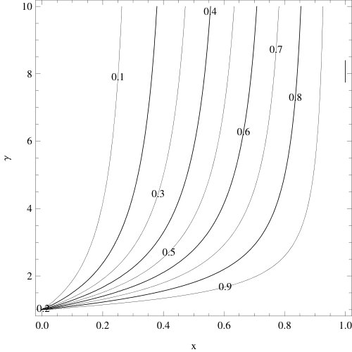 Figure 1
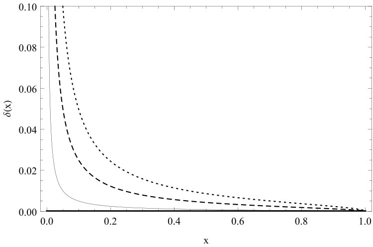 Figure 2
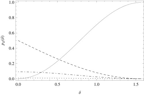 Figure 3
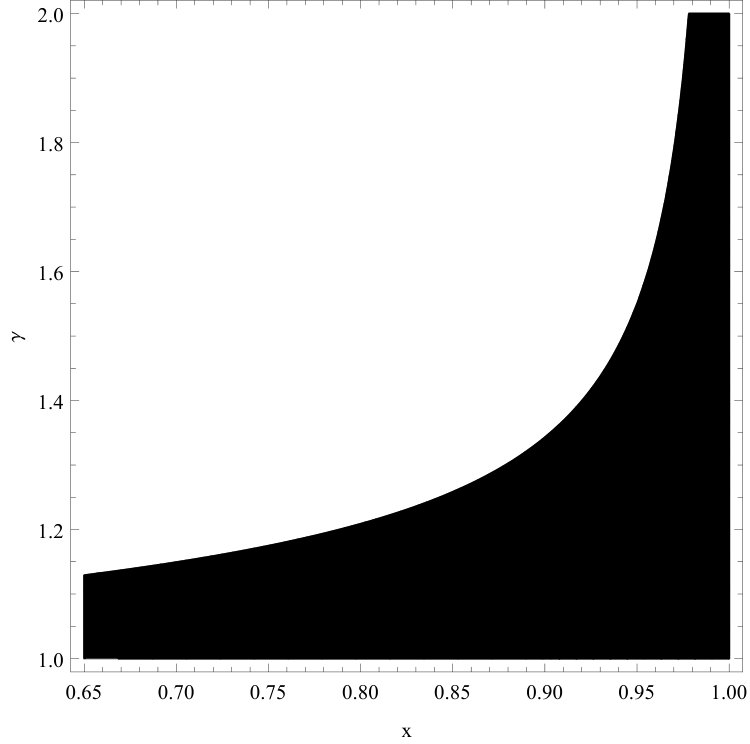 Figure 4
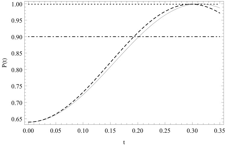 Figure 5
Peer Reviews
No public reviews on file for this paper yet. If you reviewed it on a platform where reviews are public (OpenReview, ICLR, NeurIPS, ICML), you can paste yours below so the community can read it here.
Videos
No videos yet. Explain this paper in a talk, walkthrough, or lecture? Add one.
Theoretical analysis of a nearly optimal analog quantum search
Carlo Cafaro1 and Paul M. Alsing2
1SUNY Polytechnic Institute, 12203 Albany, New York, USA
2Air Force Research Laboratory, Information Directorate, 13441 Rome, New York, USA
Abstract
We analyze the possibility of modifying the original Farhi-Gutmann Hamiltonian algorithm in order to speed up the procedure for producing a suitably distributed unknown normalized quantum mechanical state. Such a modification is feasible provided only a nearly optimal fidelity is sought. We propose to select the lower bounds of the nearly optimal fidelity values such that their deviations from unit fidelity are less than the minimum error probability characterizing the optimum ambiguous discrimination scheme between the two nonorthogonal quantum states yielding the chosen nearly optimal fidelity values. Departing from the working assumptions of perfect state overlap and uniform distribution of the target state on the unit sphere in -dimensional complex Hilbert space, we determine that the modified algorithm can indeed outperform the original analog counterpart of a quantum search algorithm. This performance enhancement occurs in terms of speed for a convenient choice of both the ratio between the energy eigenvalues and of the modified search Hamiltonian and the quantum mechanical overlap between the source and the target states. Finally, we briefly discuss possible analytical improvements of our investigation together with its potential relevance in practical quantum engineering applications.
pacs:
Quantum computation (03.67.Lx), Quantum information (03.67.Ac).
I Introduction
In 1997, Grover presented a quantum algorithm for solving very large database search problems grover97 , one of the outstanding problems in computational science knuth75 . Grover’s search algorithm enables searching for an unknown marked item in an unstructured database of items by accessing the database a minimum number of times. From a classical standpoint, one needs to test items, on average, before identifying the correct item. With Grover’s algorithm however, the same task can be completed successfully with a complexity of order , that is, with a quadratic speed up. The original formulation of Grover’s algorithm was presented in terms of a discrete sequence of unitary logic gates (digital quantum computation). Alternatively, Farhi and Gutmann proposed an analog version of Grover’s algorithm in Ref. farhi98 where the state of the quantum register evolves continuously in time under the action of a suitably chosen driving Hamiltonian (analog quantum computation). For recent discussions on the transition from the digital to analog quantum computational setting for Grover’s algorithm, we refer to Ref. carlo1 ; carlo2 ; cafaro2017 . The formulation of the analog algorithm proposed by Farhi and Gutmann can be briefly described as follows. Consider mutually orthonormal states and assume that only one of them has non-zero energy (energetically marked state). Starting from an equal superposition of the states, the problem is to determine how quickly the system can evolve under a given Hamiltonian so that the energetically marked state is reached with certainty. Within the working assumption of time-independent Hamiltonian evolutions, Farhi and Gutmann showed that their algorithm required a minimum time of the order , thus yielding the same complexity as Grover’s original algorithm. Interestingly, the evolution time for the analog algorithm scaled like , with denoting the energy of the marked state, just as demanded by the time-energy uncertainty principle mandelstam45 . In Refs. mandelstam45 ; vaidman92 ; uffink93 , it was shown that the minimum time interval required for an isolated quantum system to evolve to an orthogonal (that is, perfectly distinguishable) state is inversely proportional to its constant energy spread. Such minimum time is also known as orthogonalization time in the literature. In Ref. margolus98 , the maximum speed of evolution of an isolated quantum system was interpreted in terms of the maximum number of distinct states that the system can explore in a fixed time interval. This fixed time interval was shown to be inversely proportional to the system’s quantum mechanical average energy minus its ground state energy. For a unified tight bound on the rate of quantum dynamical evolution based on both the average energy and the energy spread of the system, we refer to Ref. levitin09 . The presence of a finite non-orthogonality in the context of quantum limits to dynamical evolutions was considered, for instance, in Ref. trifonov99 and Ref. giovannetti03 . In the former work, the expression of the states that minimize the time necessary to evolve, under a time-independent Hamiltonian, from an initial quantum state to a final state that is only approximately orthogonal was found. It is worth noting that the final state is only approximately orthogonal for a given upper bound on the mean energy of a general closed system. In the latter work, on the contrary, an extension of the concept of quantum speed limit to mixed states in the case where the quantum system does not evolve from an initial state to an orthogonal state (that is, the case of non-zero fidelity) was proposed.
In our paper, instead of allowing for a finite non-orthogonality between the quantum states that leads to a non-zero fidelity, we consider a complementary scenario. We allow for a finite non-parallelism that yields a non-unit fidelity. The consideration of nearly optimal state searching is instructive for various reasons. First, it is reasonable to take into account the fact that actual measurements always involve a countable set of outcomes and thus, any realistic measurement device has finite resolution partovi . Second, finite resolution measurements can reveal more about the physical properties of quantum systems than precise measurements furusawa . Third, it is known that a quantum measurement can enhance the transition probability between two pure states fritz10 and, finally, it is indisputable that quantum measurement cannot perfectly discriminate between two nonorthogonal pure states chefles00 .
Motivated by these considerations, the questions we address in this paper can be outlined as follows: First, what is the minimum time necessary to reach a given nearly optimal fidelity value in a continuous time quantum search algorithm? Second, is it possible to formulate a modified version of the original Farhi-Gutmann search algorithm that leads to such a selected fidelity value in a shorter time than the one required by the original Farhi-Gutmann algorithm? Third, how can we reasonably justify the choice of a lower bound for such a nearly optimal fidelity value? We demonstrate that it is possible to extend the original work performed by Farhi and Gutmann in order to speed up the procedure for producing a suitably distributed unknown normalized quantum state with high non-unit fidelity. In particular, by modifying the original working assumptions of perfect state overlap and uniform distribution of the target state on the unit sphere in the -dimensional complex Hilbert space, the newly proposed algorithm can indeed outperform the original analog counterpart of a quantum search algorithm. This is achieved for a convenient choice of both** the ratio ** between the eigenvalues and of the modified search Hamiltonian and the quantum mechanical overlap between the initial and target states.
The layout of the remainder of this paper is as follows. In Section II, we extend the Farhi-Gutmann optimality proof to the case of an imperfect quantum state overlap. In Section III, we present the transition probability for the modified version of the Farhi-Gutmann analog algorithm. In Section IV, we explain how we choose the lower bounds of the nearly optimal fidelity values by means of quantum discrimination techniques. Specifically, we impose that deviations from unit fidelity are less than the minimum error probability characterizing the optimum ambiguous discrimination scheme between the two nonorthogonal quantum states yielding the selected nearly optimal fidelity values. In Section V, we compare in terms of minimum run time the original and the modified quantum search algorithms and identify a two-dimensional parametric region where the modified algorithm outperforms the original one under the working assumption of imperfect state transfer compatible with finite precision quantum measurements. Our concluding remarks appear in Section VI. Finally, technical details on the numerical values of the quantum overlap can be found in Appendix A.
II The modified optimality proof
In this section, we modify the original optimality proof by Farhi and Gutmann in Ref. farhi98 by relaxing the requirement of finding the desired target state with certainty. In particular, we wish to determine how the search time shortens if we only want to achieve a nearly optimal fidelity value.
The optimality proof provided by Farhi and Gutmann in Ref. farhi98 for producing the target state relies on two key working assumptions. First, the target state is produced with absolute certainty. In other words, the modulus squared of the quantum state overlap, that is, the transition probability or transition fidelity at the end of the production procedure is equal to unity. Second, the target state is an unknown element of a given orthonormal basis with of an -dimensional complex Hilbert space with . Our modified optimality proof for an imperfect quantum state overlap follows closely the lines of the original optimality proof presented in Ref. farhi98 . Consider a quantum system, assumed to be initially in a state at time that does not depend on the target state and evolves by means of a Hamiltonian given by,
[TABLE]
where . For the discussion that follows, it is unnecessary to specify the explicit expression for the driving Hamiltonian in Eq. (1). The problem being investigated is that of finding a lower bound on the time for the -independent state to evolve into the state given that its evolution is governed by the time-independent Hamiltonian in Eq. (1). Let us consider the following two initial value problems,
[TABLE]
where denotes the reduced Planck constant. In what follows, we depart from Farhi and Gutmann original optimality proof. We do not require achieving the absolute certainty of producing the target state at the end of the evolution and assume that at time** **we have,
[TABLE]
The normalization condition for** ** requires that the probability amplitudes satisfy the following constraint equation,
[TABLE]
The quantity ** denotes a (normalized) state orthogonal to the target state contained in the two-dimensional subspace of the full Hilbert space spanned by and . A suitable choice for the parametrization of the state **in Eq. (3) is given by,
[TABLE]
where** and are arbitrary real phases while **is assumed to be a small and positive real parameter. Finally, for convenience and without loss of generality, we set so that becomes
[TABLE]
where denotes the complex imaginary unit. In what follows, we assume** so that and . For the sake of clarity, we point out that the validity of this latter working assumption will be explicitly clarified by means of Eq. (38) and Fig. in the next section. **Furthermore, we have
[TABLE]
To find a lower bound on the time , we proceed as follows. First, consider the following quantity
[TABLE]
By using Eqs. (6) and (7) in the expression for appearing in Eq. (8), we obtain after some algebra,
[TABLE]
Substituting Eq. (9) into Eq. (8), we obtain
[TABLE]
Observe that for a set of *complex *amplitude coefficients with , we find
[TABLE]
Therefore, by exploiting Eq. (11), we** **observe that
[TABLE]
By using Eq. (7) in Eq. (12) and neglecting second order terms in we arrive at,
[TABLE]
Observe that for , we have both and . Finally, Eq. (13) reduces to,
[TABLE]
Now, let us consider the following expression,
[TABLE]
After some algebra and exploiting the normalization conditions and , we obtain
[TABLE]
Differentiating with respect to time the LHS (left-hand-side) and the RHS (right-hand-side) of Eq. (16) and recalling that for any where denotes the complex conjugate of , we find
[TABLE]
that is,
[TABLE]
Recalling that and and observing that for any , Eq. (18) becomes
[TABLE]
Employing the Cauchy-Schwarz inequality and recalling that , we obtain
[TABLE]
Summing over the index in Eq. (20), we have
[TABLE]
Since and , and using Eq. (11), the RHS in the inequality written in Eq. (21) becomes
[TABLE]
Combining Eqs. (21) and (22), we obtain
[TABLE]
Integrating Eq. (23) with respect to time and recalling the initial conditions , we find
[TABLE]
Finally, by combining Eq. (14) and Eq. (24) evaluated at , we have
[TABLE]
that is,
[TABLE]
or, equivalently,
[TABLE]
Equation (27) is our first finding reported in this paper and can be regarded as the analog of Eq. (23) in Ref. trifonov99 obtained in the context of finding states that minimize the evolution time to become an almost orthogonal state. We point out that although it is expected that** ,** the scaling behavior of** as a function of the angle with is not at all obvious. We emphasize that the validity of Eq. (27) is limited to the case in which the target state is an unknown element of a given orthonormal basis with of an -dimensional complex Hilbert space. We also recall that is defined by the relation with **. The unitary operator is the usual quantum mechanical evolution operator. Therefore in general, the quantity can depend on certain characteristics of the chosen time-independent search Hamiltonian .
For the sake of clarity, we point out that our proposed modified optimality proof is not meant to be used to determine the optimality of a modified continuous time quantum search algorithm. The lower bound in Eq. (27) is only** **useful for providing the optimality of the scaling of the complexity of any algorithm specified by the Hamiltonian in Eq. (1). In particular, its purpose is to find out the behavior with respect to the parameter of the minimum time necessary to achieve a desired nearly optimal transition probability value (that is, with ) when evolving from a source state to an approximate target state under the Hamiltonian in Eq. (1). In other words, we have not compared the optimality of two distinct algorithms that aim to solve the same identical task. Instead, we are interested in finding out how the performance of a single algorithm, quantified in terms of the minimum time necessary to accomplish the task, is affected when two distinct tasks have to be completed. In our case, the first task (that is, the original task) is to find the target state with certainty (that is, success probability equal to one). The second task (that is, the modified task), instead, is to search for an approximate target state that corresponds to a success probability that is only nearly equal to one. In summary, when considering the original task, we go from to with success probability one and . In the modified task, we go from to with success probability where and . In both cases, the same algorithm described by the Hamiltonian in Eq. (1) is employed.
Our proposed modified optimality proof allowed us to formally introduce the parameter in a general physical setting where it is not necessary to specify the explicit expression of the driving Hamiltonian in Eq. (1). The following section, instead, includes a more specific discussion on the functional form of the parameter for a specific choice of the driving Hamiltonian.
III The modified Farhi-Gutmann search Hamiltonian
In this section, we present the transition probability for the modified version of the Farhi-Gutmann analog search algorithm. Assume that the time-independent Hamiltonian in Eq. (1) is given by,
[TABLE]
where,
[TABLE]
Observe that when , the Hamiltonian reduces to the Hamiltonian as originally proposed by Farhi and Gutmann in Ref. farhi98 . Furthermore, assume that is the normalized target state while is the normalized initial state with that evolves in an unitary fashion according to Schrödinger’s quantum mechanical evolution law,
[TABLE]
where the time-independent Hamiltonian is given in Eq. (28). We wish to compute the time such that the transition probability defined as,
[TABLE]
assumes its maximum value** . Introducing the orthonormal basis ** with and , after some straightforward but tedious matrix algebra computations, the explicit expression** of **in Eq. (31) becomes
[TABLE]
where in Eq. (32). Observe that for , we recover from the expression of in Eq. (32) the original fidelity expression as obtained by Farhi and Gutmann in Ref. farhi98 ,
[TABLE]
To find the instant for which , we proceed as follows. First, from Eq. (32), we observe that equals
[TABLE]
In Fig. , we present the contour plot that exhibits v.s. with and . In particular, the level curves are defined by the relation (with in Eq. (48)) where is a constant with numerical values such that . As a side remark, notice that when , that is , for any value of in agreement with what was** **reported in Ref. farhi98 . Second, the instant for which with and in Eqs. (32) and (34), respectively, satisfies the relation
[TABLE]
that is, since ,
[TABLE]
Once again, observe that in the limiting case of , we recover the original relation found in Ref. farhi98 ,
[TABLE]
We recall that at the end of Section II, we stated that the quantity can depend on specific properties of the Hamiltonian ** **in Eq. (28). By using Eqs. (3) and (34), we can finally obtain the explicit functional form of in terms of the two parameters and ,
[TABLE]
Using Eq. (38), we present in Fig. 2 a plot of versus for a number of fixed values of greater than one. Finally, observe that for , for any choice of and we recover the limiting case discussed in Ref. farhi98 .
IV Lower bounds on the fidelity values
Having introduced the parameter in a general setting in Section II (see Eq. (27)) and in a more specific framework in Section III (see Eq. (38)), we would like to address in Section IV the following question: How big can be chosen? In principle, we could arbitrarily choose a nearly optimal threshold value of the error probability for quantum search. However, in what follows, we propose a way to justify to a certain extent this arbitrariness with some plausible line of reasoning. First, at the end of the search, we expect that the approximate and the exact target states will be very close. Therefore, the error probability for quantum search (that is, its deviation from the unit fidelity) will be very small. Second, since these target states have a large overlap, it will be difficult to distinguish them. Therefore, we also expect that the error probability for quantum state discrimination will be large. Given these two considerations, it is intuitive that in our working conditions the error probability for quantum search will be smaller than the error probability for quantum state discrimination. However, even in the presence of large overlaps between quantum states, it is possible to device highly successful quantum state discrimination protocols where the minimum error probability can be made arbitrarily small. We propose to select the minimum success probability values for quantum search by imposing that the deviation from the unit fidelity is smaller than the smallest (compatible with realistic finite-precision quantum measurements) minimum error probability achievable in highly successful quantum state discrimination protocols for quantum states with very large overlaps.
If we desire to consider a very small departure** **from the unit fidelity,
[TABLE]
we expect** ** with , that is
[TABLE]
Therefore, the question becomes: How small should the** real parameter in Eq. (40) be chosen? How do we select this value? Can we physically motivate such a choice for ? In what follows, motivated by theoretical quantum state discrimination principles chefles00 ; croke09 and acknowledging the presence of imperfections in actual quantum measurement settings that limit the precision of the measurement of angles gisin12 ; mario18 , we propose a way to select the numerical upper (lower) bounds for (). **
We recall that the goal in a quantum state discrimination problem is to identify the actual state of a quantum system that is prepared, with a fixed prior probability, in a specific but unknown state that belongs to a finite set of given possible states chefles00 ; croke09 . An essential property of quantum mechanics is that two pure states cannot be distinguished perfectly, if they are not orthogonal. Therefore, there are fundamental limitations in quantum state discrimination protocols on the success with which one can determine the actual state. Specifically, when the possible states are not mutually orthogonal, it is not possible to develop a state-distinguishing protocol that can discriminate between them perfectly. Relevant state-distinguishing techniques are the unambiguous ivanovic87 ; dieks88 ; peres88 and the ambiguous holevo73 ; yuen75 ; helstrom76 state discrimination schemes. Unambiguous state discrimination requires that, whenever a definite (that is, conclusive) outcome is recorded after the measurement, the result must be error free (that is, unambiguous). When the measurement fails to provide a definite outcome, a nonzero probability of inconclusive outcomes has to be taken into consideration. Then, the optimum unambiguous discrimination scheme is realized when the failure probability (that is, the probability of inconclusive outcomes) is minimum. On the contrary, ambiguous state discrimination requires that a conclusive outcome has to be recorded in each single measurement. This in turn implies that the discrimination is ambiguous since errors in the conclusive result are unavoidable. Based on the measurement outcome, a guess is made as to what the actual state of the quantum system was. Then, the optimum ambiguous discrimination scheme is obtained when the error probability (that is, the probability of making a wrong guess) is minimum. For a very instructive discussion on how to interpret the original Farhi-Gutmann analog quantum search algorithm as a method for improving the distinguishability of a set of Hamiltonians by adding a controlled driving term, we refer to Ref. childs00 .
Being in the framework of ambiguous quantum state discrimination, assume that we are given one of two normalized quantum states and , not necessarily orthogonal, with prior probabilities and , respectively. Furthermore, assume we have been asked to optimally determine which state we have actually been given. It happens that the** **minimum error probability is given by chefles00 ; croke09 ,
[TABLE]
From Eq. (41), we note that the minimum error probability is a monotonic increasing function of the quantum mechanical overlap . In particular, when approaches zero (that is, very large quantum overlap) and , it can become quite challenging to distinguish the state from the state since the probability of making an incorrect guess approaches .** Alternatively, we point out that in the presence of large asymmetry between the prior probabilities and , the success of the discrimination protocol increases and, as a consequence, it becomes less difficult to discriminate between and . For instance, when , the minimum error probability approaches the liming value as the angle approaches zero. We observe that the quantum mechanical overlap plays a key role in both quantum state discrimination and nearly optimal analog quantum search. In the former case, it is the essential quantity that sets a bound to the effectiveness of the discrimination scheme. In the latter case, it quantifies the departure from the perfect unit fidelity. **In view of the above mentioned considerations, it becomes useful to define an approximate target state as a quantum state with a nearly optimal fidelity that departs from the unit perfect fidelity by an amount . We impose that the quantity is smaller than the minimum error probability in Eq. (41),
[TABLE]
Eq. (42) implies that we choose to select the lower bounds of the nearly optimal fidelity values in such a manner that their deviations from the unit fidelity are less than the minimum error probability characterizing the optimum ambiguous discrimination scheme between the two nonorthogonal quantum states (that is, the approximate and the exact target states, respectively) yielding the chosen nearly optimal fidelity values. A plot of as a function of the angle for a variety of sets of a priori probabilities appears in Fig.** . We point out that the proposed inequality in Eq. (42) is reminiscent of the (sandwich) Fuchs-van de Graaf inequalities relating the trace norm distance and the fidelity as suitable measures of closeness for quantum states fuchs99 . Indeed, the trace norm distance appears in the expression for the minimum error probability while the fidelity appears in the equation for the transition probability in our discussion. For the sake of completeness, we also remark that while Fuchs and van de Graaf were only concerned with the problem of distinguishing between two quantum states with equal a priori probabilities, an extension of their analysis to the case of arbitrary a priori probabilities can be found in Ref. mr14 . As a final consideration, we emphasize that in the limiting case of equal a priori probabilities together with the conditions , **it is straightforward to verify that our inequality in Eq. (42) can be obtained from the Fuchs-van de Graaf inequalities. In particular, as explained below, the sharpness of the bounds that we propose in Eq. (42) can be tuned by means of the degree of asymmetry that specifies the a priori probabilities of the two quantum states being distinguished.
Recalling Eq. (40), the problem was the determination of how small the real parameter in Eq. (40) should be. We are now in the condition to provide an answer to this issue. We note that, after some straightforward algebra and using Eq. (39), the inequality constraint in Eq. (42) yields
[TABLE]
The quantity in Eq. (43) denotes a fixed value of the prior probability . Knowing that and setting with being the degree of asymmetry between the two *a priori *probabilities and , Eq. (43) becomes
[TABLE]
We observe that in the maximally symmetric scenario, we have (that is, ). Instead, in the maximally asymmetric scenario, we have (that is, ) or (that is, ). Equating Eqs. (40) and (44), we obtain a formal expression for in terms of the degree of asymmetry coefficient ,
[TABLE]
From Eq. (45), we note that to get an of the order of , one needs to have of the order of .** **As previously mentioned, highly successful discrimination protocols characterized by very small minimum error probability values can be obtained when strong asymmetries between the prior probabilities and occur. In such cases, the values of can be rather small. For instance, when , and . We point out that this order of magnitude of angles is quite small. Indeed, in real world settings one necessarily deals with imperfect measurements where intrinsic uncertainties yielding non-negligible systematic errors may be present. For instance, the intrinsic uncertainty of a polarization rotor, typically of the order of on the Bloch sphere (where rad.), limits the precision of the measurement on a polarization qubit gisin12 .
For the sake of clarity, we point out that in our numerical calculations that appear into the next section, the two a priori** probabilities and will not be arbitrarily chosen. They will be chosen in such a manner to yield highly successful discrimination protocols in which it is not difficult to discriminate between the exact and approximate quantum states despite their high degree of overlap. Such protocols are characterized by very low minimum error probability, which, in turn, is achievable when there is a sufficient degree of asymmetry between the two a priori probabilities corresponding to the two states that we wish to distinguish (see Fig. ). Then, to a larger there corresponds a smaller . Specifically, we shall be considering asymmetries of the order of since they yield minimum error probability values of the order of which are low enough for high degree of overlaps specified by angles of the order of rad. Then, being in the framework of highly successful quantum discrimination protocols, we choose the accuracy the search has to achieve by imposing that the departure of the unit fidelity from the nearly optimal desired fidelity value ** must be smaller than the already small minimum error probability . Imposing that is of the order of the maximum achievable angular resolution in a typical quantum mechanical experiment gisin12 , we find how asymmetric the two a priori probabilities must be chosen in order to guarantee the required accuracy the search should achieve.
In what follows, we compare the performances of the original and the modified Farhi-Gutmann analog quantum search algorithms. Clearly, both algorithms are stopped when they reach the same chosen lower bound.
V Comparison of the two search algorithms
In this section, we identify a two-dimensional parametric region where the original algorithm is outperformed by the modified one provided one focuses on nearly optimal fidelity values compatible with the maximum resolution of the previously mentioned quantum discrimination protocol. For the sake of convenience, we shall refer to the original Farhi-Gutmann algorithm () as the special algorithm while the general algorithm denotes the modified version of the Farhi-Gutmann algorithm where with . The transition probability with obtained for the general scenario in Eq. (32) is** **denoted as,
[TABLE]
The maximum value of in Eq. (46) is obtained at the time ,
[TABLE]
and, furthermore,
[TABLE]
Setting , we recover the main findings of Farhi and Gutmann. Specifically, the transition probability in Eq. (46) reduces to in Eq. (33). The maximum value of is obtained at the time ,
[TABLE]
and, furthermore,
[TABLE]
We propose to rank the performance of the two algorithms in two different ways given that Eq. (42) is satisfied: i) rank the two algorithms by comparing the two transitions probabilities evaluated at an identical fixed-value of the travel time; ii) rank the two algorithms by comparing the two minimum travel times needed to arrive at an identical fixed-value of the transition probability.
In the first scenario, since , we wish to determine whether or not there is, for a fixed value of less than , a two-dimensional parametric region ,
[TABLE]
where the general algorithm outperforms the special algorithm in terms of transition probability values in the working assumption of accepting transition probability values less than one.
In the second scenario, since , we wish to determine whether or not there is, for a fixed value of less than one, a two-dimensional parametric region ,
[TABLE]
where the general algorithm outperforms the special algorithm in terms of minimum travel times at fixed** **nearly optimal transition probability values.
Note that in Eq. (52) is such that,
[TABLE]
where, after some algebraic manipulations, we find
[TABLE]
We emphasize that both two-dimensional parametric regions and in Eqs. (51) and (52), respectively, are non-empty sets and in addition, it can be numerically verified that they are identical. Moreover, for the sake of completeness we also point out that one can investigate whether or not the general algorithm outperforms the special one for a given transition probability threshold given that Eq. (42) is satisfied. For this reason, we consider the following sub-region of in Eq. (52),
[TABLE]
A plot of the two-dimensional parametric region in Eq. (55) where the general algorithm outperforms the special algorithm when assuming and appears in Fig**.** .
Finally, for the sake of clarity, we also present in Table I illustrative numerical estimates of in Eq. (47) and in Eq. (54) for a number of selected values of the threshold probability in Eq. (48) under the working assumptions that and . Given the chosen values of the angle in Table I, the numerical estimates of the minimum error probability are calculated by assuming which yields a maximum value of that equals .
As a further clarifying remark, we point out that the numerical values (originated from our proposed comparison of the two algorithms and reported in Table I) were computed by considering the minimum time such that the desired success probability values were obtained. We have simply chosen the desired success probability values to be equal to the maximal success probability values of the modified algorithm in our analysis. However, as evident from Fig.** , we could have chosen different threshold values (leading to shorter minimum times) and still outperform the original algorithm (provided that only a nearly optimal search is considered). As a side remark, we emphasize that this line of reasoning extends naturally to any desired success probability value taken as the maximal success probability with ** in Eq. (48) and where the points** can be chosen to belong to the black-colored region in Fig. . Specifically, in Fig. ** we plot (dashed line) and** (solid line) as a function of time . For the sake of reasoning, we set , , , and . The two horizontal lines in Fig. denote two selected success probability values, (dotted line) and (dotted-dashed line). The threshold value was taken from the fourth line in Table I. We note that the minimum time such that the two desired success probability values are obtained is smaller in the case of the modified algorithm for both selected thresholds. Specifically, in the first and second scenarios, we have and ,** respectively. Note that in the MKSA unit system,** . Since we have considered in our numerical computations, time **is assumed to be dimensionless.
Finally, for a more detailed discussion on the probability of small and large numerical values of the quantum overlap , we refer to Appendix A.
VI Concluding Remarks
In this paper, we focused on the problem of nearly optimal state searching and we demonstrated that it is possible to modify the original Farhi-Gutmann search Hamiltonian (see Eq. (28)) in order to speed up the procedure for finding a suitably distributed unknown normalized quantum state under the working assumption that only a nearly optimal fidelity is achieved,
[TABLE]
with** where and denote the exact and the approximate target states, respectively. More specifically, upon relaxing the working assumptions of exact state overlap and uniform distribution of the target state on the unit sphere in the -dimensional complex Hilbert space, we showed that the proposed algorithm (see Eq. (28)) can indeed outperform the original analog counterpart of a quantum search algorithm. This enhanced **performance occurs for a convenient choice of both the ratio between the eigenvalues of the modified search Hamiltonian and the quantum mechanical overlap between the initial and the target states.
In summary, the main results of our work can be described as follows. First, we extended the optimality proof presented in Ref. farhi98 to the case of nearly optimal state searching and determined that the minimum time interval to find the target state with probability is given by (see Eq. (27)),
[TABLE]
Second, we computed the transition probability (see Eq. (32)) that arises from our proposed search algorithm and determined its maximum value (see Eq. (34) and Fig. ) together with the instant (see Eq. (36)) at** **which this maximum is achieved. Third, from the formal introduction of the quantity in Eq. (3) and the expression of in Eq. (34), we found an explicit expression for the quantity (see Eq. (38) and Fig. ) responsible for our imperfect state search in terms of the two parameters and that characterize our search Hamiltonian,
[TABLE]
Fourth, we introduced the notion of approximate target state . Such a quantum state is characterized by a sufficiently large overlap with the exact target state so that, as we proposed, the deviation from the unit fidelity is smaller than the minimum error probability achievable in an optimal quantum state discrimination protocol (see Fig. ) for the set of quantum states ,
[TABLE]
with defined in Eq. (41). Finally, using numerical methods, we showed that for a fixed transition probability threshold and suitably chosen non-uniform probability distribution functions of the target state on the unit sphere (see Eq. (63)), there exist two-dimensional parametric regions (see Eq. (55)) in which the proposed algorithm outperforms the original one in terms of speed (see Fig. , Table I, and Fig. ) for the special task (namely, finding the approximate target state) it sets out to solve.
We believe that our analysis presented in this paper can serve as a relevant starting point for a more rigorous investigation that would include both theoretical and experimental aspects of the tradeoff between fidelity and run time of quantum search algorithms. For instance, it is known that to mitigate the effect of decoherence originating from the interaction of a quantum system with the environment, it is helpful to decrease the control time of the control fields employed to generate a target quantum state or a target quantum gate. Simultaneously, to enhance the fidelity of generating such targets and reach values arbitrarily close to the maximum , it may be convenient to increase the control time beyond a certain critical value. When the control time reaches a certain value that may be close to the just mentioned critical value however, decoherence can become a dominant effect. Therefore, investigating the tradeoff between fidelity and time control can be of great practical importance in quantum computing rabitz12 ; rabitz15 ; cappellaro18 . For instance, one can design algorithms seeking suboptimal control solutions for much reduced computational effort, since it is very challenging to find a rigorous optimal time control and in many cases the control is only required to be sufficiently precise and short. For example, the fidelity of tomography experiments is rarely above due to the limited control precision of the tomographic experimental techniques as pointed out in Ref. rabitz15 . Under such conditions, it is unnecessary to prolong the control time since the departure from the optimal scenario is essentially negligible. Hence, it can certainly prove worthwhile to design slightly suboptimal algorithms that can be much cheaper computationally. Our analysis can be improved in a number of ways. First, our work can be strengthened by explicitly considering the quantum measurement process in our analysis. For instance, it is known that quantum measurement can be regarded as a decoherence process that potentially enhance or reduce a transition probability between two quantum states fritz10 . Second, as a starting point of our investigation, we could consider a more general time-independent search Hamiltonian where the probability of obtaining the target state can be very large and nearly one kwon02 . Furthermore, in order to work in a more realistic setting, nearly optimal time-dependent search Hamiltonians specified in terms of the so-called schedule function of the search algorithm could also be considered chuang17 . Finally, from a more ambitious perspective, we could explore the manner in which recent investigations on intelligent forms of quantum searching algorithms in the presence of imperfections, with the help of techniques borrowed from quantum machine learning lloyd17 , would connect to our nearly optimal quantum search problem.
In conclusion,** **we hope to pursue a more rigorous and realistic analysis that includes these intriguing theoretical and experimental aspects in forthcoming scientific efforts.
Acknowledgements.
C. C. is grateful to the United States Air Force Research Laboratory (AFRL) Summer Faculty Fellowship Program for providing support for this work. Any opinions, findings and conclusions or recommendations expressed in this paper are those of the authors and do not necessarily reflect the views of AFRL. Finally, constructive criticism from two anonymous referees leading to an improved version of this manuscript are sincerely acknowledged by the authors.
Appendix A Numerical values of the quantum overlap
In this Appendix, we present a more in depth discussion on the probability of small and large numerical values of the quantum overlap .
In general, one may argue that large values of the overlap are not very typical or particularly realistic since they occur when the source state is essentially already the desired target state. This objection has its merit when one assumes that the realistic scenario is the one in which no a priori information on the target state is available and, in particular, the target state is assumed to be a normalized vector in a list of possible orthonormal states. Indeed, within these working assumptions, and the largest value of that would be considered realistic is obtained for and equals . However, one can envision a circumstance in which *a priori relevant *knowledge is available so that the target state is a suitably chosen non-uniformly distributed normalized vector in a -dimensional vector space. In such a scenario, the probability of occurrence of large values of can begin to be non-negligible. Thus, large values of can become realistic in these new working conditions. We point out that *a priori *knowledge happens to be useful in both quantum metrology and imperfect (optimal) quantum cloning. In the former case, in order to design the best parameter estimation scheme, some form of a priori knowledge of such a parameter is required paris18 . In the latter case, instead, knowledge of the distribution of qubits on the Bloch sphere that encodes some a priori information on a given quantum state that one desires to clone is taken advantage of in order to achieve the highest fidelity karol10 ; kang16 . For instance, in the specific framework of phase-independent quantum cloning, one assumes to clone qubits that are a priori known to be symmetrically distributed around the Bloch vector karol10 .
As pointed out in Section II, the optimality proof by Farhi and Gutmann occurs under the special working assumption that the target state is an unknown element of a given orthonormal basis with of an -dimensional complex Hilbert space with . As pointed out earlier, in this scenario it is rather unlikely that assumes values close to one. In their more general setting however, Farhi and Gutmann assume that the target state is an arbitrary normalized vector in a -dimensional complex Hilbert space which is uniformly distributed on the unit sphere farhi98 .
We briefly recall that the space enclosed by a -dimensional unit sphere is a -ball whose infinitesimal volume element in spherical coordinates is given by,
[TABLE]
where for any and . Furthermore, the volume element of the -dimensional unit sphere generalizes the concept of the area element of a two-dimensional unit sphere and, from Eq. (60), is given by
[TABLE]
Returning to our discussion, we assume that the probability density function that describes the distribution of the states on the -dimensional unit sphere depends on the coordinate , denoted as , which is uniform with respect to the remaining coordinates. Therefore, by** **marginalizing over all the unimportant integration variables but with where , we find that the probability that is greater than a given value is given by farhi98 ,
[TABLE]
The quantity in Eq. (62) denotes a well-defined probability density function (pdf), that is to say, a pdf that is positive and normalized to one. For the sake of reasoning, we select to be at the north pole. Generalizations to less peculiar scenarios are straightforward. In what follows, we provide some rationale for our choice of . The functional form of is essentially that of a Gaussian with mean and variance multiplied by a suitably chosen oscillatory function. The mean is set equal zero, while any value of between [math] and can be chosen provided that the variance is not too small. Furthermore, the multiplying factor in the proposed expression of is chosen in such a manner as** **to substantially mitigate the oscillatory behavior of in Eq. (62) and leads when multiplied with it, to an approximately constant function over the selected domain of integration. Practically, one can consider a narrowly distributed Gaussian peaked nearby the location of the initial state or, for a Gaussian peaked far away from such a location, the width of the Gaussian has to be suitably larger. Under this assumption, a convenient choice for our analysis is given by the following pdf,
[TABLE]
In Eq. (63), is a normalization factor that depends on the choice of and . For instance, for , , and , by means of numerical integration, we find Prob. We note that with a smaller , the probability of being greater than a selected value increases and asymptotically approaches unity. For instance, for and , we observe that Prob and Prob, respectively. We point out that if and is uniform as selected in Ref. farhi98 , Prob. Therefore, although the probability is not exactly zero, it is very unlikely that is close to when assuming uniformity for . For this reason, we considered here nearly optimal (imperfect) state searches where the target state is not uniformly distributed on the unit sphere. As a final remark, we point out that the assumption that the target state is selected at random means that we assume absolute ignorance (that is, maximum entropy) about the location of the target. If we somehow learn an important piece of information about the location of the target however, one can think of updating his/her state of knowledge (see Ref. cafaropre , for instance) about the target with a new probability density function of the state on the -dimensional space. As a consequence, the search algorithm can be adapted to the target in order to improve the efficiency of the searching scheme. We emphasize that these considerations are reminiscent of what happens in channel-adapted quantum error correction cafaro14 ; fletcher07 ; cafaroosid and adaptive quantum computing briegel15 where classical learning techniques can be used to enhance the performance of certain quantum tasks briegel16 . We leave the exploration of these intriguing ideas to future investigations.
The reference list from the paper itself. Each links out to its DOI / PubMed record.
- 1(1) L. K. Grover, Quantum mechanics helps in searching for a needle in a haystack , Phys. Rev. Lett. 79 , 325 (1997).
- 2(2) D. E. Knuth, The Art of Computer Programming, Vol. 3 : Sorting and Searching , Addison-Wesley, Reading, MA (1975).
- 3(3) E. Farhi and S. Gutmann, Analog analogue of a digital quantum computation , Phys. Rev. A 57 , 2403 (1998).
- 4(4) C. Cafaro and S. Mancini, An information geometric viewpoint of algorithms in quantum computing , in Bayesian Inference and Maximum Entropy Methods in Science and Engineering, AIP Conf. Proc. 1443 , 374 (2012).
- 5(5) C. Cafaro and S. Mancini, On Grover’s search algorithm from a quantum information geometry viewpoint , Physica A 391 , 1610 (2012).
- 6(6) C. Cafaro, Geometric algebra and information geometry for quantum computational software , Physica A 470 , 154 (2017).
- 7(7) L. Mandelstam and I. Tamm, The uncertainty relation between energy and time in non-relativistic quantum mechanics , J. Phys. USSR 9 , 249 (1945).
- 8(8) L. Vaidman, Minimum time for the evolution to an orthogonal quantum state , Am. J. Phys. 60 , 182 (1992).