Towards a more complex description of chemical profiles in exoplanets retrievals: A 2-layer parameterisation
Quentin Changeat, Billy Edwards, Ingo Waldmann, Giovanna Tinetti

TL;DR
This paper introduces a 2-layer parameterisation for exoplanet atmospheric retrievals, allowing pressure-dependent chemical profiles to be inferred from spectra, which enhances the interpretation of future high-quality observations.
Contribution
It presents a novel 2-layer retrieval method that captures vertical chemical discontinuities without relying on prior models, improving atmospheric characterization accuracy.
Findings
The 2-layer model accurately retrieves chemical profile discontinuities.
Assumptions on chemical profiles significantly affect atmospheric parameter estimates.
Future spectra can constrain pressure-dependent chemical variations.
Abstract
State of the art spectral retrieval models of exoplanet atmospheres assume constant chemical profiles with altitude. This assumption is justified by the information content of current datasets which do not allow, in most cases, for the molecular abundances as a function of pressure to be constrained. In the context of the next generation of telescopes, a more accurate description of chemical profiles may become crucial to interpret observations and gain new insights into atmospheric physics. We explore here the possibility of retrieving pressure-dependent chemical profiles from transit spectra, without injecting any priors from theoretical chemical models in our retrievals. The "2-layer" parameterisation presented here allows for the independent extraction of molecular abundances above and below a certain atmospheric pressure. By simulating various cases, we demonstrate that this…
Click any figure to enlarge with its caption.
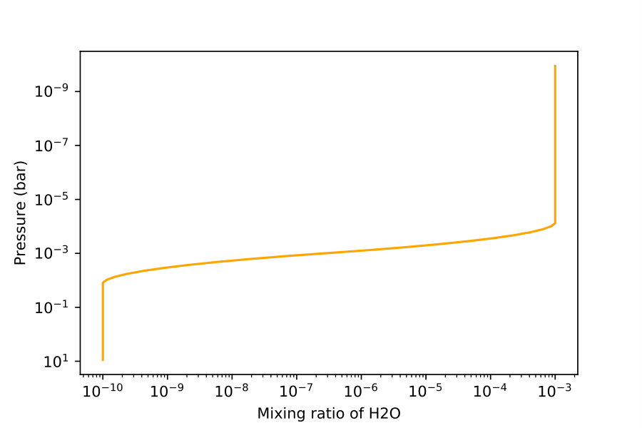 Figure 1
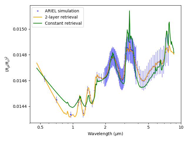 Figure 2
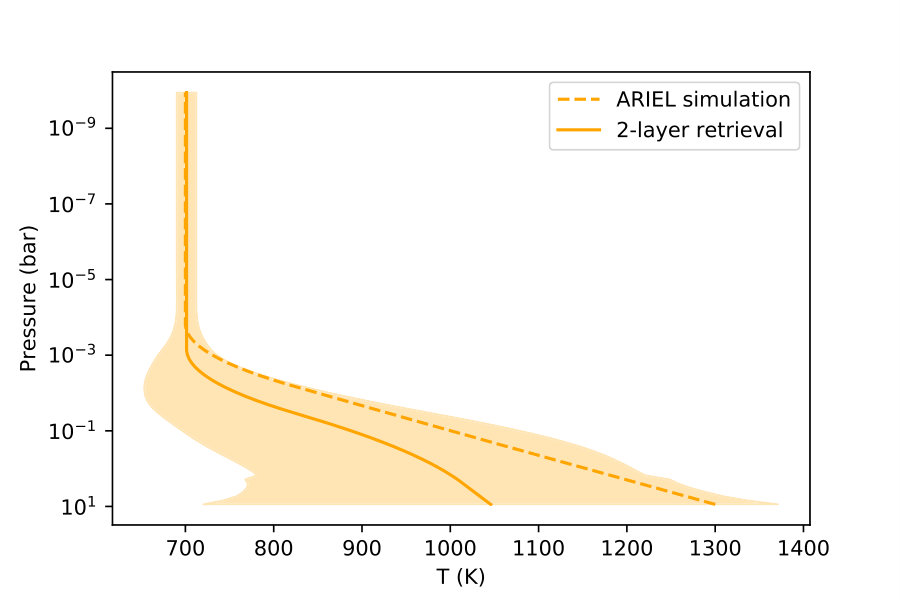 Figure 3
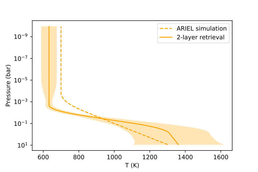 Figure 4
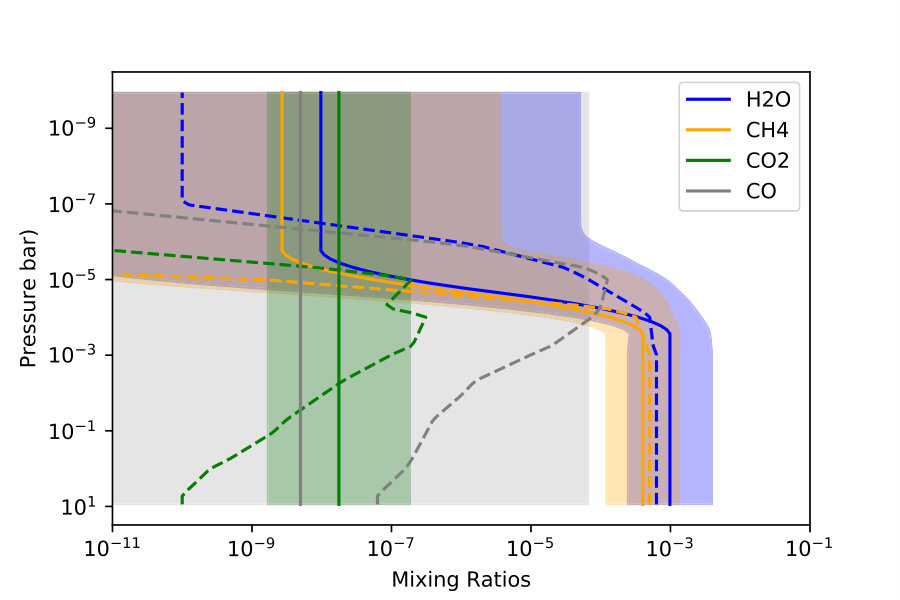 Figure 5
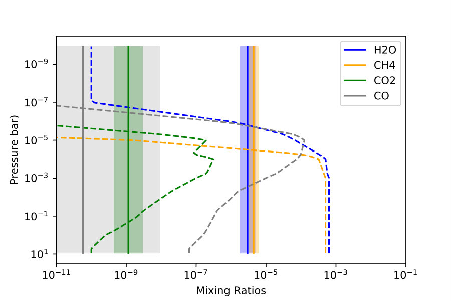 Figure 6
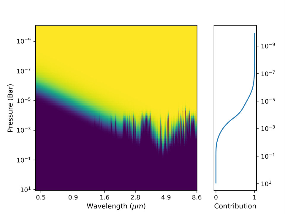 Figure 7
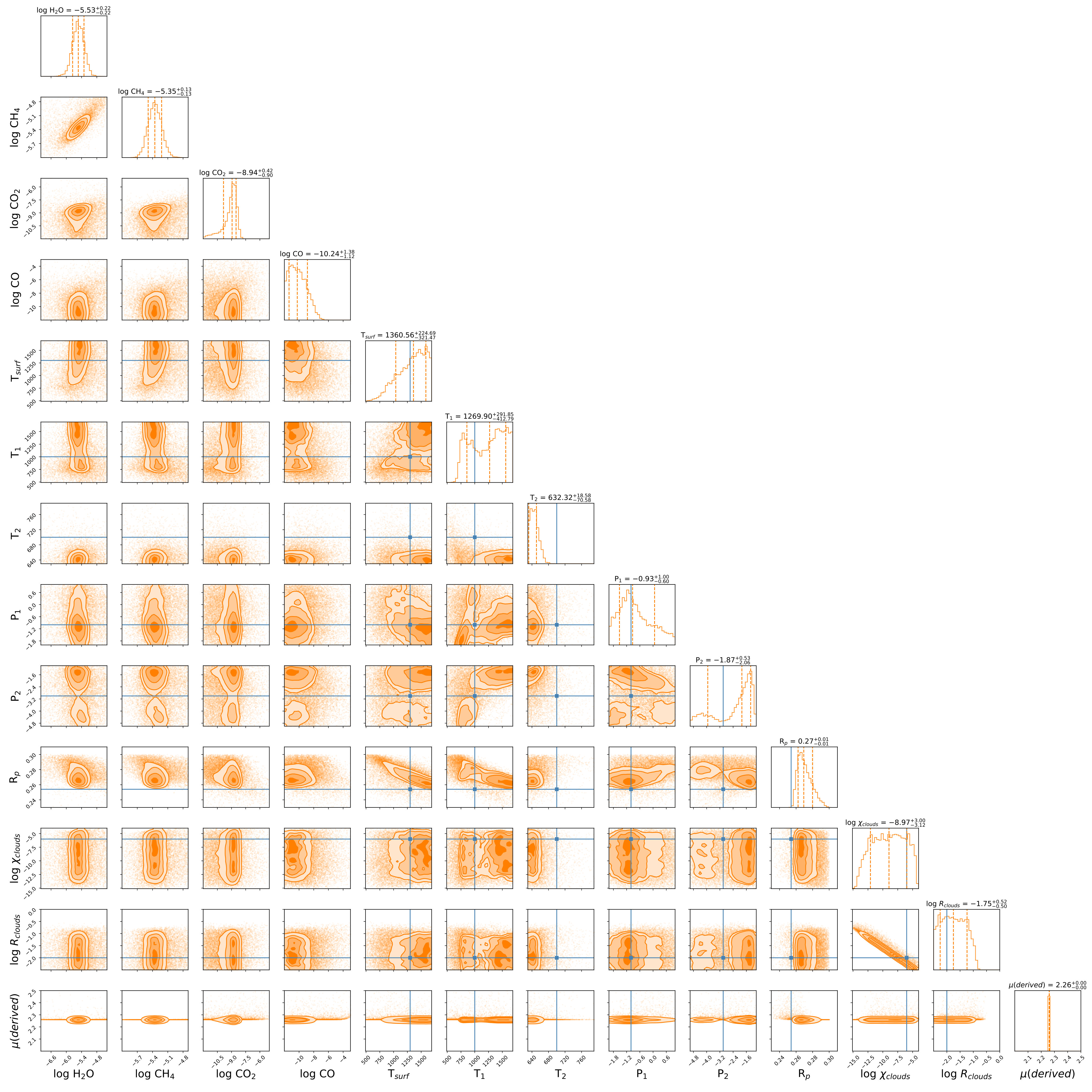 Figure 8
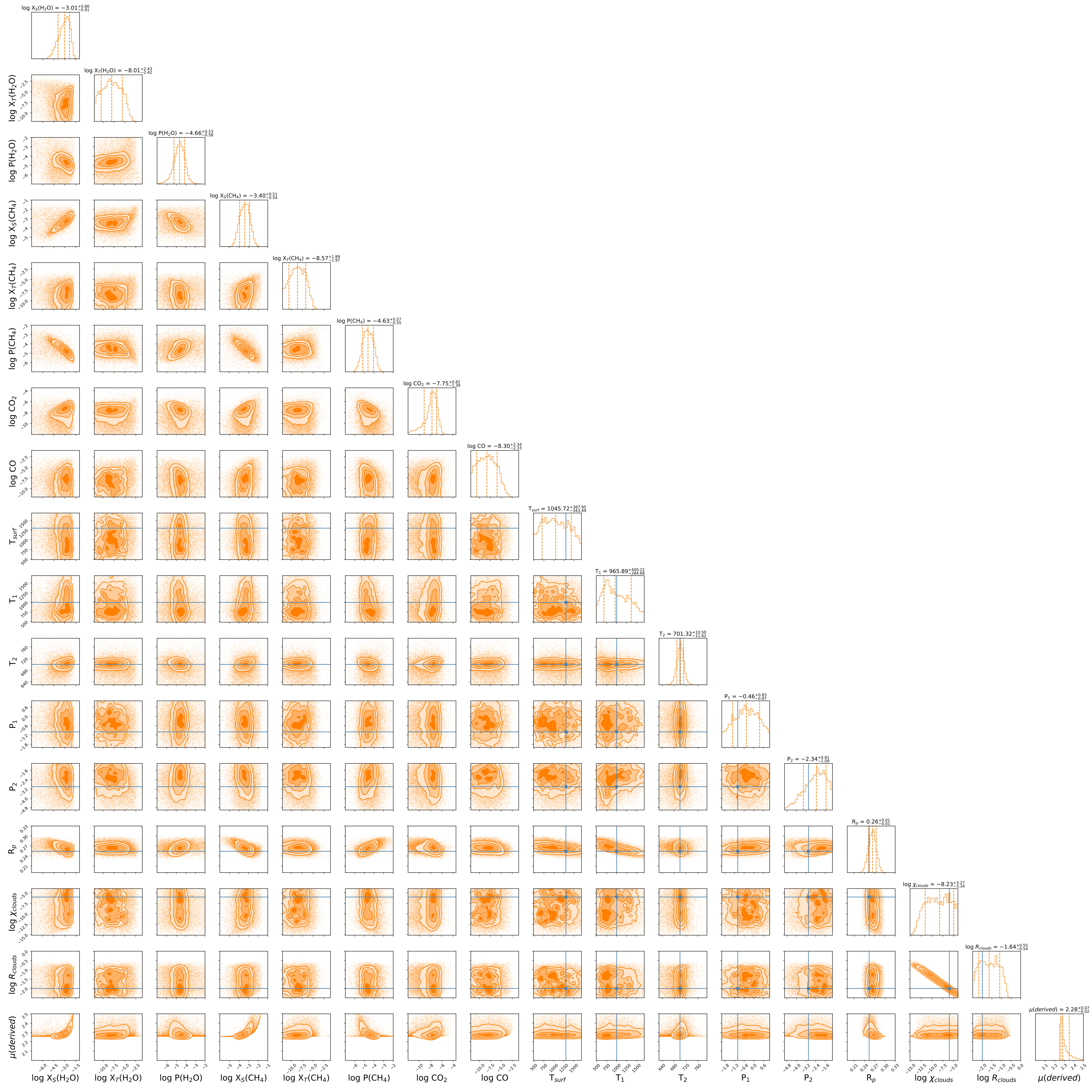 Figure 9
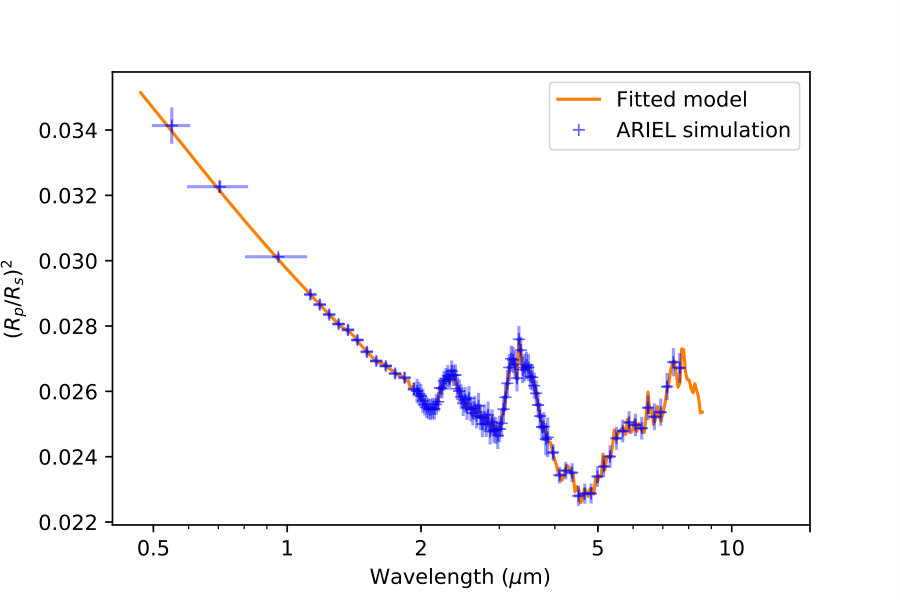 Figure 10
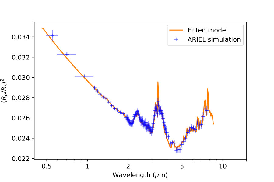 Figure 11
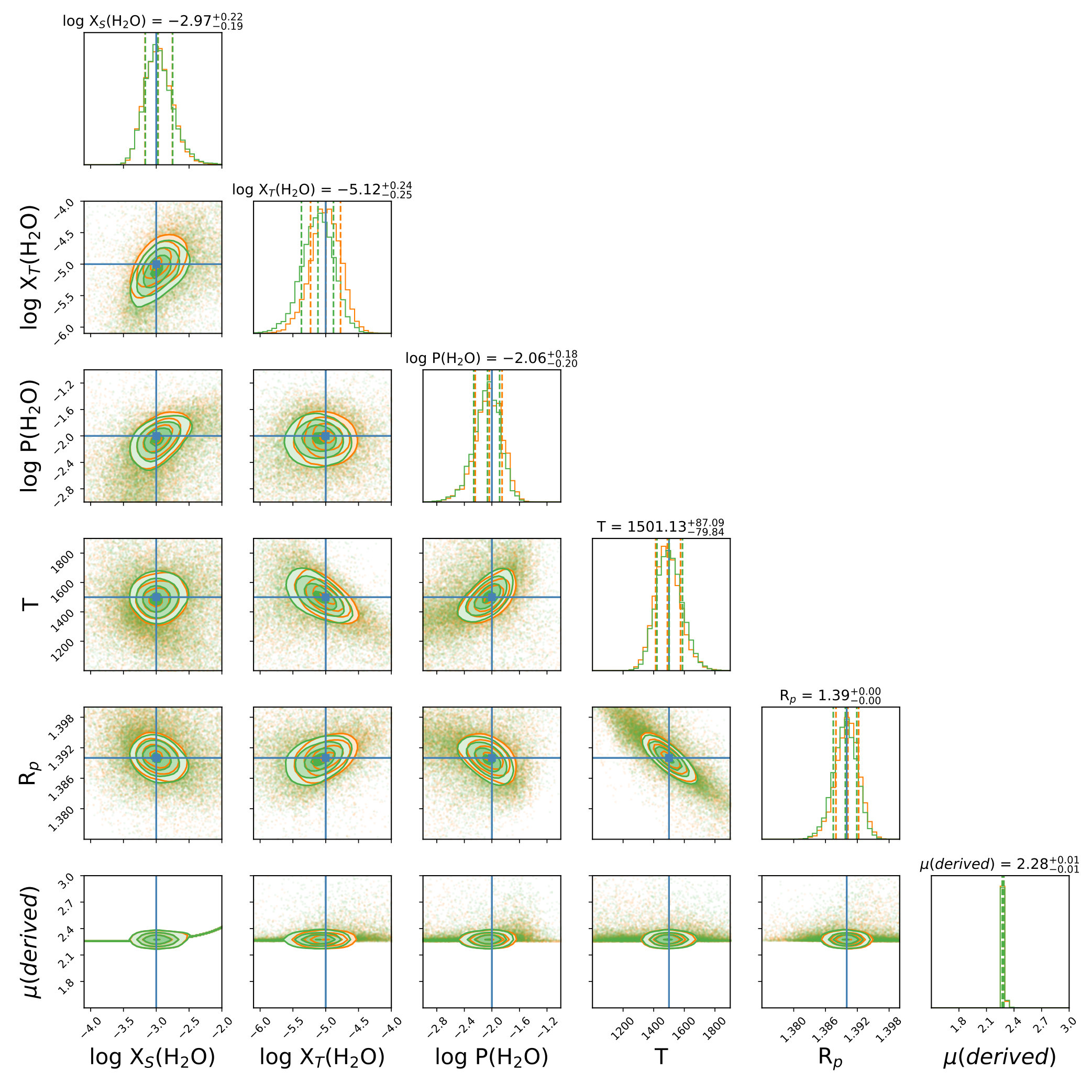 Figure 12
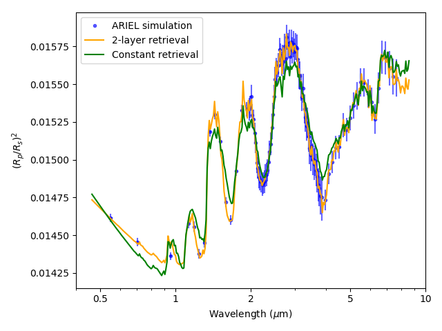 Figure 13
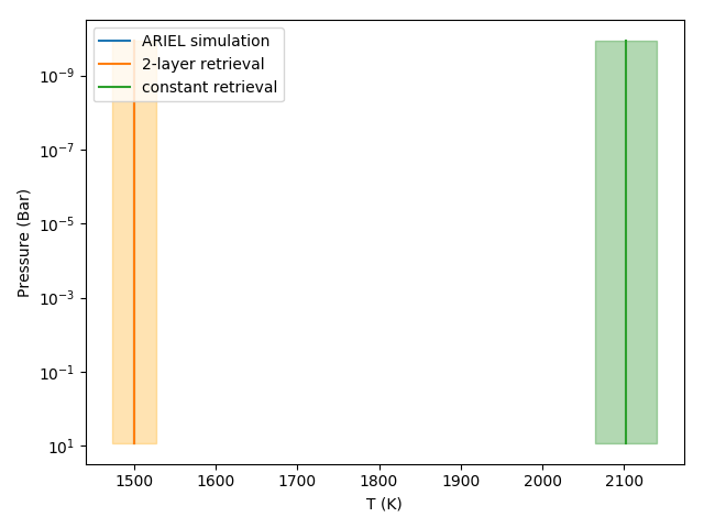 Figure 14
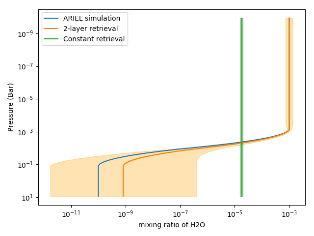 Figure 15
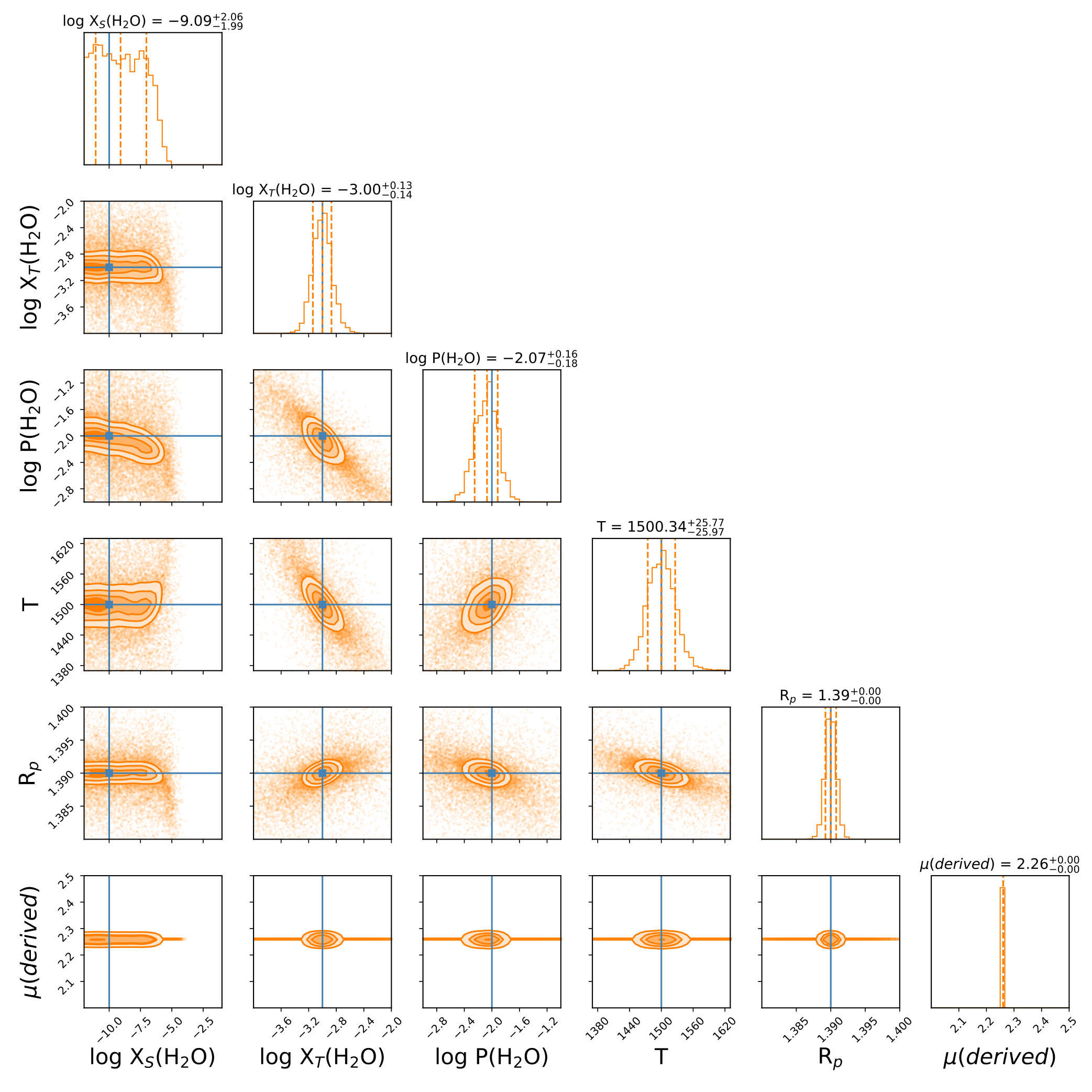 Figure 16
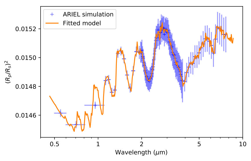 Figure 17
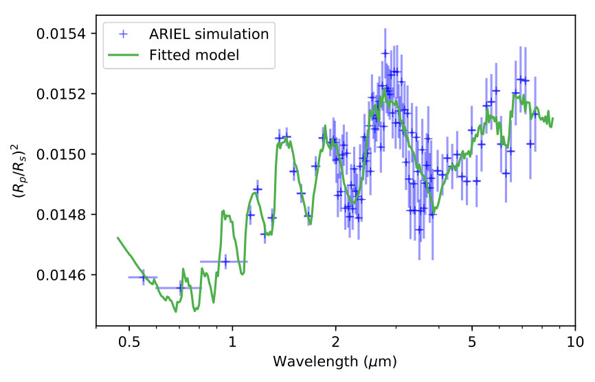 Figure 18
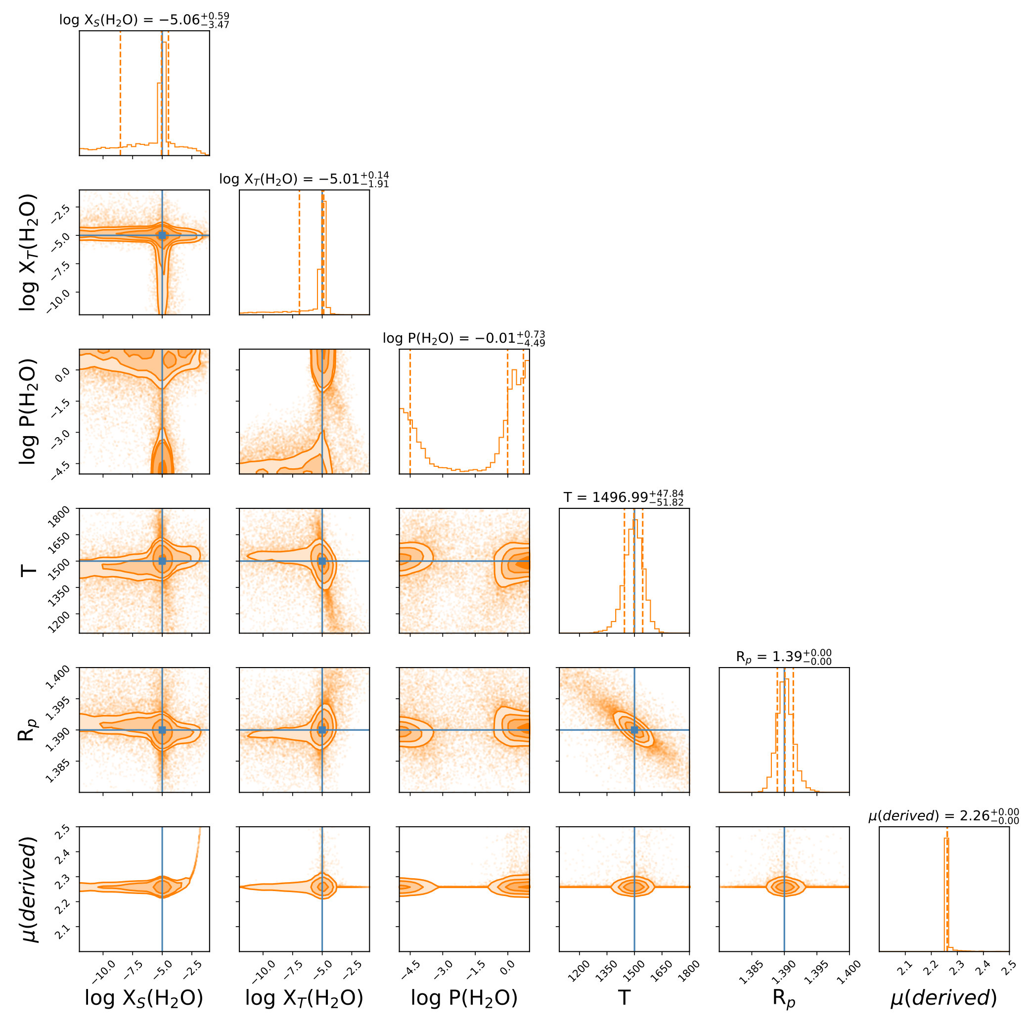 Figure 19
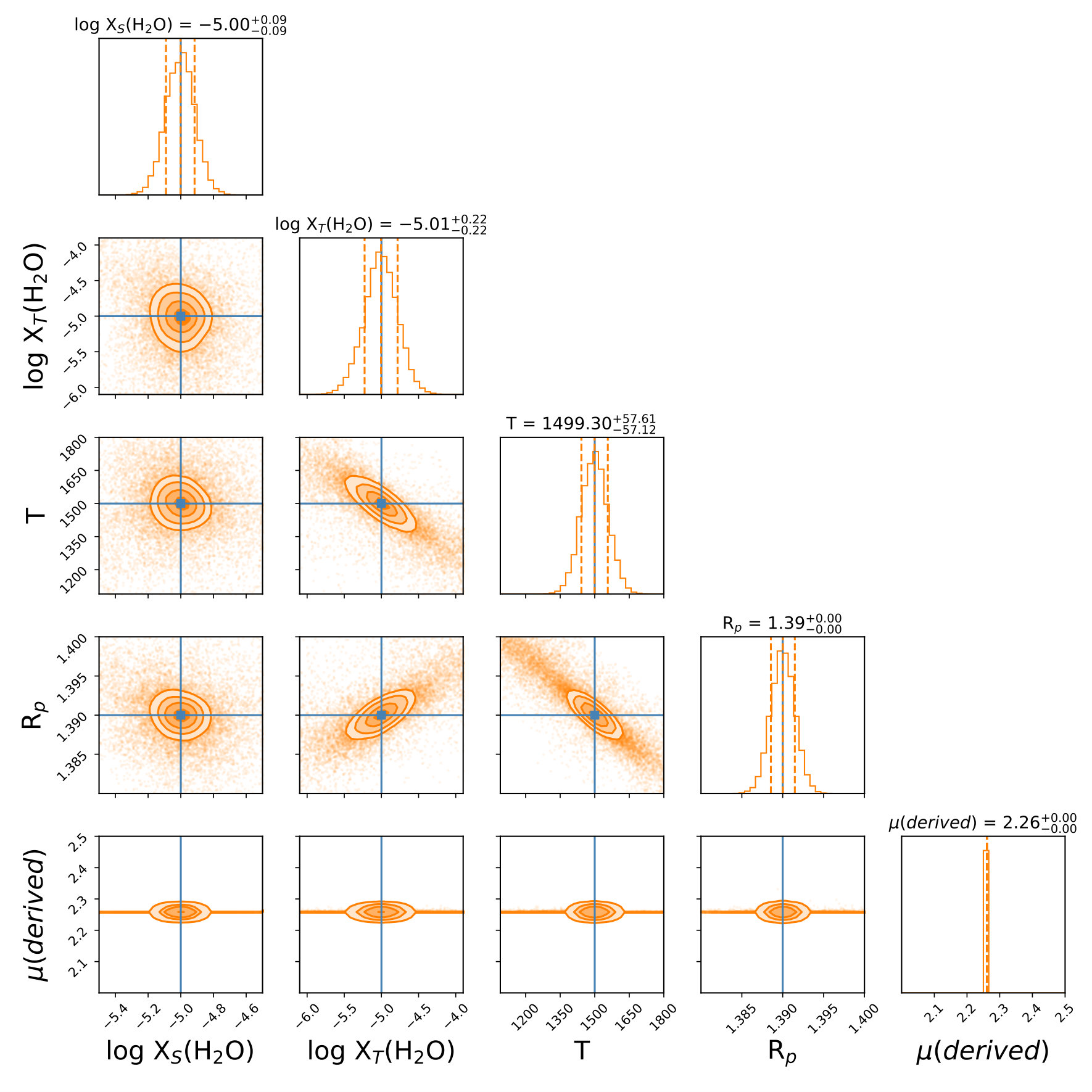 Figure 20
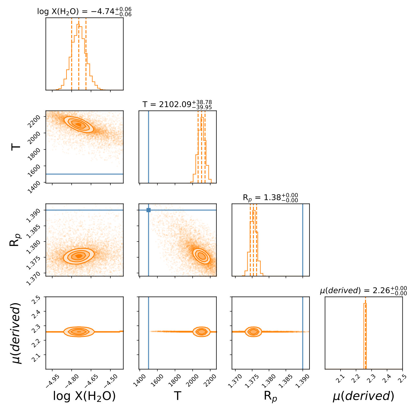 Figure 21
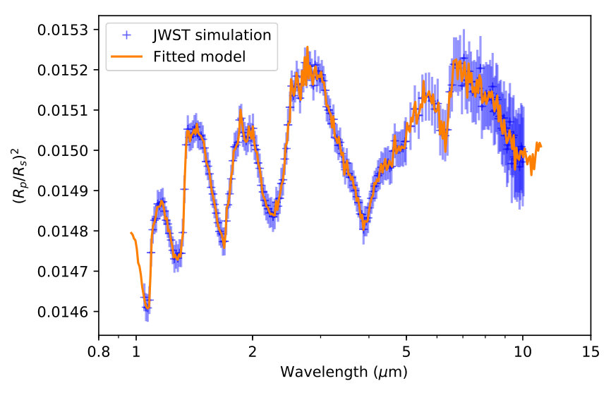 Figure 22
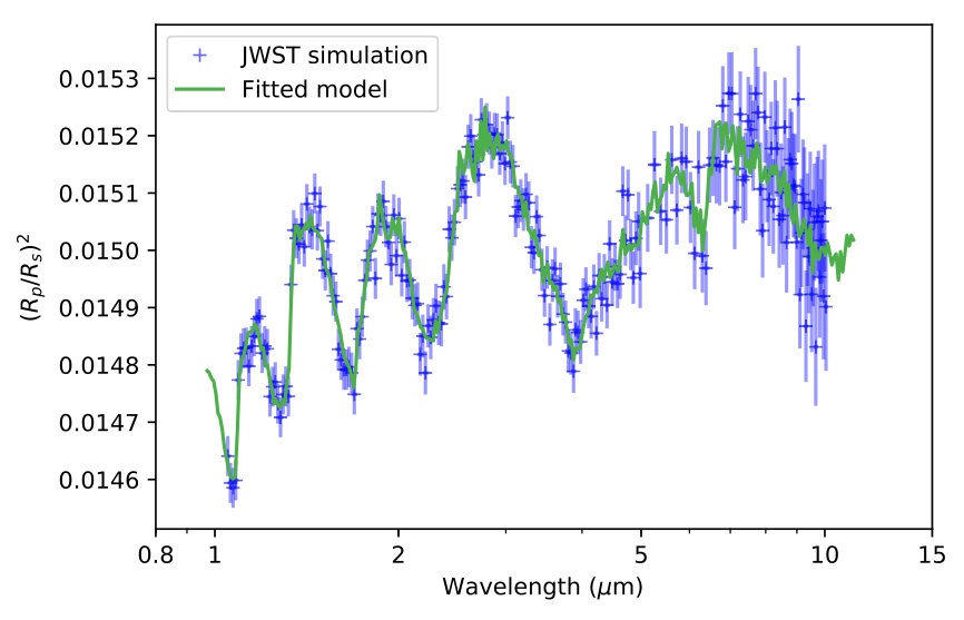 Figure 23
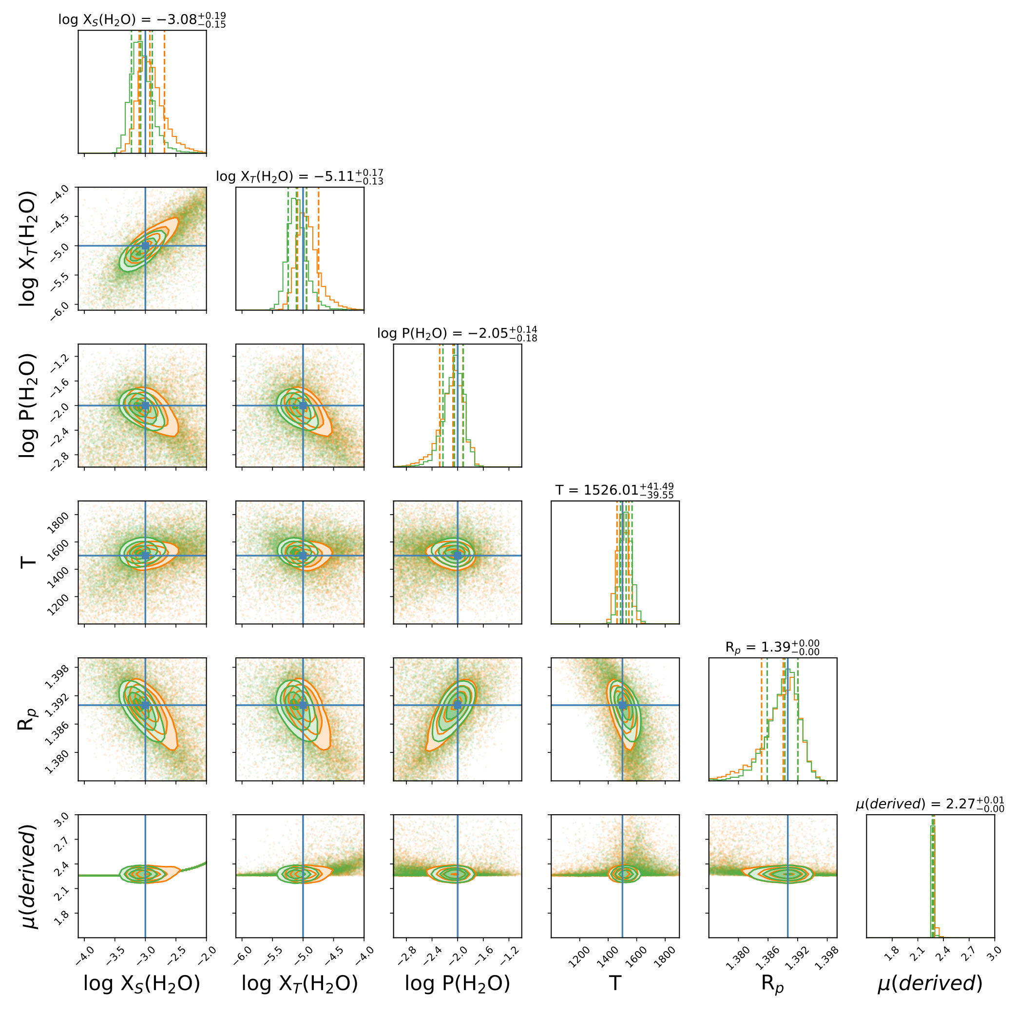 Figure 24
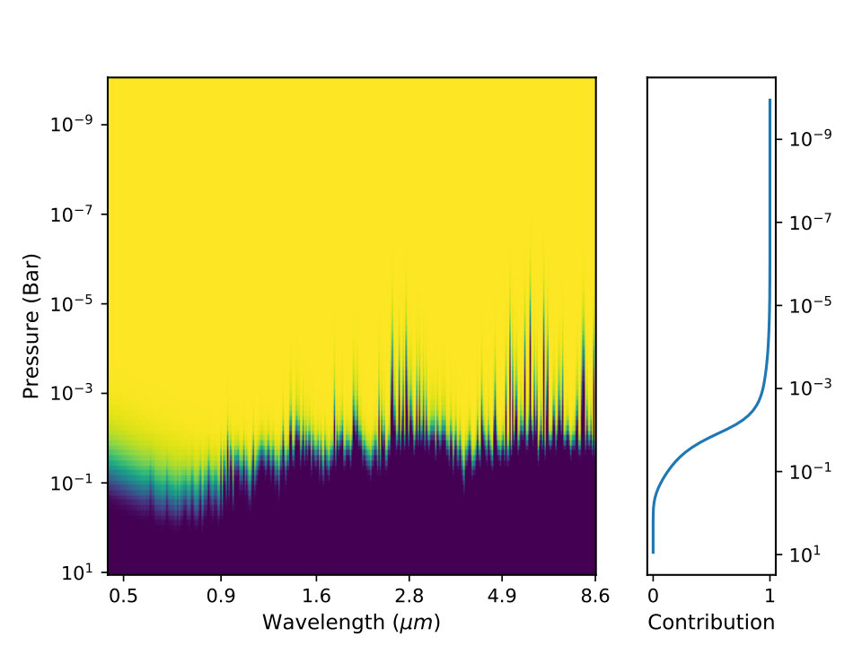 Figure 25
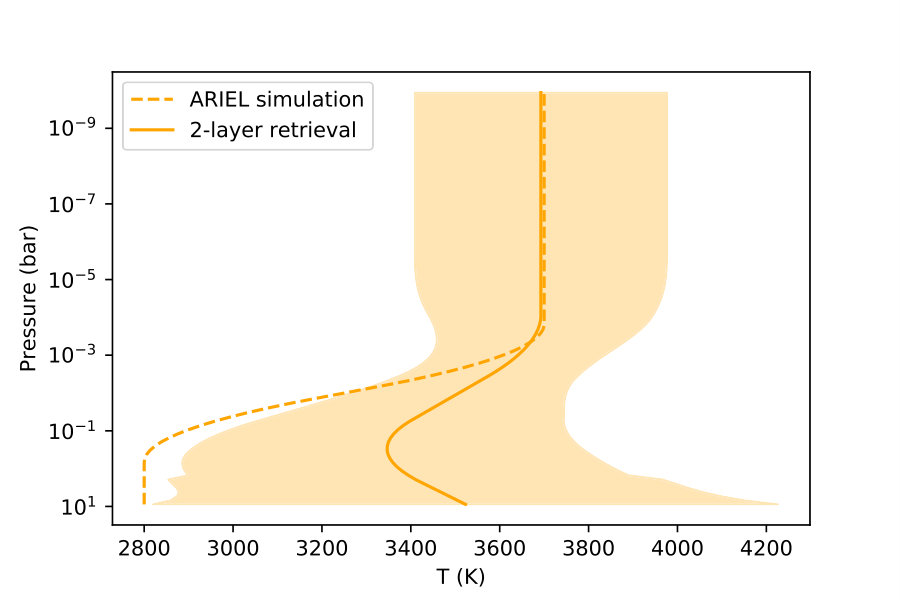 Figure 26
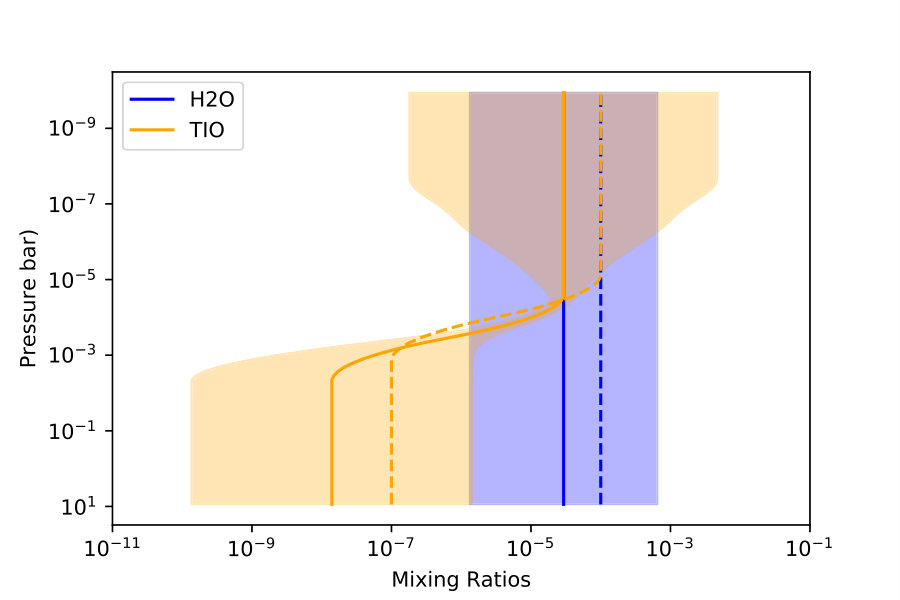 Figure 27
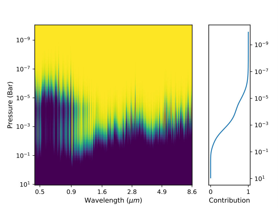 Figure 28
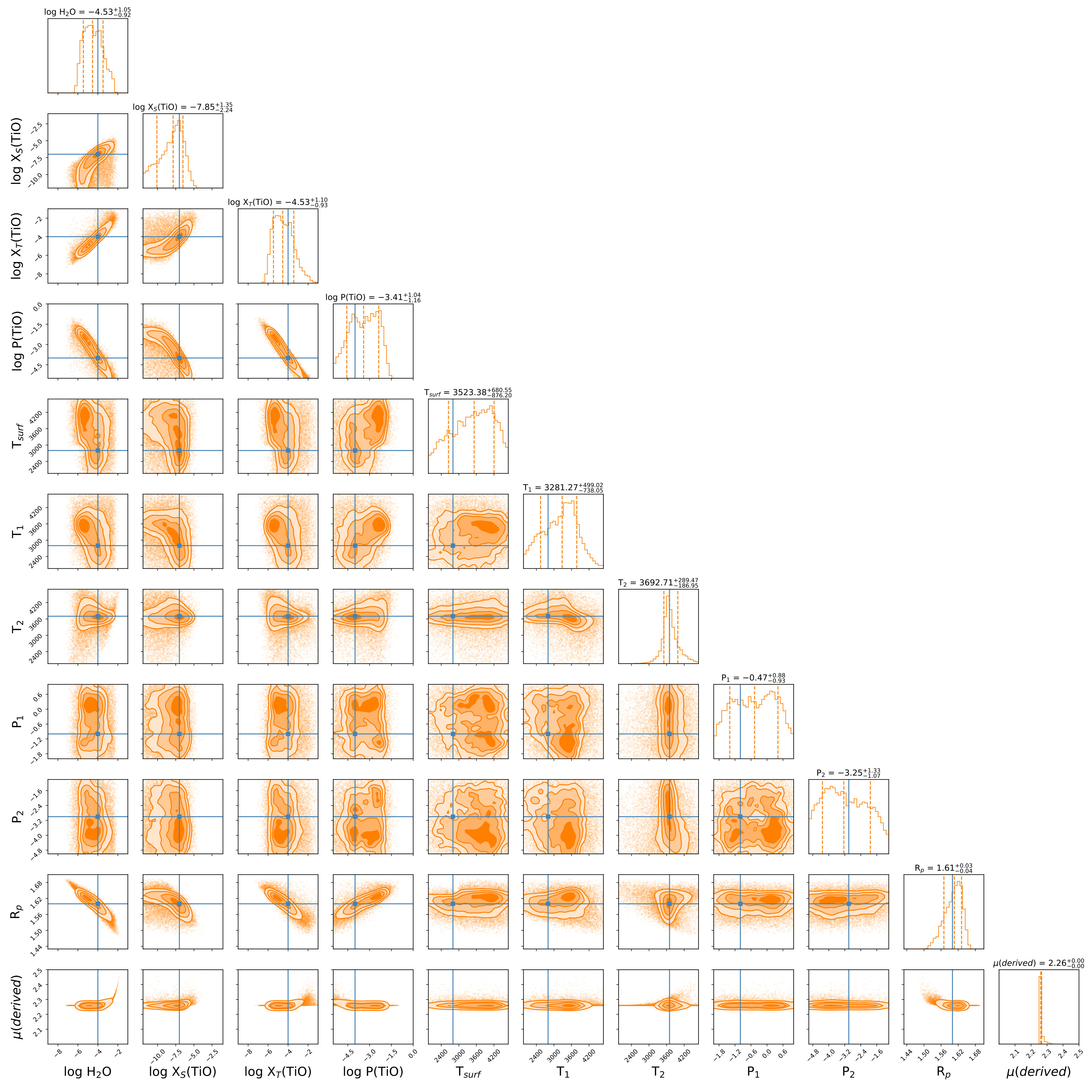 Figure 29
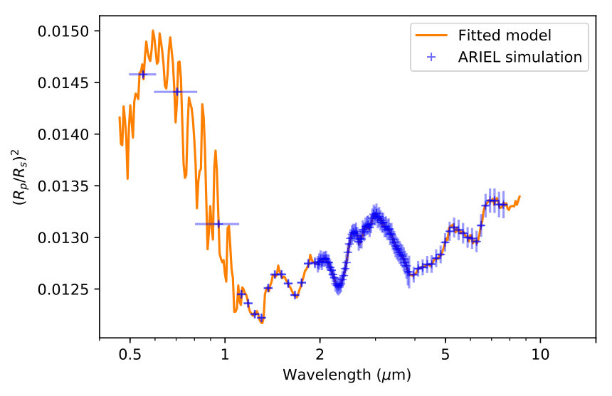 Figure 30
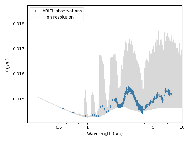 Figure 31
Peer Reviews
No public reviews on file for this paper yet. If you reviewed it on a platform where reviews are public (OpenReview, ICLR, NeurIPS, ICML), you can paste yours below so the community can read it here.
Videos
No videos yet. Explain this paper in a talk, walkthrough, or lecture? Add one.
Taxonomy
TopicsChemical and Environmental Engineering Research · SAS software applications and methods
Towards a more complex description of chemical profiles in exoplanet retrievals: A 2-layer parameterisation
Department of Physics and Astronomy
University College London
Gower Street,WC1E 6BT London, United Kingdom
Department of Physics and Astronomy
University College London
Gower Street,WC1E 6BT London, United Kingdom
Department of Physics and Astronomy
University College London
Gower Street,WC1E 6BT London, United Kingdom
Department of Physics and Astronomy
University College London
Gower Street,WC1E 6BT London, United Kingdom
(Accepted to ApJ, November 2019)
Abstract
State of the art spectral retrieval models of exoplanet atmospheres assume constant chemical profiles with altitude. This assumption is justified by the information content of current datasets which do not allow, in most cases, for the molecular abundances as a function of pressure to be constrained.
In the context of the next generation of telescopes, a more accurate description of chemical profiles may become crucial to interpret observations and gain new insights into atmospheric physics. We explore here the possibility of retrieving pressure-dependent chemical profiles from transit spectra, without injecting any priors from theoretical chemical models in our retrievals. The “2-layer” parameterisation presented here allows for the independent extraction of molecular abundances above and below a certain atmospheric pressure.
By simulating various cases, we demonstrate that this evolution from constant chemical abundances is justified by the information content of spectra provided by future space instruments. Comparisons with traditional retrieval models show that assumptions made on chemical profiles may significantly impact retrieved parameters, such as the atmospheric temperature, and justify the attention we give here to this issue.
We find that the 2-layer retrieval accurately captures discontinuities in the vertical chemical profiles, which could be caused by disequilibrium processes – such as photo-chemistry – or the presence of clouds/hazes. The 2-layer retrieval could also help to constrain the composition of clouds and hazes by exploring the correlation between the chemical changes in the gaseous phase and the pressure at which the condensed phase occurs.
The 2-layer retrieval presented here therefore represents an important step forward in our ability to constrain theoretical chemical models and cloud/haze composition from the analysis of future observations.
††software: TauREx (Waldmann et al., 2015a, b), ArielRad (Mugnai et al., 2020), Multinest (Feroz et al., 2009), Corner.py (Foreman-Mackey, 2016)
1 INTRODUCTION
In the past years an increasing number of exoplanetary atmospheres have been characterised with space and ground-based observatories. Ultraviolet, optical and infrared spectra, recorded through transit, eclipse, high-dispersion and direct imaging, have offered a glimpse of the atmospheric structure and composition of exotic worlds orbiting other stars. In most cases the data available are sparse and therefore their interpretation is rarely unique. To explore the degeneracy, reliability and correlations among the atmospheric parameters extracted from the data, the past decade has seen a surge in spectral retrieval models developed by many teams (e.g. Terrile et al., 2005; Irwin et al., 2008; Madhusudhan & Seager, 2009; Line et al., 2013; Waldmann et al., 2015b; Cubillos et al., 2016; Lavie et al., 2017; Goyal et al., 2018; Gandhi & Madhusudhan, 2018).
Most current spectral retrieval models assume constant or simplified atmospheric thermal profiles. Additionally, chemical profiles which are constant with altitude are assumed (e.g. MacDonald & Madhusudhan, 2017; Tsiaras et al., 2018; Pinhas et al., 2019). In these models, the mixing ratio of each individual molecule is fully determined by a single free parameter. So far, this approach has been successful due to the relatively poor quality of the input data from space and ground-based instruments. Given the low signal to noise, spectral resolution and the narrow wavelength coverage, current data cannot be used to constrain more complex models. However, the next generation of telescopes coming online in the next decade, will demand more complex retrievals to extract all the information content embedded in the data. In the context of NASA-JWST (Bean et al., 2018), ESA-ARIEL (Tinetti et al., 2018) and other facilities from ground and space (e.g. E-ELT (Brandl et al., 2018), Twinkle (Edwards et al., 2019b)), the higher resolution, signal-to-noise ratio (SNR) and broader wavelength range will allow for less abundant trace gases and refined thermal profiles to be captured. For instance, Rocchetto et al. (2016) have demonstrated that the assumption of constant atmospheric thermal profiles will be inadequate to interpret correctly future better-quality transit spectra recorded from space. Additionally these new instruments may be sensitive enough to constrain non-constant chemical profiles.
The need for an increased chemical complexity is sometimes addressed in the literature through additional constraints in the retrievals from dynamical and chemical models (“hybrid” models). This method is already widely explored in retrievals aiming at constraining the thermal profiles, e.g. the Guillot model (Guillot, 2010) and other 2-stream approximations (Heng et al., 2014; Malik et al., 2017). This strategy allows for more complex thermal profiles to be considered, while limiting the number of free parameters. Similarly, equilibrium and disequilibrium chemical models may be used to constrain chemical profiles. Agúndez et al. (2014) showed, with their 2D chemical model of HD 209458 b and HD 189733 b, that accurate parameterisations of exoplanetary atmospheres could be extremely complex. Interesting alternatives combine both physical/chemical models and free parameters such as the model adopted by Madhusudhan & Seager (2009), where the chemical profiles are computed in equilibrium and multiplied by a factor to account for potential departures from the equilibrium.
The hybrid retrieval models have, however, two major disadvantages. First, the forward model requires significant computing time to ensure convergence of the chemical/dynamical modules, which becomes even longer if used for retrievals. More fundamentally, they imply assumptions on the state of the planet and its physical/chemical behaviour. As the physics of such systems can be extremely complex and far from any environment we know in the Solar System, the selection of a particular model may lead to results biased by preconception. For instance, Venot et al. (2012) proposed a disequilibrium model adapted for hot-Jupiters and found significant differences when comparing with other models such as the equilibrium ones. This result highlights the issue of assuming a particular physics as a prior in inverse models, when our knowledge of exoplanetary atmospheres is still in an early phase. At least until our knowledge of these exotic worlds has progressed substantially, the results obtained by spectral retrievals should be kept independent from ab initio dynamical and chemical models, and used instead to constrain/validate some aspects of said models.
The approach taken here is to increase the number of free variables for each molecular species considered. Applying this approach to currently available data is not justifiable as it would simply increase the degeneracy of the retrieved solutions. By contrast, attempts to use models of inadequate complexity to analyse spectra observed by next generation facilities are likely to provide incomplete pictures and misleading results. This paper explores the importance of moving towards a more complete description of chemical profiles through the analysis of simulated transit data from JWST, ARIEL and other future telescopes. In that context, we consider the example of a 2-layer parametrisation with 3 degrees of freedom.
Section 2 presents the 2-layer approach and describes the methodology adopted. A validation of the method using simple cases is then reported in Section 3, followed by specific examples of exoplanetary atmospheres in section 4. Section 5 discusses the model’s strengths and limitations.
2 METHODOLOGY
2.1 Overview and key assumptions
This work focuses on retrievals of transit spectra, so that, for simplicity, the thermal profile can be assumed isothermal in some benchmark cases – note that this assumption is abandoned in Section 4 to ensure our simulations are as realistic as possible. In eclipse spectroscopy, the thermal gradients and the chemical profiles are always entangled, making it a more complex case which will be considered in a separate paper.
The 2-layer parametrisation has been adopted for its simplicity and because it does not rely on external physical assumptions which, as previously described, could bias the results of the retrieval. While our model is clearly not representative of all real atmospheres, it allows us to consider a departure from the constant mixing ratios case.
Both the forward radiative transfer models and the inverse models (spectral retrievals) are based on the open-source TauREx from Waldmann et al. (2015a) and Waldmann et al. (2015b), which has been modified for the purpose of this study. TauREx is a fully Bayesian radiative transfer and retrieval framework which encompasses molecular line-lists from the Exomol project (Tennyson et al., 2016), HITEMP (Rothman & Gordon, 2014) and HITRAN (Gordon et al., 2016). The complete list of opacity used in this paper can be found in Table 1. The public version of TauREx111https://github.com/ucl-exoplanets/TauREx_public is able to retrieve chemical composition of exoplanets by assuming constant abundances with altitude. It can also simulate atmospheres in equilibrium.
Here we added the new 2-layer module to the code. The chemical parametrisation we used can be described by three variables: the surface/bottom abundance , the top abundance and the pressure defining the separation of the two layers (Input Pressure Point for the forward model and Retrieved Pressure Point ). The chemical profile is linearly interpolated in log space – smoothing over 10% of the atmosphere – to avoid a sharp transition in the profile. An example of a 2-layer chemical profile for water vapour is given in Figure 1.
For all the tests reported in this paper, we follow the 3-step procedure detailed below.
2.2 Step 1: generating high-resolution input spectra
We start by using TauREx in forward mode and generate a high-resolution theoretical spectrum. In our models, we assumed a maximum pressure of bar, corresponding to the planet surface. The atmosphere is composed of the inactive gases H2 and He, for which we set the ratio He/H2 to 0.15 and add the considered active molecules (relative abundance defined by their mixing ratio). We consider collision induced absorption of the H2-H2 and H2-He pairs and opacities induced by Rayleigh scattering (Cox, 2015). Throughout the paper, the molecular mixing ratios and profiles in the forward model are varied to create high resolution spectra for a wide range of compositions and cases. The planetary parameters have been set to the well known exoplanet HD 209458 b in Section 3 and are listed in the Appendix. The adopted approach is compatible with any other set of planetary and atmospheric parameters and is applied in section 4 to two other simulated planets inspired by WASP-33 b and GJ 1214 b.
2.3 Step 2: convolution of the input spectra with the instrument response function
High-resolution theoretical spectra obtained in sec. 2.2 are convolved with the instrument response function to simulate realistic observations. We use ArielRad (Mugnai et al., 2020) to provide realistic noise models for spectra obtained by ARIEL and chose planets that are in the current target list Edwards et al. (2019a). In the case of JWST, we used the noise estimates for HD 209458 b presented in Rocchetto et al. (2016). An example of this process is shown in Figure 2 where both the high-resolution theoretical spectrum and the ARIEL-simulated case are presented.
2.4 Step 3: Retrievals
We run TauREx in retrieval mode and use the spectra obtained in step 2 as input to the retrieval. We used the nested sampling algorithm Multinest from Feroz et al. (2009) with 1500 live points and a log likelihood tolerance of 0.5. The retrieved parameters include our chemical setup (3 variables per chemical species), the isothermal temperature value and the planet radius. We therefore have a minimum of 5 free parameters that we attempt to retrieve. In the case where the mixing ratios were assumed constant with altitude (1-layer forward model), the Retrieved Pressure Point has been fixed, so that we have only 2 free variables per chemical species or a minimum of 4 free parameters. In our retrieval scheme, we use uniform priors for all the free parameters. In all our retrievals, chemical abundances are allowed to explore the bounds to . For the Retrieved Pressure Point, we allow the bounds from to bar for the Section 3. In Section 4, since we investigate less ad-hoc situations, we allow the pressure to explore bar to bar. For the isothermal temperature retrievals, the priors span 30 percent of the ground truth value. In section 4, since we investigate more realistic examples, we retrieve a 3-point temperature profile (Waldmann et al. (2015a)). The atmospheric parameters used to generate the theoretical spectrum in step 1 are the ground truth. By comparing the posteriors obtained by the retrieval to the ground truth, we can test the reliability and accuracy of the retrieval process. Furthermore, by using the predicted performances of JWST and ARIEL, we can quantify the expected information content of future data, with a view to assessing the ability to probe the chemical complexity of exoplanet atmospheres. For each retrieval, we state the Nested Sampling Log-Evidence. Bayes factor B (Jeffreys, 1998), which is the ratio of the evidences of two competing models ( and ), allows to compare models against each other. In practice, the table in Kass & Raftery (1995) gives an interpretation of :
By applying the 3-step methodology, a number of cases are simulated. Firstly, we verify that the 2-layer retrieval is able to recover the more basic 1-layer input (i.e. a constant chemical profile). We then investigate the “retrievability” of the 2-layer input spectrum by a 2-layer retrieval in the case of JWST and ARIEL observations. Finally, we explore the advantage of using a 2-layer approach by comparing how a 2-layer input spectrum is recovered by both 1- and 2-layer retrievals.
2.5 Testing the 2-layer approach: Retrieval of a 1-layer input spectrum using the 2-layer parametrisation
As a sanity check, we test that the more complex 2-layer model can indeed recognise the simple case of constant chemistry. A 1-layer simulated spectrum is generated and we attempt to recover the solution using the 2-layer model. Here, the retrieval of the pressure point () is disabled as this parameter introduces intrinsic degeneracy in the specific case of constant chemistry. Here, the goal being to illustrate that our 2-layer model returns the expected solution when tested on the 1-layer forward model, the behaviour of the retrieval when the Retrieved Pressure Point is activated is discussed in section 4. As any value for this point would work, we arbitrarily choose to set it at bar.
2.6 Retrieval of a 2-layer input spectrum as observed by JWST and ARIEL
We study an exoplanet exhibiting noticeable chemical modulations with altitude. This case can be simulated by using a 2-layer profile as input. We present the particular case of an input H2O profile with 2 layers separating at H2O bar. The input H2O surface layer is set with a mixing ratio of H2O and the top layer contains H2O. The input spectrum is simulated at high-resolution and observations are reproduced by convolving the theoretical spectrum to the instrument response function of JWST and ARIEL.
2.7 Comparison of the 1-layer and 2-layer retrievals.
By comparing the results obtained with the 1-layer and 2-layer retrievals, we aim to illustrate issues that may occur when performing a retrieval with a model of inappropriate complexity. Therefore, we simulate planetary atmospheres with 2-layer chemical profiles and analyse the results if the retrieval is performed with a 1-layer chemical approach. For this test, we use ARIEL simulations to illustrate our results. In particular, two main issues could occur and need to be tested:
The observed spectrum cannot be explained using the 1-layer retrieval, as the best solution retrieved does not fit the data. 2. 2.
The 1-layer retrieval manages to achieve a “good” fit but the retrieved parameters are wrong compared to the ground-truth. This issue is more subtle as there is little evidence and no direct way to spot the error.
These two points can be tested by considering the following examples. For the former, we assume an atmosphere with a single CH4 profile with a surface layer of CH up to CH bar and CH above that pressure, corresponding to a depleted layer. For the latter, we simulate a single H2O profile where the planet contains H2O up to bar and the mixing ratio is H2O for lower pressures.
3 RESULTS
3.1 Testing the 2-layer approach: Retrieval of a 1-layer input spectrum using the 2-layer parametrisation
The retrieved posterior distributions for an input spectrum generated with 1-layer parametrisation with a single species, H2O, is presented in Figure 3. In orange, we show the retrieved posterior distribution of the parameters, while the true value (when available) is marked in blue. The mixing ratio of H2O used for this example was . The 2-layer model successfully retrieved the same abundance for both layers. This result matches the single input parameter and confirms that the 2-layer parametrisation can recover the 1-layer input. This example showcases a situation where the complexity of the retrieval model is higher than the input.
3.2 Retrieval of a 2-layer input spectrum as observed by JWST and ARIEL
The input H2O surface layer was set as H2O and the top layer contained H2O. These abundances result in strong features in the spectrum but additional retrievals show that similar conclusions can be obtained for mixing ratios down to and for other molecules. The limits of the model are discussed in section 5. The planet parameters are retrieved for JWST and ARIEL using the 2-layer model. The best fitted spectra are presented in Figure 4 for the two telescopes. We also run the same cases with the noised up spectra, where we applied a dispersion corresponding to the uncertainties (see Figure 5). We show the posterior distributions of both cases for the JWST and ARIEL simulations in Figure 6.
The model is able to recognise the two layers in ARIEL and JWST simulations for the scattered and non-scattered cases.
Typically, to simulate an observation instance, the flux per wavelength observed, , is drawn from a Gaussian distribution (in the limit of being large) defined by its 1 error-bar and the “noise-free” mean flux of the forward model, . Here, we decided not to sample from this distribution and to adopt the ”noise-free” mean for the following reason. In this publication we are interested in the intrinsic biases resulting from using over-simplified to more complex (1-layer vs 2-layer) chemical profiles. To study these biases, one can either generate thousands of noise-instances, and average their retrieval results to obtain the underlying mean of the distribution, or avoid adding noise to in the first place. Given that in this case, all noise is Normally distributed and following the central-limit theorem (in the limit of large ) both approaches are equivalent. Feng et al. (2018) showed this to be the case and adopted the same rationale in their study. For the rest of the paper we therefore do not scatter our simulated spectra.
In the ARIEL case, we accurately retrieved both the surface layer (H2O)) and the top layer (H2O). The Retrieved Pressure Point also matched the input parameters (H2O bar). The same conclusions are reached for JWST. Additionally, in both simulations, the 2-layer retrievals recovered the correct temperature of 1500K and radius (1.39 ) corresponding to the input.
3.3 Comparison between the 1-layer and 2-layer retrievals.
We show here the results of the test where the input spectrum was generated assuming CH4 only with CH up to CH bar and CH. CH does not produce any observable feature, so for this layer we expect to retrieve only an upper limit in the posteriors. In this example, the 1-layer retrieval has difficulties in fitting the observed spectrum, as shown in Figure 7. In this case, the 1-layer retrieval lacks flexibility, which leads to a poor fit of the spectrum. This is also backed up by the lower Nested Sampling Global Evidence for the 1-layer scenario: 737 for the 1-layer and 885 for the 2-layer (). This example illustrates the need for a 2-layer retrieval.
Concerning the test where the input spectrum was generated with H2O only and assuming H2O and H2O above bar, both the 1-layer and 2-layer retrievals converged to a solution and gave a satisfactory fits of the input spectrum (See Figure 9). The posterior distributions are presented in Appendix, Figure 14. Unsurprisingly, the 2-layer retrieval managed to recover the correct input parameters. However, while fitting the spectrum, significant differences appear for the 1-layer model in the retrieved parameters. The 1-layer retrieval tries to compensate the lack of flexibility in the chemical profile by increasing the temperature to 2100K instead of the 1500K ground truth temperature. The input chemical and thermal profiles for both retrievals are shown in Figure 8.
The retrieved temperature by the 1-layer retrieval is significantly off compared to the input, while the retrieved H2O mixing ratio approximates the atmospheric average. This example illustrates well the importance of exploring and understanding more complex chemical models in retrievals. Here the retrieved spectrum using the 1-layer approximation (Figure 9) gives an acceptable fit while leading to a wrong solution, which is a serious issue. Small differences compared to the observations are noticeable which, in this case, would still permit the selection of the 2-layer solution, provided that both retrievals are performed. More importantly, the correct solution can be determined by comparing the Nested Sampling Global Log-Evidence of the retrieval. The 2-layer retrieval obtained a value of while the 1-layer only had , indicating a clear preference for the 2-layer scenario (difference of ).
4 More realistic examples
The previous sections demonstrated the theoretical possibility and, in some cases, the necessity of retrieving 2-layer chemical profiles in a number of select, simplified examples. Here we test the 2-layer approach by applying it to two cases inspired by GJ 1214 b and WASP-33 b. Spectra and parameters used in this section should not be considered as the “true” values of these real planets: they are realistic scenarios inspired from examples of the literature, which are here used to explore advantages and limitations of the 2-layer approach.
For instance, recent observations of the sub-Neptune GJ 1214 b in the near-IR unveiled a featureless spectrum, which could be caused by high-altitude hazes. Also, recent observations of the ultra hot-Jupiter WASP-33 b point towards a thermal inversion and a significant amount of TiO, which could cause this inversion by acting as a strong absorber in the visible. We simulate the WASP-33 b case with a 2-layer input model, while in the GJ 1214 b case we highlight the pertinence of our model by using the profiles from a disequilibrium chemistry model as input. We detail below all the assumptions we considered for our tests.
4.1 An ultra Hot-Jupiter inspired by WASP-33 b
Current analyses of ground and space-based observations of WASP-33 b suggest extreme temperatures reaching 3800 K and a possible thermal inversion in the atmosphere (Haynes et al., 2015; Nugroho et al., 2017). TiO or VO, which are strong absorbers at short wavelengths, could very efficiently capture high-energy stellar photons at the top of the atmosphere and cause the inversion (Fortney et al., 2008; Spiegel et al., 2009). In parallel, other observations have suggested the presence of TiO in Wasp-121 b (Evans et al., 2017) and Wasp-76 b (Tsiaras et al., 2018).
Here we investigate this process by attempting to detect a TiO layer in the upper atmosphere of a simulated planet resembling WASP-33 b. Our input model includes only two molecules: H2O and TiO. The simulation consists of a constant mixing ratio of for H2O and an inverted temperature-pressure (TP) profile from 2800K to 3700K, which is inspired by Haynes et al. (2015). For the temperature-pressure profile we used a 3-point model (Waldmann et al., 2015a). This model interpolates a smooth TP profile using 5 free parameters, i.e. surface temperature and two temperature-pressure points. The temperature variations allow us to explore the possibility of retrieving both thermal and chemical parametric profiles at the same time. Rocchetto et al. (2016) have shown that non-isothermal profiles could introduce a bias in JWST observations. This is also expected to be true for ARIEL and we can investigate it as a side result of this work. For the retrieval, we explore uniform priors on the pressure bounds - bar for the point 1 and - bar for the point 2. The temperature bounds are the same for all 3 retrieved points and cover the a range 30 percent lower/higher than the input min/max temperatures (1960K - 4690K). For a real observation, these priors could be informed by the knowledge of the equilibrium temperature and the physics of the atmosphere. To simulate a stratospheric TiO layer, we assumed abundances of TiO for the top layer (down to bar) and TiO at the surface. The spectrum, as well as the temperature and chemical profiles, are presented in Figure 10 while the full posterior distribution is available in the Appendix, Figure 15.
These results demonstrate the possibility of accurately retrieving the vertical distribution of the TiO layer. In particular, the TiO profile is well constrained between bar and bar as a result of the strong features between 0.4 and 1 . The shape of the thermal profile is also correctly retrieved, although with a larger uncertainty at higher pressures as shown by the posterior distribution. The retrievability of the thermal and chemical profiles at the same time indicates that retrievals of future transit spectra should take these two effects into account. The flexibility of the 2-layer approach allows for the confirmation (or rejection) of potential correlations between molecules/condensates and thermal inversions. This is an important application of the 2-layer approach.
4.2 A warm sub-Neptune inspired by GJ 1214 b
As previously mentioned, GJ 1214 b is a sub-Neptune with a relatively flat spectrum in the visible and near-infrared. Multiple explanations for the lack of features have been proposed (Miller-Ricci Kempton et al., 2012; Morley et al., 2013; Kreidberg et al., 2014):
- •
The planet could have an atmosphere heavier than hydrogen, such as a water dominated atmosphere.
- •
The atmosphere could be hydrogen dominated with opaque, high altitude clouds (e.g. KCl or ZnS).
- •
The planet could have hydrocarbon hazes in the upper atmosphere.
Here we investigate the retrievability of the third scenario as an example of 2-layer chemistry. The photo-chemical hazes could be similar to those found in the atmosphere of Saturn’s moon Titan. CH4 in the upper atmosphere is photolysed by radiation, creating hydrocarbon hazes that are opaque in the near infrared. This scenario implies a significant CH4 abundance at the surface of the atmosphere and a sharp decline in the upper atmosphere. For our input forward model, we used the chemical profiles of the four molecules H2O, CH4, CO2 and CO published by Miller-Ricci Kempton et al. (2012) in the case of solar abundance and . The profiles are retrieved using two scenarios: A hybrid one with 2-layer chemistry for H2O and CH4 and the 1-layer for CO2 and CO; and a fully 1-layer chemistry with all 4 molecules retrieved using constant profiles. For the hybrid case, the abundances of CO2 and CO were indeed too low to retrieve the 2-layer profile. The other input parameters for the planet are described in the Appendix. We add hydrocarbon hazes layer adopting the model described in Lee et al. (2013). The clouds are treated as additional opacity for each layer of size :
[TABLE]
Where is the size of the cloud particles and is the cloud number density. Here the extinction efficiency has been defined as:
[TABLE]
and the cloud size parameter is:
[TABLE]
In the forward model, the particle size was assumed to be 0.01 microns while was set to . We also simplify our problem by assuming the hazes cover the entire atmospheric pressure range. The parameter describes the type of clouds and is, in this example, fixed to the value of 80 as it can be informed from theoretical models. The bounds of the cloud parameters are chosen to cover a wide range of possibilities: varies between 0.003 - 1 and varies between - . As with WASP-33 b, we chose a 3-point thermal profile and apply the same bounds (490K - 1690K). For these two cases, the full posteriors are presented in Appendix Figure 16 and Figure 17. The fitted spectrum, the chemical profiles and the TP profile are presented in Figure 11.
We find that for the 2-layer hybrid scenario, all input chemical parameters except the abundance of CO can be recovered. Due to the high opacity, we retrieve weak constraints on the temperature parameters at high pressure, returning large posteriors for , and the associated pressures. The cloud parameters are retrieved within the expected values. We notice a strong correlation between the clouds particle size and their abundances.
In the full 1-layer scenario, the solution provides a good fit to the observation, while the retrieved abundances for H2O and CH4 seem to average the real profiles. However, it appears that the temperature profile exhibit large variations, especially for pressures lower than bar, where the true temperature profile is outside the retrieved 1-sigma temperature. The difficulty encountered by the 1-layer scenario in explaining the spectrum is also confirmed by the retrieved posteriors in Appendix Figure 17 where, in particular, the temperature and pressure of point 2 are offset from the true values and are degenerate with the other parameters. We also find that the radius is not as well retrieved as in the 2-layer hybrid case. In practice, the 1-layer solution would be unlikely to be accepted since the retrieved temperature points tend to push towards values outside reasonable priors.
This result confirms that the isothermal assumption could lead to biases in retrievals of JWST and ARIEL (Rocchetto et al., 2016). Additionally, the mixing ratio of around of H2O in the upper atmosphere is too low to be captured by observations given the large haze opacity assumed. For this planet, the detection limit of H2O at this altitude is around , correctly interpreted by the large error bars. Also for this example, by using a 2-layer retrieval, correlations in the chemical profiles and detection of cloud layers in transit spectra could inform us about the nature of hazes and clouds.
5 DISCUSSION
5.1 A physically motivated reason to consider non-constant vertical chemical profiles
We have shown in the previous sections that simulated atmospheres with a 2-layer chemical profile would induce spectral features that need to be properly accounted for in retrievals to avoid incorrect conclusions. However, one could ask whether such family of chemical profiles can be found in exoplanetary atmospheres. We have already demonstrated through the cases of WASP-33 b and GJ 1214 b that chemical profiles with vertical discontinuities could be important if clouds and hazes are present in the atmosphere.
Additionally, chemical simulations by Venot et al. (2012) suggest at least two typical behaviours for chemical profiles in exoplanetary atmospheres of the type HD 209458b. Some molecules of interest, such as H2O and CO, are predicted to have a constant mixing ratios as a function of pressure. Others, like NH3 or CH4, are expected to vary with altitude. In the deep atmosphere (generally pressures higher than bar / Pa) chemical reactions are close to their thermochemical equilibrium values. In the higher part of the atmosphere ( bar / Pa) photo-chemistry and disequilibrium processes may modify the overall mix by dissociation and creation of atomic species and new molecules. In addition, Moses et al. (2013) investigated the composition of Hot Neptunes like GJ 436 b with a wide range of metallicities and the resulting chemical profiles demonstrated complex behaviours. This highlights the need for adapted retrieval techniques. These disequilibrium processes are expected to be more prominent and important in colder atmospheres (Tinetti et al., 2018).
Future space instruments should be able to probe roughly between bar and bar, depending on the composition and temperature of the atmosphere, allowing to constrain chemical models with direct observations. This is showcased in Figure 12, where the plots illustrate the contribution functions and their wavelength dependencies for planets similar to HD 209458 b, WASP-33 b and GJ 1214 b.
5.2 Should we always use the 2-layer model?
The increase in complexity in chemical models must be done with care. In some cases, the introduction of additional degrees of freedom comes at the expense of model convergence, i.e: the flexibility of the retrieval should depend on the quality of the input data. This opens up the question of model selection. Indeed, should we prefer models with increased flexibility at the risk of increasing model degeneracies and over-fitting, or should we prefer simpler models but returning only “acceptable” fits?
In the 2-layer case, this issue can be illustrated by the retrieval of a constant input. In section 3.1, we disabled the Retrieved Pressure Point to ensure the convergence of the 2-layer retrieval. This choice was justified by the fact that the Input Pressure Point does not exist in constant chemical profiles, making any Retrieved Pressure Point suitable and therefore introducing an intrinsic degeneracy. In Figure 13 the constant chemical profile used as input is here retrieved with the Retrieved Pressure Point activated (log P(H2O)). The point is however not well constrained and the retrieved abundances become more difficult to interpret. The posteriors are compatible with a bi-modal solution peaked at pressures where observations are no longer sensitive.
This example highlights the circumstances under which the model used in the retrieval is too complex. The issue was solved previously in Figure 3 by fixing the Retrieved Pressure to an arbitrary value (reduction of the model complexity), illustrating that if/when the 2-layer model is too complex for the data, one needs to decrease the number of free parameters and revert back to a simpler chemical parameterisation. This can clearly be seen from the posterior distribution (namely the pressure point divergence).
6 CONCLUSIONS
In this paper we have assessed the possibility of constraining the abundance as a function of altitude of key chemical species present in exoplanet atmospheres. We have used simulated JWST and ARIEL transit spectra to test whether the data quality of the next generation of space-based instruments will allow for the retrieval of vertical chemical profiles. The 2-layer model assumed in our paper, while still being a coarse approximation of the real case, provides an increased level of complexity and flexibility in the interpretation of the data compared to the assumption of constant abundance for each chemical species. To test the validity and usefulness of the model, we included the 2-layer method in the spectral retrieval algorithm TauREx and performed the retrieval of JWST- and ARIEL-like transit spectra generated by assuming both ad hoc, simplified atmospheric examples and more realistic cases.
We found that the 2-layer retrieval is able to capture accurately discontinuities in the vertical chemical profiles, which could be caused by disequilibrium processes – such as vertical mixing or photo-chemistry – or the presence of clouds/hazes. Our approach should therefore help the removal of the hurdles in interpreting observational constraints that have hindered the confirmation of current chemical models published in the literature. Additionally, the 2-layer retrieval could help to constrain the composition of clouds and hazes by studying the correlation between the chemical changes in the gaseous phase and the pressure at which the condensed/solid phase occurs. This result is particularly important given that clouds/hazes have been detected in half of the currently available exoplanet spectra, but their composition is still elusive as it cannot be inferred directly through remote sensing measurements.
Future work will extend this analysis to eclipse spectra and explore the need for more complex vertical profiles.
Acknowledgements
This project has received funding from the European Research Council (ERC) under the European Union’s Horizon 2020 research and innovation programme (grant agreement No 758892, ExoAI), under the European Union’s Seventh Framework Programme (FP7/2007-2013)/ ERC grant agreement numbers 617119 (ExoLights) and the European Union’s Horizon 2020 COMPET programme (grant agreement No 776403, ExoplANETS A). Furthermore, we acknowledge funding by the Science and Technology Funding Council (STFC) grants: ST/K502406/1, ST/P000282/1, ST/P002153/1, ST/T001836/1 and ST/S002634/1.
Planet’s parameters used for the forward models
Parameters used in our forward models for the 3 types of planets: a hot-Jupiter type HD 209458 b (Stassun et al. (2017)), an Ultra hot-Jupiter type WASP-33 b (Stassun et al. (2017)) and a Sub Neptune Type GJ 1214 b (Harpsøe et al. (2013)):
[TABLE]
Posteriors of retrievals for a planet with an inverted H2O chemical profile using constant and 2-layer chemical models
Posteriors distribution for the retrieval of WASP-33 b
Posteriors distribution for the retrieval of GJ 1214 b with 2-layer profiles for H2O and CH4 and constant profiles for CO2 and CO
Posteriors distribution for the retrieval of GJ 1214 b in the case of constant chemical profiles
The reference list from the paper itself. Each links out to its DOI / PubMed record.
- 1Abel et al. (2011) Abel, M., Frommhold, L., Li, X., & Hunt, K. L. 2011, The Journal of Physical Chemistry A, 115, 6805
- 2Abel et al. (2012) —. 2012, The Journal of chemical physics, 136, 044319
- 3Agúndez et al. (2014) Agúndez, M., Parmentier, V., Venot, O., Hersant, F., & Selsis, F. 2014, A&A, 564, A 73
- 4Barton et al. (2017) Barton, E. J., Hill, C., Yurchenko, S. N., et al. 2017, Journal of Quantitative Spectroscopy and Radiative Transfer, 187, 453
- 5Bean et al. (2018) Bean, J. L., Stevenson, K. B., Batalha, N. M., et al. 2018, Publications of the Astronomical Society of the Pacific, 130, 114402
- 6Brandl et al. (2018) Brandl, B. R., Absil, O., Agócs, T., et al. 2018, in Society of Photo-Optical Instrumentation Engineers (SPIE) Conference Series, Vol. 10702, Ground-based and Airborne Instrumentation for Astronomy VII, 107021 U
- 7Cox (2015) Cox, A. N. 2015, Allen’s astrophysical quantities (Springer)
- 8Cubillos et al. (2016) Cubillos, P., Blecic, J., Harrington, J., et al. 2016, BART: Bayesian Atmospheric Radiative Transfer fitting code, Astrophysics Source Code Library, , , ascl:1608.004