TL;DR
This paper analyzes the statistical properties of the network Lasso (nLasso) for localized linear regression on networked data, providing conditions for accurate learning from limited labels and an implementation via primal-dual methods.
Contribution
It offers a theoretical analysis of nLasso's ability to learn localized linear models with few labels and presents a specialized implementation using primal-dual optimization.
Findings
Identifies sufficient conditions on network structure and labels for accurate nLasso learning.
Provides a scalable primal-dual algorithm for localized linear regression with nLasso.
Demonstrates the effectiveness of nLasso in networked data scenarios.
Abstract
The network Lasso (nLasso) has been proposed recently as an efficient learning algorithm for massive networked data sets (big data over networks). It extends the well-known least absolute shrinkage and selection operator (Lasso) from learning sparse (generalized) linear models to network models. Efficient implementations of the nLasso have been obtained using convex optimization methods lending to scalable message passing protocols. In this paper, we analyze the statistical properties of nLasso when applied to localized linear regression problems involving networked data. Our main result is a sufficient condition on the network structure and available label information such that nLasso accurately learns a localized linear regression model from a few labeled data points. We also provide an implementation of nLasso for localized linear regression by specializing a primaldual method for…
Click any figure to enlarge with its caption.
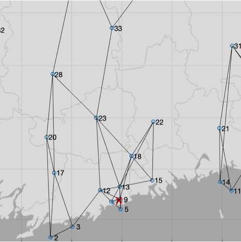 Figure 1
Peer Reviews
No public reviews on file for this paper yet. If you reviewed it on a platform where reviews are public (OpenReview, ICLR, NeurIPS, ICML), you can paste yours below so the community can read it here.
Code & Models
Videos
No videos yet. Explain this paper in a talk, walkthrough, or lecture? Add one.
Taxonomy
MethodsLinear Regression
Localized Linear Regression in Networked Data
Alexander Jung and Nguyen Tran Authors are with the Department of Computer Science, Aalto University, Finland; firstname.lastname(at)aalto.fi
Abstract
The network Lasso (nLasso) has been proposed recently as an efficient learning algorithm for massive networked data sets (big data over networks). It extends the well-known least absolute shrinkage and selection operator (Lasso) from learning sparse (generalized) linear models to network models. Efficient implementations of the nLasso have been obtained using convex optimization methods lending to scalable message passing protocols. In this paper, we analyze the statistical properties of nLasso when applied to localized linear regression problems involving networked data. Our main result is a sufficient condition on the network structure and available label information such that nLasso accurately learns a localized linear regression model from a few labeled data points. We also provide an implementation of nLasso for localized linear regression by specializing a primal-dual method for solving the convex (non-smooth) nLasso problem.
I Introduction
The data arising in many important application domains can be modeled efficiently using some network structure. Examples of such networked data are found in signal processing where signal samples can be arranged as a chain, in image processing with pixels arranged on a grid, in wireless sensor networks where measurements conform to sensor proximity [1, 2, 3, 4]. Organizing data using networks is also used in knowledge bases (graphs) whose items are linked by relations [5, 6].
In what follows, we will represent networked data using an undirected “empirical graph”. The nodes of the empirical graph represent individual data points (e.g., one image out of an entire collection) which are connected by edges according to some notion of similarity. This similarity might be induced by domain knowledge (e.g., friendship relations in social networks) or via probabilistic models ( [7, 8].
Beside their network structure, data points are typically characterized by features and labels. The features of data points are quantities that can be measured or computed efficiently (in an automated fashion). In contrast, the labels of data points are costly to acquire, involving human expert labor.
We consider regression problems within which data points are characterized by features and a numeric label (or target). The goal is to learn an accurate predictor which maps the features of a data point to a predicted label. The learning of the predictor is based on the availability of a few data points with known labels. Facing partially labeled data is common since the acquisition of reliable label information is often costly (involving human expert labor).
Accurate learning is particularly challenging in the high-dimensional regime [9, 10]. Here, a key obstacle is the lack of a sufficient amount of samples which can be considered i.i.d. Using a network structure allows then to borrow statistical strength from different “groups” of samples which are not exactly i.i.d., but still statistically similar to some extent.
The learning of an accurate predictor from a small number of labeled data points is enabled by exploiting the tendency of well-connected data points to have similar statistical properties. Such a clustering assumption, which underlies most (semi-) supervised machine learning methods [11, 12], requires any reasonable predictor to be nearly constant over well-connected subsets (clusters) of data points. The clustering assumption motivates the network Lasso (nLasso) as a form of empirical risk minimization [13].
Contribution. While several implementations of nLasso have been proposed and analyzed (see [13, 14]), little is known about the accuracy of nLasso in regression problems. The main contribution of this paper is a sufficient condition on the network topology and available label information such that the nLasso accurately learns a predictor from a small number of labeled data points. To this end, we apply (an extension of) the network compatibility condition (NCC) introduced in [15].
We demonstrate theoretically and empirically, that the NCC guarantees that nLasso learns an accurate predictor which conforms with the clustering hypothesis. Our theoretical findings help to design sampling schemes which identify those data points whose labels would provide the most information about the labels of the other data points [16, 4].
Notation. The identity matrix of size is denoted . The positive part of some real number is . The Euclidean norm of a vector is . For a positive definite matrix , we define the induced norm . We will need the vector-valued clipping function for and otherwise. The soft-thresholding operator is .
II Problem Formulation
We consider networked data modelled by an undirected “empirical” graph whose nodes represent individual data points. The undirected edges encode some domain-specific notion of similarity between data points. The similarity between nodes connected by the edge is quantified by a positive edge weight . We collect the weights (with if nodes are not connected by an edge), into the weight matrix .
In addition to the graph structure , datasets typically convey additional information about the data points. Let us assume that each individual data point is characterized by a feature vectors and a numeric label . The features can be determined easily for any data point. In contrast, acquisition of labels is difficult (requiring human expert labor). Our approach allows to have access only to the labels of a small training set .
We relate features and labels using the linear model
[TABLE]
with some (unknown) weight vector for each node . The noise component in (1) summarizes any labeling our modeling errors.
Thus, we assign each data point with an individual linear model (1). For high-dimensional data (feature vector length ) this would result in overfitting unless we leverage the information contained in the network structure relating different data points. As we demonstrate theoretically and empirically, enforcing the (estimates of the) weight vectors to be similar for well-connected data points allows to accurately learn the linear models (1) for the entire dataset.
We will apply nLasso to the available labels for the training set to obtain an estimate for the weight vector at each node . The estimates define a predictor which maps the node to the predicted label
[TABLE]
The predictions will be accurate, i.e., the prediction error will be small, if the estimation error is small. Our main result (see Theorem 2) provides a sufficient condition on the structure of the empirical graph and the training set such that the estimation error is small.
We interpret the weight vectors as the values of a graph signal which assigns node the vector . The set of all vector-valued graph signals is denoted
[TABLE]
Each graph signal represents a predictor which maps a node with features to the predicted label (2).
Given partially labeled networked data, we aim at leaning a predictor whose predictions (2) agree with the labels of labeled data points in the training set . In particular, we aim at learning a predictor having a small training error
[TABLE]
We use the absolute value loss since it somewhat simplifies our analysis. However, we expect no big challenges in extending our analysis to nLasso using different loss functions, such as the squared error loss. The absolute value loss is actually preferred for learning linear regression models (1) when the noise is expected to contain only a few large values, known as “salt and pepper” noise in image processing [17].
III Network Lasso
The criterion (4) by itself is not enough for guiding the learning of a predictor since (4) completely ignores the weights at unlabeled nodes . Therefore, we need to impose some additional structure on the predictor . To this end, we require the predictor to conform with the cluster structure of the empirical graph [18, 19].
The extend by which a predictor conforms with can be measured by the total variation (TV)
[TABLE]
If the weights are approximately constant over well-connected subsets of nodes, the predictor has small TV . The restriction of (5) to a subset of edges is denoted .
We are led naturally to learning a predictor via the regularized empirical risk minimization (ERM)
[TABLE]
which is a special case of nLasso [13]. The parameter in (6) allows to trade small TV against small error (4). The choice of can be guided by cross validation [20]. Alternatively the choice of can be guided by our analysis of the nLasso estimation error (see discussion after Theorem 2).
Note that nLasso (6) does not enforce the labels themselves to be clustered. Instead, it requires the predictor , which is used to obtain predictions (2), to be clustered.
It will be convenient to reformulate (6) using vector notation. To this end, we represent a graph signal as the vector
[TABLE]
and define the block matrix (with )
[TABLE]
Applying the matrix to a graph signal vector (7) results in a partitioned vector whose th block is given by (see (5)). Using (7) and (8), we can reformulate the nLasso (6) as
[TABLE]
Here,
[TABLE]
IV Primal-Dual Method
The nLasso (9) is a convex optimization problem with a non-smooth objective function which rules out the use of gradient descent methods [21]. However, the objective function is highly structured since it is the sum of two components and , which can be optimized efficiently when considered separately. Such composite functions can be optimized efficiently using proximal splitting methods [22, 23, 24].
We apply the proximal method proposed in [25] which is based on reformulating (9) as a saddle-point problem
[TABLE]
with the convex conjugate of [24].
Solutions of (11) are characterized by [26, Thm 31.3]
[TABLE]
The coupled conditions (12) are, in turn, equivalent to
[TABLE]
with positive definite matrices . In principle, the matrices in (13) can be chosen arbitrarily. It will prove convenient to choose them as
[TABLE]
with scalars \big{\{}\sigma^{(e)}\big{\}}_{e\!=\!1}^{q} and \big{\{}\tau^{(i)}\big{\}}_{i\in\mathcal{V}} as specified below.
The optimality condition (13) for nLasso (9) lends naturally to the following coupled fixed point iterations [25]
[TABLE]
The update (16) involves the resolvent operator
[TABLE]
The convex conjugate of (see (10)) can be decomposed as with the convex conjugate of . Combining the fact that is a block diagonal matrix with the Moreau decomposition [27, Sec. 6.5], it can be shown that (see (17)) with
[TABLE]
Similar to the update (16), also the update (15) decomposes into independent updates of the weight vectors
[TABLE]
yielding the updated weight vectors for each node . In particular, for unlabeled nodes , the update (15) reduces to . For labeled nodes , using elementary sub-gradient calculus, we obtain
[TABLE]
with and \tilde{w}:=\big{(}\mathbf{w}^{(i)}\big{)}^{T}\mathbf{x}^{(i)}/\|\mathbf{x}^{(i)}\|^{2}. Inserting (19) and (18) into the fixed point iteration (15), (16) results in Alg. 1 for solving the nLasso (9).
If the matrices and using in (16) satisfy
[TABLE]
the sequences obtained from iterating (15) and (16) converge to a saddle point of the problem (11) [25, Thm. 1]. The condition (20) is ensured by choosing and according to (14) using and , with (weighted) node degree and some constant [25, Lem. 2].
Another instance of a proximal method is the alternating direction method of multipliers (ADMM) [27, 28], which has been applied to (a more general formulation of) the nLasso in [13]. In contrast, to the primal-dual method used in Alg. 1, the ADMM implementation involves a tuning parameter. The optimum choice for this tuning parameter is non-trivial and typically requires a grid search [29]. However, we expect that Alg. 1 and the ADMM implementation of [13] (when specialized to (4)) to have similar computational requirements.
V Error Analysis for nLasso
In order to analyze the statistical properties of Alg. 1 we need to understand the structure of the solutions to the nLasso problem (9). To this end, will use a simple but useful model of piece-wise constant weight vectors
[TABLE]
with fixed vectors , for , and the indicator function with if and only if . Here, we use a partition of the nodes in the empirical graph into disjoint subsets (clusters) .
The model (21), which generalizes the piece-wise constant signal model (see [30, 31]), embodies a clustering assumption that well-connected nodes in the empirical graph should have similar relations between features and labels [19, 18].
Note that our analysis allows for an arbitrary choice of clusters in (21). However, our results are most useful when the sets reflect the intrinsic cluster structure of the empirical graph such that the TV (see (5)) is small.
We now introduce the network compatibility condition (NCC), which generalizes the compatibility conditions for Lasso type estimators [32] of ordinary sparse signals. Our main contribution is to show that the NCC guarantees the accuracy of the nLasso (9) solutions, as obtained using Alg. 1.
Definition 1**.**
Consider a networked dataset with empirical graph . The nodes are characterized by feature vectors and grouped according to a fixed partition . The labels of nodes are observed only on the training set . The training set is said to satisfy NCC, with constants , if
[TABLE]
for any graph signal (see (3)).
We highlight that the NCC (constants) depend jointly on the training set and the network structure of . While enlarging the training set can only improve the NCC constants (smaller ), the precise quantification of this improvement is difficult.
As shown in [15, 33], the NCC is satisfied if there exists a sufficiently large network flow between sampled nodes. Thus, given a dataset with empirical graph , the NCC can be verified using network flow algorithms (see Section VI and [34]).
Our main theoretical result is that if the sampling set satisfies the NCC (see Definition 1), any solution of (6) is close to the true underlying weight vectors (see (1), (21)).
Theorem 2**.**
Consider a partially labeled networked dataset with empirical graph with features known for all nodes and labels which are known only for the nodes . We assume a linear model (1) with true weights piece-wise constant (21). If the sampling set satisfies NCC with parameters and , then any solution of nLasso (9) with the choice satisfies
[TABLE]
According to Theorem 2, the choice for the nLasso parameter in (9) can be based on the NCC constant (see (22)) via setting . For this choice, given the training set satisfies the NCC with parameters and , the nLasso error is bounded according to (23).
Note that the bound (23) does neither explicitly involve the size of the training set , nor the overall size of the empirical graph (or dataset). However, the relative size of the training set will influence the probability that the NCC is satisfied (such that the bound (23) applies at all).
We highlight that the nLasso (6) does not require the partition used for our signal model (21). This partition is only used for the analysis of nLasso (6). Moreover, if the true underlying graph signal is of the form (21) and nLasso accurately learns this signal, we can obtain the partition by thresholding the edge-wise differences for [35].
VI Numerical Experiments
In order to verify our theoretical findings (see Theorem 2), we have applied Alg. 1 to two particular datasets. The first dataset is synthetically generated based on an empirical graph which consists of two well-connected clusters. We also consider a dataset obtained from temperature measurements at various locations in Finland.111The source code for our numerical experiments can be found under https://github.com/alexjungaalto/ResearchPublic/tree/master/LocalizedLinReg.
Two-Cluster Dataset. We generate the empirical graph () by sparsely connecting two random graphs and , each of size and with average degree . The nodes of are assigned feature vectors obtained by i.i.d. random vectors uniformly distributed on the unit sphere . The labels of the nodes are generated according to the linear model (1) with zero noise and piecewise constant weight vectors (see (21)). We assume that the labels are known for the nodes in the training set which includes three data points from each cluster, i.e., .
Using [15, Lemma 6] it can be shown that the training set satisfies NCC with if there exists a sufficiently large network flow between the labeled node and the boundary edges between the two clusters. In particular, let denote the normalized flow value from the labeled nodes in cluster and the cluster boundary, normalized by the boundary size . The NCC is satisfied with if for .
In Fig. 1, we depict the normalized mean squared error (NMSE) incurred by Alg. 1 (averaged over i.i.d. simulation runs) for varying connectivity, as measured by the empirical average of and (having same distribution). Note that Fig. 1 agrees with Theorem 2 which predicts Alg. 1 is accurate if NCC holds ( ).
Weather Data. In this experiment, we consider a networked dataset whose empirical graph represents Finnish weather stations (see Fig. 2), which are initially connected by an edge to their nearest neighbors. The feature vector of node contains the local (daily mean) temperature for the preceding three days. The label is the current day-average temperature.
We use Alg. 1 to learn the weight vectors for a localized linear model (1). For the sake of illustration we focus on the weather stations in the capital region around Helsinki (indicated by a red cross in Fig. 2). These stations are represented by nodes and we assume that labels are available for all nodes outside and for the nodes . Thus, for more than half of the nodes in we do not know the labels but predict them via (2) with the weight vectors obtained from Alg. 1 (using and a fixed number of iterations). The normalized average squared prediction error is and only slightly larger than the prediction error incurred by fitting a single linear model to the cluster using a least absolute deviation regression method [28, Sec. 6.1].
Acknowledgments
We thank Roope Tervo from the Finnish Meteorological Institute for helping with gathering the weather data.
VII Proof of Theorem 2
In order to proof Theorem 2, we consider an arbitrary but fixed nLasso solution \widehat{\mathbf{w}}=\big{(}\big{(}\widehat{\mathbf{w}}^{(1)}\big{)}^{T},\ldots,\big{(}\widehat{\mathbf{w}}^{(n)}\big{)}^{T}\big{)}^{T} (see (9)) and denote the estimation error between and the true underlying weights (see (1)) as .
By the definition of nLasso (6),
[TABLE]
Since the true weight vectors are piece-wise constant (see (21)), and . Using the decomposition property and triangle inequality for the TV in (24),
[TABLE]
and, in turn,
[TABLE]
We conclude from (25) that
[TABLE]
Thus, for small noise (see (1)), the nLasso estimation error is piece-wise constant. However, it remains to control the size of the error for which we will invoke the NCC 22.
We can develop the LHS of (25) as
[TABLE]
where we have used the triangle inequality in the last step. Combining (27) with (25),
[TABLE]
Since we assume NNC holds for , (22) yields
[TABLE]
Inserting (29) into (28) and using , yields
[TABLE]
Combining (26) with (30) yields
[TABLE]
The reference list from the paper itself. Each links out to its DOI / PubMed record.
- 1[1] D. I. Shuman, S. K. Narang, P. Frossard, A. Ortega, and P. Vandergheynst, “The emerging field of signal processing on graphs: Extending high-dimensional data analysis to networks and other irregular domains,” IEEE Signal Processing Magazine , vol. 30, no. 3, pp. 83–98, May 2013.
- 2[2] S. G. Mallat, A Wavelet Tour of Signal Processing – The Sparse Way , 3rd ed. San Diego, CA: Academic Press, 2009.
- 3[3] A. V. Oppenheim, R. W. Schafer, and J. R. Buck, Discrete-Time Signal Processing , 2nd ed. Englewood Cliffs, NJ: Prentice Hall, 1998.
- 4[4] L. F. O. Chamon and A. Ribeiro, “Greedy sampling of graph signals,” 2018 , vol. 66, no. 1, pp. 34–47, 2018.
- 5[5] D. Vrandečić and M. Krötzsch, “Wikidata: A free collaborative knowledgebase,” Commun. ACM , vol. 57, no. 10, pp. 78–85, Sep. 2014.
- 6[6] A. Sadeghi, C. Lange, M. Vidal, and S. Auer, “Communication metadata using knowledge graphs,” in Lecture Notes in Computer Science . Springer, 2017.
- 7[7] N. Q. Tran and A. Jung, “Learning conditional independence structure for high-dimensional uncorrelated vector processes,” New Orleans (LA), 2017, pp. 5920–5924.
- 8[8] D. Koller, N., and Friedman, Probabilistic Graphical Models: Principles and Techniques , ser. Adaptive computation and machine learning. MIT Press, 2009.
