Thermal transistor and thermometer based on Coulomb-coupled conductors
Jing Yang, Cyril Elouard, Janine Splettstoesser, Bj\"orn Sothmann,, Rafael S\'anchez, Andrew N. Jordan

TL;DR
This paper explores a Coulomb-coupled quantum dot setup that functions as both a nanoscale thermal transistor and thermometer, enabling precise control and measurement of heat and charge flow at the quantum level.
Contribution
It introduces a novel quantum dot-based device capable of switching between thermal transistor and thermometer functionalities with optimized sensitivity.
Findings
Device can operate as a high-sensitivity thermal transistor.
Device can perform noninvasive nanoscale thermometry.
Optimal conditions for maximum sensitivity are derived.
Abstract
We study a three-terminal setup consisting of a single-level quantum dot capacitively coupled to a quantum point contact. The point contact connects to a source and drain reservoirs while the quantum dot is coupled to a single base reservoir. This setup has been used to implement a noninvasive, nanoscale thermometer for the bath reservoir by detecting the current in the quantum point contact. Here, we demonstrate that the device can also be operated as a thermal transistor where the average (charge and heat) current through the quantum point contact is controlled via the temperature of the base reservoir. We characterize the performances of this device both as a transistor and a thermometer, and derive the operating condition maximizing their respective sensitivities. The present analysis is useful for the control of charge and heat flow and high precision thermometry at the nanoscale.
Click any figure to enlarge with its caption.
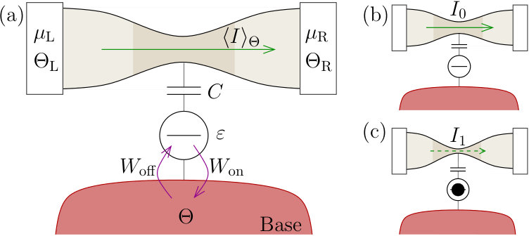 Figure 1
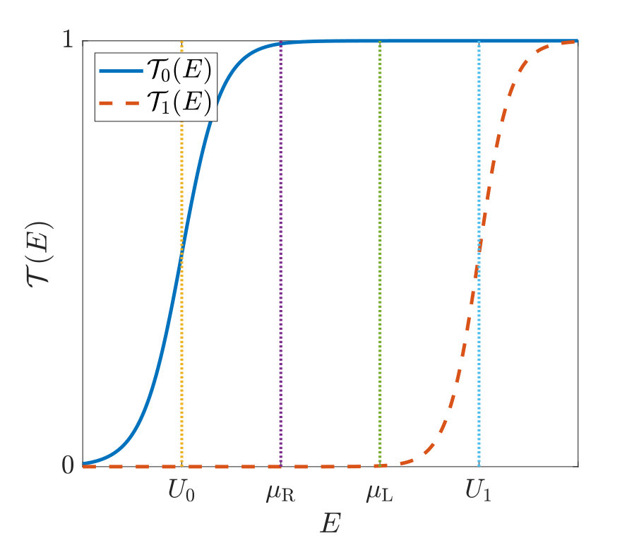 Figure 2
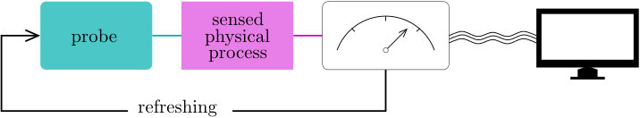 Figure 3
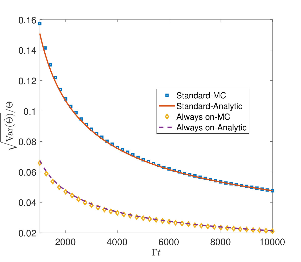 Figure 4
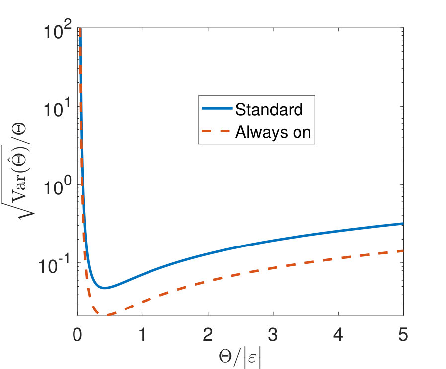 Figure 5
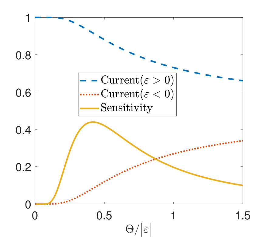 Figure 6
Peer Reviews
No public reviews on file for this paper yet. If you reviewed it on a platform where reviews are public (OpenReview, ICLR, NeurIPS, ICML), you can paste yours below so the community can read it here.
Videos
No videos yet. Explain this paper in a talk, walkthrough, or lecture? Add one.
Thermal transistor and thermometer based on Coulomb-coupled conductors
Jing Yang
Department of Physics and Astronomy, University of Rochester, Rochester, New York 14627, USA
Cyril Elouard
Department of Physics and Astronomy, University of Rochester, Rochester, New York 14627, USA
Janine Splettstoesser
Department of Microtechnology and Nanoscience (MC2), Chalmers University of Technology, S-412 96 Göteborg, Sweden
Björn Sothmann
Theoretische Physik, Universität Duisburg-Essen and CENIDE, D-47048 Duisburg, Germany
Rafael Sánchez
Departamento de Física Teórica de la Materia Condensada and Condensed Matter Physics Center (IFIMAC), Universidad Autónoma de Madrid, 28049 Madrid, Spain
Andrew N. Jordan
Department of Physics and Astronomy, University of Rochester, Rochester, New York 14627, USA
Institute for Quantum Studies, Chapman University, 1 University Drive, Orange, CA 92866, USA
Abstract
We study a three-terminal setup consisting of a single-level quantum dot capacitively coupled to a quantum point contact. The point contact connects to a source and drain reservoirs while the quantum dot is coupled to a single base reservoir. This setup has been used to implement a noninvasive, nanoscale thermometer for the bath reservoir by detecting the current in the quantum point contact. Here, we demonstrate that the device can also be operated as a thermal transistor where the average (charge and heat) current through the quantum point contact is controlled via the temperature of the base reservoir. We characterize the performances of this device both as a transistor and a thermometer, and derive the operating condition maximizing their respective sensitivities. The present analysis is useful for the control of charge and heat flow and high precision thermometry at the nanoscale.
I Introduction
Engineering and controlling heat and its coupling with electricity at the nanoscale is one of the big challenges that the field of nanoelectronics is facing today. The phenomenon of thermoelectric transport at the mesoscopic level has been widely explored in nanostructures to achieve this goal Sothmann et al. (2015); Benenti et al. (2017). This includes the design of nanoscale heat engines Staring et al. (1993); Dzurak et al. (1993); Humphrey et al. (2002); Entin-Wohlman et al. (2010); Sánchez and Büttiker (2011); Sothmann et al. (2012); Sothmann and Büttiker (2012); Bergenfeldt et al. (2014); Sánchez et al. (2015a); Hofer and Sothmann (2015); Roche et al. (2015); Hartmann et al. (2015); Thierschmann et al. (2015a); Whitney et al. (2016); Schulenborg et al. (2017); Josefsson et al. (2018); Sánchez et al. (2018), refrigerators Giazotto et al. (2006); Pekola and Hekking (2007); Edwards et al. (1993); Prance et al. (2009); Zhang et al. (2015); Koski et al. (2015); Hofer et al. (2016); Sánchez (2017), thermal rectifiers Scheibner et al. (2008); Ruokola and Ojanen (2011); Fornieri et al. (2014); Jiang et al. (2015); Sánchez et al. (2015b); Martínez-Pérez et al. (2015), and thermal transistors Li et al. (2006); Jiang et al. (2015); Joulain et al. (2016); Sánchez et al. (2017a, b); Zhang et al. (2018); Tang et al. (2019); Guo et al. (2018). Also the detection of heat flows in such devices via nanoscale low-temperature thermometers Correa et al. (2015); Hofer et al. (2017); Mehboudi et al. (2018); De Pasquale and Stace (2018) has been addressed. Remarkable progress has been recently achieved with different mesoscopic devices for milikelvin Spietz et al. (2003, 2006); Gasparinetti et al. (2011); Mavalankar et al. (2013); Feshchenko et al. (2013); Maradan et al. (2014); Feshchenko et al. (2015); Iftikhar et al. (2016); Ahmed et al. (2018); Karimi and Pekola (2018); Halbertal et al. (2016) or ultrafast Zgirski et al. (2018); Wang et al. (2018); Brange et al. (2018) thermometry.
Recent interest has been raised in designing multiterminal devices able to separate charge and heat currents. Proposals include the use of three terminal configurations of capacitively coupled quantum dots where transport through two (source and drain) terminals responds to charge fluctuations in the third one (the base), involving heat but no charge transfer. Setups of this kind allow for the realization of heat engines Sánchez and Büttiker (2011); Sothmann et al. (2012); Roche et al. (2015); Hartmann et al. (2015); Thierschmann et al. (2015a); Whitney et al. (2016); Daré and Lombardo (2017); Walldorf et al. (2017); Strasberg et al. (2018), refrigerators Zhang et al. (2015); Koski et al. (2015); Sánchez (2017); Erdman et al. (2018), thermal transistors Thierschmann et al. (2015b); Sánchez et al. (2017a, b); Zhang et al. (2018) and thermometers Zhang and Chen (2018). Of particular interest is the case of thermal transistors and non-invasive thermometers, where one seeks to maximize the response of the system (a current from source to drain) by minimizing the injection of heat from the base terminal. In the first case, transport in the system is modulated by changes in the base temperature, . Conversely in the second case, the current serves as readout of the temperature of the base. However, the tunneling current through a weakly-coupled quantum dot (based on single-electron transitions) is small.
To overcome this issue, we consider an alternative structure, shown in Fig. 1, consisting of a capacitively coupled quantum dot and a quantum point contact (QPC). The quantum dot is tunnel coupled to the base reservoir, which has a given temperature . The steady-state population of the quantum dot impacts the average (charge and heat) currents through the QPC, which in turn is connected to source and drain reservoirs. This structure has been employed previously to study the full counting statistics of single electron transport in quantum dots both theoretically Korotkov (1999, 2001, 2003); Pilgram and Büttiker (2002); Jordan and Büttiker (2005a, b); Jordan and Korotkov (2006); Jordan et al. (2006); Sukhorukov et al. (2007); Flindt et al. (2009) and experimentally Gustavsson et al. (2006); Fujisawa et al. (2006); Ubbelohde et al. (2012); Küng et al. (2012); Hofmann et al. (2016a, b); Entin-Wohlman et al. (2017), where the QPC acts as a charge detector that monitors the occupation of the dot. This setup was also experimentally demonstrated Gasparinetti et al. (2012); Torresani et al. (2013); Mavalankar et al. (2013); Maradan et al. (2014) to behave as a thermometer, enabled by the fact that the population of the dot is sensitive to the temperature in the base reservoir.
In this paper, we show that the structure can be used as a thermal transistor as well. We analyze its performance both as a transistor and a thermometer by deriving the corresponding sensitivities and finding the operating conditions optimizing them. When the device is operated as a thermal transistor, the goal is that a small temperature change in the base reservoir triggers a large change of the average charge or heat current in the QPC. We quantify the device performance by the differential sensitivity of the average charge and heat current to the infinitesimal temperature change in the base, as well as by the power gain.
For the operation of the device as a thermometer, we apply metrological tools to characterize two measurement protocols. The first one involves the sequential coupling to the dot to the probed reservoir and the QPC. This corresponds to the paradigmatic protocol of classical and quantum metrology Giovannetti et al. (2011). In the second protocol, both interactions are always turned on. This latter procedure is easier to implement and was actually used in Refs. Gasparinetti et al. (2012); Torresani et al. (2013); Mavalankar et al. (2013); Maradan et al. (2014). Both protocols allow noninvasive temperature measurements since single electron tunneling only involves a very small amount of energy and charge exchange between the measured reservoir (the base) and part of the thermometer (the quantum dot). When optimally operated, we find that the thermometer’s sensitivity is for both protocols limited by telegraph noise induced in the QPC by electron tunneling in the dot. Interestingly, the optimal sensitivity of the thermometer occurs for the same quantum-dot parameters as the optimal sensitivity of the thermal transistor. In contrast to the thermal transistor, we find that the sensitivity limits of the thermometer do not depend on the QPC current in the two quantum-dot charge configurations. For the thermal transistor, instead, we find that the power gain is independent of the dot occupation and the base-reservoir temperature.
With respect to the previously studied setup containing two capacitively coupled dots, the device shown in Fig. 1 has two definite advantages. First, the average currents flowing through the QPC are much larger than in the quantum-dot case where the Coulomb-blockade much reduces the conductance compared to the conductance quantum Nazarov and Blanter (2009). Furthermore, backaction is suppressed: In a QPC, there is no significant charge-buildup in the vicinity of the saddle point potential, which forms the QPC. As a consequence, the quantum dot state modifies the transmission probability of the QPC without energy exchange between the quantum dot and the QPC. This property allows to obtain high power gain for the transistor and participates to make the thermometer noninvasive as only a small bounded amount of energy flows back and forth between the dot and the base without involving the QPC. This situation is different for transport through a quantum dot connecting source and drain lead. In the latter case, random fluctuations of the electrostatic potential caused by the nearby, capacitively coupled gate dot Sánchez et al. (2017b, a) (or simply environmental fluctuations Sothmann et al. (2012); Ruokola and Ojanen (2012); Rosselló et al. (2017); Entin-Wohlman et al. (2017)) do induce energy exchange between the source-drain system and the base part in general. Exceptions have been identified involving particular tunneling rate configurations or strongly coupled dots Sánchez et al. (2017b, a).
The paper is organized as follows. In Sec. II we introduce the model of our setup. The operation as a thermal transistor is discussed in Sec. III while the thermometer configuration is analyzed in Sec. IV. Our results are summarized and conclusions are drawn in Sec. V.
II Setup
We consider a three-terminal device as shown in Fig. 1. It contains a spinless single-level quantum dot, which can be either empty, denoted as [math], or occupied with a single electron, denoted as (this corresponds to a quantum dot in the spin-split Coulomb-blockaded regime). The addition energy is defined as the energy difference of these two states. The dot is weakly tunnel coupled to the base reservoir with chemical potential and temperature . In what follows we choose the electrochemical potential of the base reservoir as a reference energy, . Throughout this article, we set . The coupling strength between dot and base reservoir is characterized by the rate . The population dynamics of the weakly coupled dot, with is described by the rate equations
[TABLE]
and , where and denote the probability to find the dot empty or singly occupied at time , respectively. According to Fermi’s golden rule, the transition rate from dot state [math] to is and the transition rate from dot state to [math] is where is the Fermi function. The dot occupations relax to the steady state on a time scale . The steady state populations are
[TABLE]
The mesoscopic QPC is connected to two macroscopic source and drain reservoirs with electrochemical potentials and temperatures , and , respectively, as shown in Fig. 1. The average current in the QPC sensitively depends on the state of the nearby quantum dot due to Coulomb interactions. For an ideal, saddle shaped potential landscape where transport occurs only via the lowest transverse mode, the QPC transmission takes the form Büttiker (1990)
[TABLE]
Here represents the empty or occupied state of the dot, characterizes the curvature of the potential, and is the electrostatic potential at the bottom of the saddle point when the dot is empty or occupied. In the nonlinear transport regime, it is important to account for the dependence of on the electrochemical potentials of the leads, with , to ensure gauge invariance Christen and Büttiker (1996). Throughout this paper, we assume that is much smaller than all relevant energy scales in the QPC subsystem, in particular, and , so that can be approximated by the Heaviside function. Then the energy relevant to electronic and heat transport falls in the range . The average charge and heat currents flowing out of a reservoir, for a given dot state, can be calculated from the Landauer-Büttiker formula Datta (1997); Blanter and Büttiker (2000). Focusing on currents flowing out of the left reservoir, we find
[TABLE]
[TABLE]
where for simplicity, we have chosen not to indicate the reservoir L, where we always assume currents to be detected. The subscript stands for the dot state. Given the dot stays in state , the current noise in the QPC is fully characterized by shot noise. Since we assume the low-temperature limit, thermal noise can be neglected. The zero frequency shot noise power spectral density of the charge current—considering auto-correlations in reservoir L—is Blanter and Büttiker (2000)
[TABLE]
where, again, the subscript indicates the dot state.
III Thermal transistor
III.1 Sensitivity
When the device under study acts as a thermal transistor in the steady state, analogous to the electric transistor, we would like to see a large change of average charge or heat current in the QPC due to a small change in the temperature of the base reservoir. Control of charge and heat currents via temperature gradients can be useful if, e.g., a certain device operation should only be performed as long as a certain temperature is not exceeded.
When the dot reaches its stationary state at a given base-reservoir temperature , the average charge current flowing in the QPC is
[TABLE]
where
[TABLE]
For the average heat current one just needs to replace , and with , and \Delta I^{Q}\equiv\big{|}\langle I_{0}^{Q}\rangle-\langle I_{1}^{Q}\rangle\big{|} respectively. We see from Eq. (8) that both the steady-state average charge and heat current depend on the temperature of the base reservoir through the steady-state population of the dot. The differential sensitivity of the average charge current in the QPC to the temperature of the base reservoir is111Note that we exclude the case , where the device is fully insensitive to temperature changes.
[TABLE]
where we have introduced the function for the normalized differential sensitivity
[TABLE]
We observe that the asymmetric function reaches its maximum at \big{|}x\big{|}=2.4 and decreases to half of its value at \big{|}x\big{|}=1 and \big{|}x\big{|}=4.5. Thus for fixed , the prefactor on the right hand side of Eq. (10) reaches its maximum at \Theta\approx 0.4\big{|}\varepsilon\big{|}, with left width 0.2\big{|}\varepsilon\big{|} and right width 0.6\big{|}\varepsilon\big{|}, as shown in Fig. 2. From this, we derive the maximum differential sensitivity as
[TABLE]
For the differential sensitivity of the average heat current, one just needs to replace in Eqs. (10, 12) with .
III.2 Power gain
In general, the power gain of a transistor is defined as the ratio between output and input power . Here, the output power is given by the power difference as the temperature is changed from to at a given applied voltage , i.e.,
[TABLE]
The definition of the input power is less straightforward, since within the considered model no energy flows from the quantum dot into the QPC circuit. Instead, the relevant energy flow is here the energy transferred from the base reservoir into the quantum dot within a time duration set by the characteristic time scale of the quantum-dot tunneling dynamics, when the reservoir temperature is changed from an initial value to a final value . Therefore, we find
[TABLE]
With this the result for the power gain is found to be
[TABLE]
Interestingly, the information about the occupation of the dot and about the temperature of the base reservoir drops out.
For fixed applied bias , one can further maximize the sensitivity, Eq. (12), and the power gain, Eq. (15), over or . It is readily found from Eqs. (5) and (6) that the maxima of both quantities are reached when the different dot occupations (empty or occupied) result into a completely closed or open QPC channel, corresponding to and respectively. This regime can be reached by tuning the parameters and such that one has and as shown in Fig. 3. In this regime, we have , but , and .
IV Thermometer
We now turn to the operation of the setup as a thermometer. We analyze two different types of protocols with the aim to sense the temperature of the base reservoir. The standard protocol of metrology, shown in Fig. 4 and described in detail in the figure caption, corresponds to a sequence of discrete measurements: a physical system (the quantum dot, in our case) is used as a probe which is prepared in some known initial state and then undergoes some physical process (charging/uncharging) which depends on the true value of the estimation parameter of interest (the temperature of the base reservoir, ). In this way, the information about the estimation parameter is encoded in the state of the probe. Finally, one uses some measuring apparatus (the QPC) to measure the state of the probe. When repeating the above procedure times, the standard precision of the measurement scales as . An alternative but more practical protocol (this is the one actually used in experiments Refs. Mavalankar et al. (2013); Maradan et al. (2014)) is to keep both interactions always on, avoiding the sequential coupling and decoupling procedures.
The QPC as a measurement apparatus or detector of the state of the dot has been widely discussed in the context of mesoscopic measurement processes Korotkov (1999, 2001, 2003); Pilgram and Büttiker (2002); Jordan and Büttiker (2005a, b); Jordan and Korotkov (2006); Jordan et al. (2006); Sukhorukov et al. (2007); Flindt et al. (2009); Gustavsson et al. (2006); Fujisawa et al. (2006); Ubbelohde et al. (2012); Küng et al. (2012); Hofmann et al. (2016a, b); Entin-Wohlman et al. (2017). Let us first for simplicity assume that the quantum dot is fixed to be either empty or filled, and that we want to determine the state of the dot by looking at the current flowing in the QPC. Although the on and off states of the dot correspond to different average current and in the QPC, we can not resolve these two current levels instantaneously, due to the shot noise. Therefore, to measure the state of the dot, one has to switch on the QPC circuit for some time duration. Suppose we measure for this time duration , which is much longer than the correlation time of the shot noise in the QPC and in principle depends on the dot state . Due to the central limit theorem, the distribution of the time average current conditioned on the dot state is a Gaussian with mean and variance , where is the zero frequency conditioned shot noise spectral density defined in Eq. (7). To reach a signal to noise ratio of at least unity for distinguishing the two Gaussians, the measurement must be turned on for at least a time duration of , where is defined in Eq. (9) and
[TABLE]
is the measurement time. If the QPC circuit is switched on for a time duration much longer than , it effectively performs an ideal measurement of the quantum-dot occupation.
IV.1 Standard (discrete) protocol
We now discuss the three steps of the protocol of Fig. 4. Therefore, (i) we initially prepare the quantum dot—the probe of our setup—in state [math], meaning that no excess electrons are in the dot. Next, (ii) we turn on the interaction with the base reservoir for a time duration , where the constant is sufficiently large to guarantee that the dot reaches the stationary state. We then (iii) turn off the interaction with the base reservoir and at the same time turn on the measurement by the QPC to determine whether there is an electron on the dot or not. We measure for time duration to perform an effectively noiseless ideal occupation measurement, where is chosen to obtain a sufficiently large signal-to-noise ratio here. The measurement gives a binary outcome statistically described by the probability mass function , Eqs. (2,3), corresponding to the two outcomes . The corresponding sensitivity of the measurement about the temperature associated with a single cycle is quantified by the Fisher information, which is given by
[TABLE]
Note that the inverse of the Fisher information sets the lower bound of the variance of any temperature estimator, known as the Cramér-Rao bound Kay (1993).
In a given time , one can repeat the cycle times. We denote the measurement outcome for the -th cycle as , where if the dot is empty and if the dot is occupied. Based on a series of measurement outcomes , we propose to apply the asymptotically unbiased maximum likelihood estimator to estimate the temperature, where . When is sufficiently large, the maximum likelihood estimator can saturate the Cramér-Rao bound asymptotically Kay (1993), which is given by
[TABLE]
For simplicity, we here assumed . In a typical experiment, one can resolve the state of the dot in a time scale much shorter than the life time of the state limited by electron tunneling. This indicates that the time scale of the tunneling is much longer than the time scale required to resolve the two current levels, . With this approximation, Eq. (18) reduces to
[TABLE]
which is independent of the QPC parameters. Now, from the property of the function discussed in Sec. III, we see that
[TABLE]
and the variance ranges between the minimum variance when \big{|}\varepsilon\big{|} is tuned between . Equation (20) is confirmed by Monte Carlo simulation as shown in Fig. 5, where we generate the noiseless measurement signals (electric current) in the QPC according to the probability mass function described by Eq. (1). The simulation shows that one needs to take in order to obtain a numerical variance (square markers) of the maximum likelihood estimator, which approaches the Cramér-Rao bound (20) (red solid line) in the long time limit.
Since the optimal value of \big{|}\varepsilon\big{|} depends on the true value of the estimated temperature, the maximum sensitivity given by Eq. (20) can only be reached by adaptive measurements consisting of multiple rounds, where one needs to adjust the value of \big{|}\varepsilon\big{|} according to the temperature estimate from the previous round. If \big{|}\varepsilon\big{|} is kept fixed all the time, as shown in Fig. 6, the normalized standard deviation of the temperature estimator diverges exponentially at low temperature and linearly at high temperature.
IV.2 Always-on estimation
Let us now consider the alternative protocol, where the measurement by the QPC and the interaction with the electron reservoir are always turned on. We estimate the temperature of the base reservoir using the transferred charge in the QPC. When the dot reaches its steady state, the average current in the QPC is described by Eq. (8), where the impact of the quantum dot enters via its steady-state occupation probabilities. This QPC current has statistical fluctuations, which can be attributed to two different sources of noise. The first is the already mentioned shot noise, described by Eq. (7), due to the partially open channel in the QPC. The other source is telegraph noise, which stems from stochastic switching of the dot states caused by electrons tunneling on and off the quantum dot. We define the transferred charge in the QPC between the beginning of the measurement at up to time as
[TABLE]
The full counting statistics gives the cumulants of Levitov et al. (1996); Jordan and Sukhorukov (2004); Sukhorukov et al. (2007); Singh et al. (2016), see also Appendix A. The first and second cumulants of are
[TABLE]
[TABLE]
Now we estimate the occupation by some specific sampling of according to Eq. (22). This results in the following estimator
[TABLE]
This estimator has a simple physical interpretation: the occupation of the dot is estimated from the duration of time spent on the dot, divided by the total time of the experiment. Note that in the long time limit, the distribution of is approximately Gaussian. Then the occupation estimator (24) is also the maximum likelihood estimator. According to Eq. (22), it is an unbiased estimator, i.e., . The variance of such an estimator is
[TABLE]
For sufficiently long such that is small, we can calculate the variance of the temperature estimator through the following error propagation relation
[TABLE]
From Eq. (26), we find
[TABLE]
Direct minimization of Eq. (27) is tedious but can be done numerically. As in Sec. IV.1, we assume the practical situation to simplify the minimization. With this assumption, we see that as long as the detuning \big{|}\varepsilon\big{|} is not much larger than , such that is neither close to [math] nor , the contributions from the shot noise in Eq. (27) can be safely ignored. Therefore Eq. (27) reduces to
[TABLE]
which is independent of the QPC parameters as in the standard protocol. When is maximized at \big{|}\varepsilon\big{|}/\Theta=2.4, and consequently , the shot noise can be neglected as long as . In this case the minimum variance is
[TABLE]
Eq. (29) is confirmed by Monte Carlo simulation as shown in Fig. 5, where we simulate the telegraph process to generate the measurement signals in the QPC. As in the standard protocol, the optimal regime requires the knowledge of the true value of and therefore adaptive measurements are required in general. The behavior of the temperature estimator in a non-adaptive measurement is qualitatively the same as the standard protocol, as shown in Fig. 6. However, near the optimal regime the always-on protocol has a factor of 5 smaller variance than the standard protocol, as shown in Fig. 5.
V Conclusion
We have analyzed a setup consisting of a quantum dot capacitively coupled to a QPC as shown in Fig. 1 used as a nanoscale thermal transistor and noninvasive thermometer. The basic operation principle relies on the sensitivity of the average charge and heat current through the QPC to the average occupation of the quantum dot. The average dot occupation in turn depends on the temperature of the base reservoir. We characterized the performance of the thermal transistor by its power gain as well as the differential sensitivity of the average charge current through the QPC to a variation of the temperature of the base reservoir. The performance of the thermometer was characterized by the variance of the temperature estimator. Furthermore, the thermometer is noninvasive since reading out the temperature only involves single electron tunneling and it is assumed that there is no energy exchange between the base and the QPC .
Interestingly, as a consequence of the common operation principles, we have found that for both types of devices the maximal sensitivity occurs when the addition energy of the dot and the temperature of the base reservoir are related as . However, while for the transistor the base temperature is optimized at fixed addition energy, for the thermometer the optimization has to be performed over the addition energy keeping the base temperature fixed. Furthermore, while the sensitivity of the transistor depends on the difference of the average QPC currents, the sensitivity of the thermometer, characterized by the variance of the temperature estimator, is independent of .
The setup proposed here has already been implemented experimentally Gasparinetti et al. (2012); Torresani et al. (2013); Mavalankar et al. (2013); Maradan et al. (2014) for thermometers. Our work shows its interest for the purpose of controlling charge or heat flow at the nanoscale and sets its theoretical ideal performance.
Acknowledgements.
We thank the KITP for hosting the program Thermodynamics of Quantum Systems: Measurement, engines, and control, where this work was initiated. This research was supported in part by the National Science Foundation under Grant No. NSF PHY-1748958. JY, CE, and ANJ acknowledge the support from the U.S. Department of Energy, Office of Science, Office of Basic Energy Sciences under Award Number DE-SC-0017890 and the National Science Foundation under Grant No. NSF PHY-1748958. JS acknowledges funding from the Swedish VR and the Knut and Alice Wallenberg foundation through an Academy Fellowship. BS acknowledges financial support from the Ministry of Innovation NRW via the “Programm zur Förderung der Rückkehr des hochqualifizierten Forschungsnachwuchses aus dem Ausland”. RS acknowledges support from the Ramón y Cajal program RYC-2016-20778 and the “María de Maeztu” Programme for Units of Excellence in R&D (MDM-2014-0377).
Appendix A Full counting statistics of the transmitted charge
in the QPC
In this appendix we give a brief overview of the full counting statistics method applied to the current through the QPC, used in Sec. IV.2. We note that the statistical dependence of the transferred charges in consecutive time intervals, which are much larger than the typical correlation time of the current flowing in the QPC, can be neglected. Namely, for two consecutive time intervals , where , the charges transferred in the QPC denoted as and respectively can be treated as statistically independent. We define the total charge transferred during the two intervals as and denote the probability distributions of , and as , and respectively, where . Then is a convolution between and due to the statistical independence of and .
The moment and cumulant generating functions associated with are
[TABLE]
[TABLE]
Thus we have
[TABLE]
[TABLE]
As a consequence, the cumulant generating function of , where is defined in Eq. (21) takes the form
[TABLE]
We Taylor expand as
[TABLE]
and define
[TABLE]
Then, can be written as
[TABLE]
We denote the probability as the probability of transferring charge up to time and having the dot in state at time . We note that if there is no tunneling between the dot and the base reservoir,
[TABLE]
which is equivalent to writing the time-derivative as
[TABLE]
On top of this effect, we have to take into account the effect due to tunneling, which yields the master equation
[TABLE]
[TABLE]
Rewriting both sides in terms of the generation functions gives
[TABLE]
The above equation can be rewritten as
[TABLE]
where
[TABLE]
and
[TABLE]
Thus the solution to Eq. (44) is
[TABLE]
When is sufficient large, the unconditional cumulant generating function
[TABLE]
approaches the maximum eigenvalue of , which gives
[TABLE]
From this equation one can find
[TABLE]
[TABLE]
where \langle\!\langle I_{\alpha}\rangle\!\rangle=\partial H_{\alpha}(\lambda)/\partial\lambda\big{|}_{\lambda=0} and \langle\!\langle I_{\alpha}^{2}\rangle\!\rangle=\partial^{2}H_{\alpha}(\lambda)/\partial\lambda^{2}\big{|}_{\lambda=0} . In the long time limit, we can easily obtain
[TABLE]
and
[TABLE]
where , and are conditional average electric current in the QPC and the shot noise power spectral density defined in Eqs. (5, 7) respectively. With Eqs. (52, 53, 50, 51), one can easily obtain Eqs. (22, 23) in the main text.
The reference list from the paper itself. Each links out to its DOI / PubMed record.
- 1Sothmann et al. (2015) B. Sothmann, R. Sánchez, and A. N. Jordan, Nanotechnology 26 , 032001 (2015) . · doi ↗
- 2Benenti et al. (2017) G. Benenti, G. Casati, K. Saito, and R. Whitney, Phys. Rep. 694 , 1 (2017) . · doi ↗
- 3Staring et al. (1993) A. A. M. Staring, L. W. Molenkamp, B. W. Alphenaar, H. van Houten, O. J. A. Buyk, M. A. A. Mabesoone, C. W. J. Beenakker, and C. T. Foxon, Europhysics Letters (EPL) 22 , 57 (1993) . · doi ↗
- 4Dzurak et al. (1993) A. S. Dzurak, C. G. Smith, M. Pepper, D. A. Ritchie, J. E. F. Frost, G. A. C. Jones, and D. G. Hasko, Solid State Commun. 87 , 1145 (1993) . · doi ↗
- 5Humphrey et al. (2002) T. E. Humphrey, R. Newbury, R. P. Taylor, and H. Linke, Phys. Rev. Lett. 89 , 116801 (2002) . · doi ↗
- 6Entin-Wohlman et al. (2010) O. Entin-Wohlman, Y. Imry, and A. Aharony, Phys. Rev. B 82 , 115314 (2010) . · doi ↗
- 7Sánchez and Büttiker (2011) R. Sánchez and M. Büttiker, Phys. Rev. B 83 , 085428 (2011) . · doi ↗
- 8Sothmann et al. (2012) B. Sothmann, R. Sánchez, A. N. Jordan, and M. Büttiker, Phys. Rev. B 85 , 205301 (2012) . · doi ↗