Two-dimensional magnetohydrodynamic turbulence with large and small energy-injection length scales
Debarghya Banerjee, Rahul Pandit

TL;DR
This study compares two-dimensional magnetohydrodynamic turbulence driven at different scales, revealing distinct statistical behaviors, including energy equipartition and the prevalence of extreme events, through systematic numerical simulations.
Contribution
It provides a systematic comparison of 2D MHD turbulence at different forcing scales, highlighting differences in energy distribution and statistical properties.
Findings
Energy equipartition occurs at large-scale forcing.
Extreme events are more common at large-scale forcing.
Statistical properties differ significantly between the two forcing scales.
Abstract
Two-dimensional magnetohydrodynamics (2D MHD), forced at (a) large length scales or (b) small length scales, displays turbulent, but statistically steady, states with widely different statistical properties. We present a systematic, comparative study of these two cases (a) and (b) by using direct numerical simulations (DNSs). We find that, in case (a), there is energy equipartition between the magnetic and velocity fields, whereas, in case (b), such equipartition does not exist. By computing various probability distribution functions (PDFs), we show that case (a) displays extreme events that are much less common in case (b).
Click any figure to enlarge with its caption.
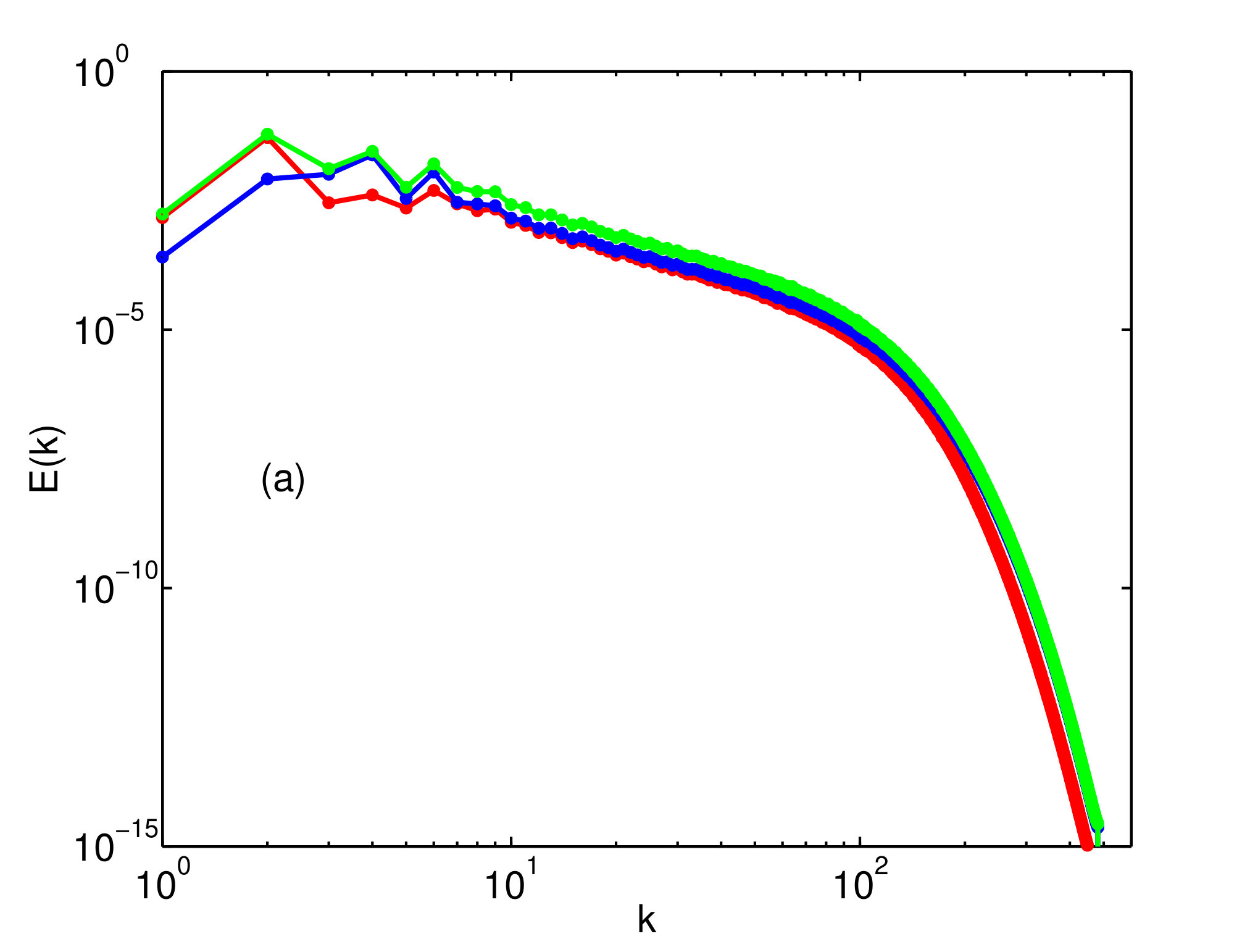 Figure 1
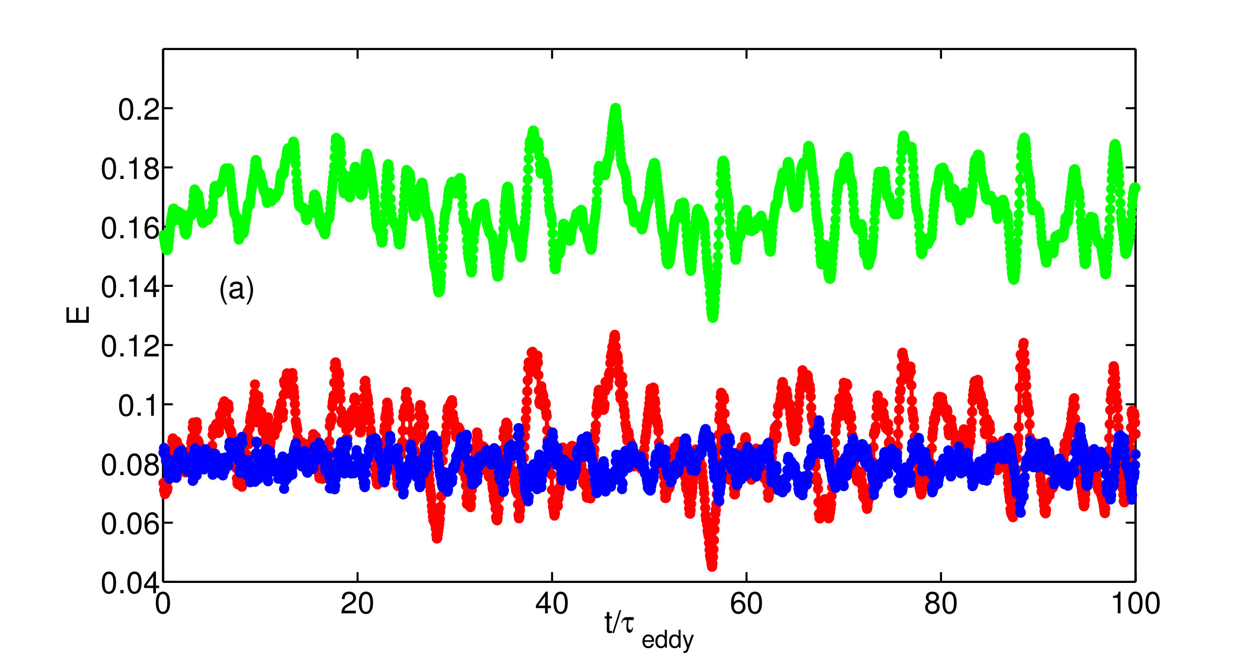 Figure 2
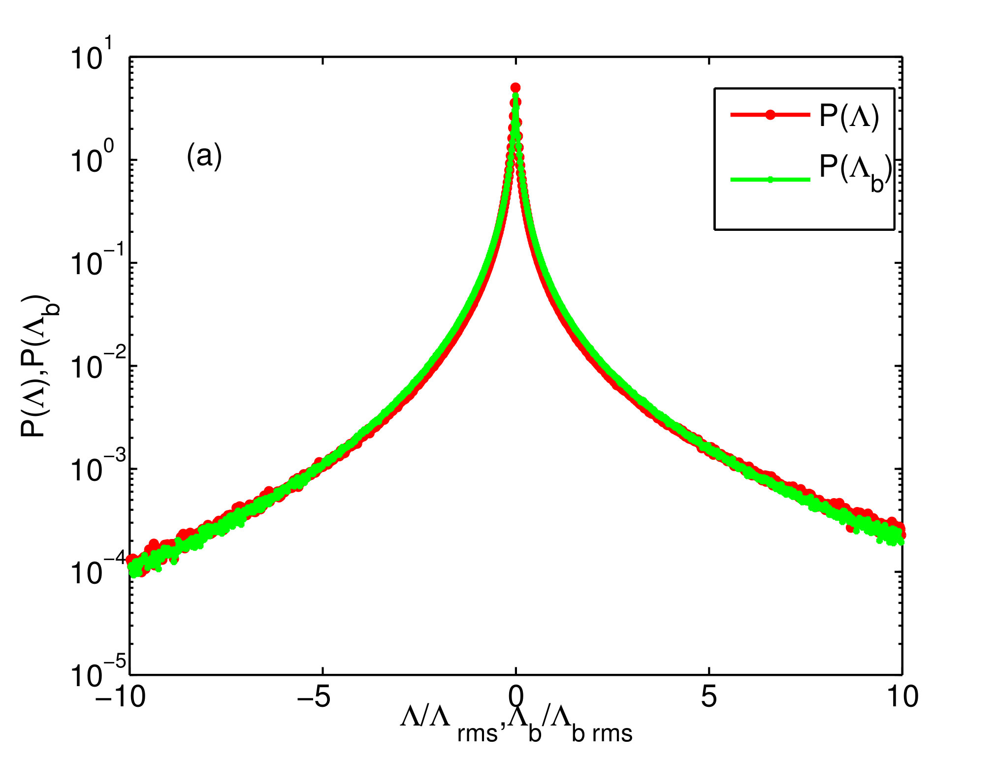 Figure 3
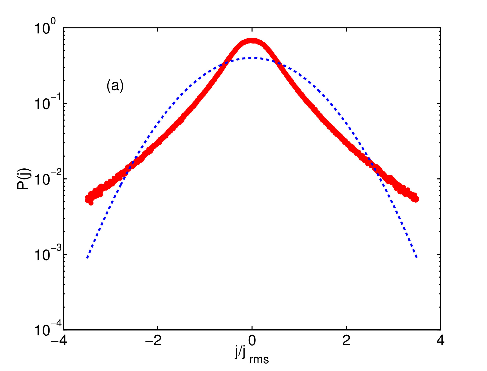 Figure 4
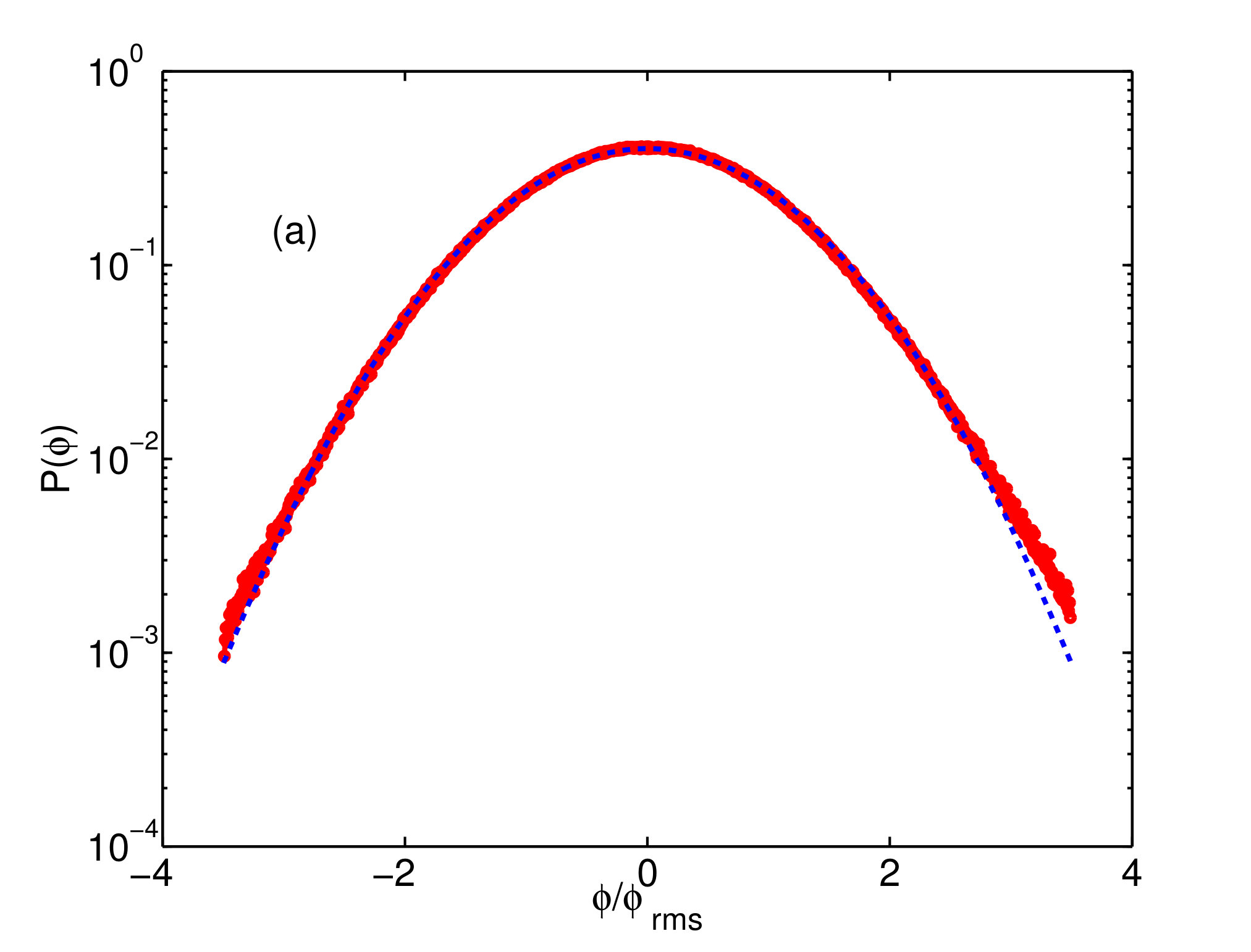 Figure 5
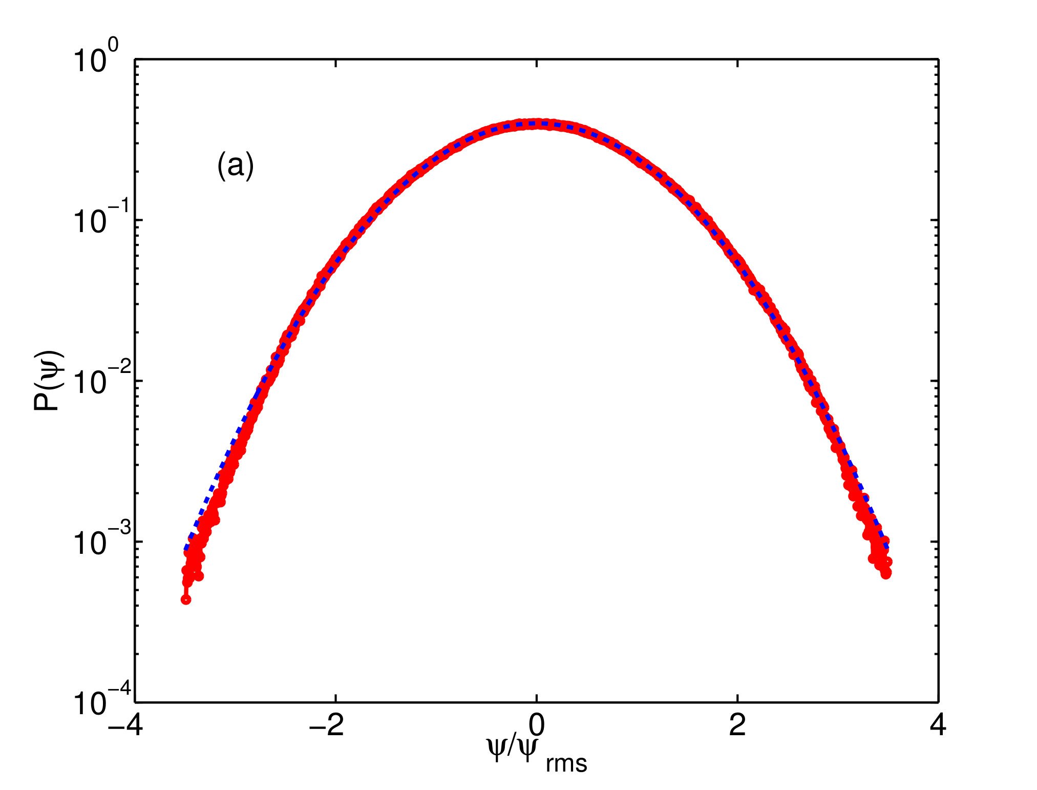 Figure 6
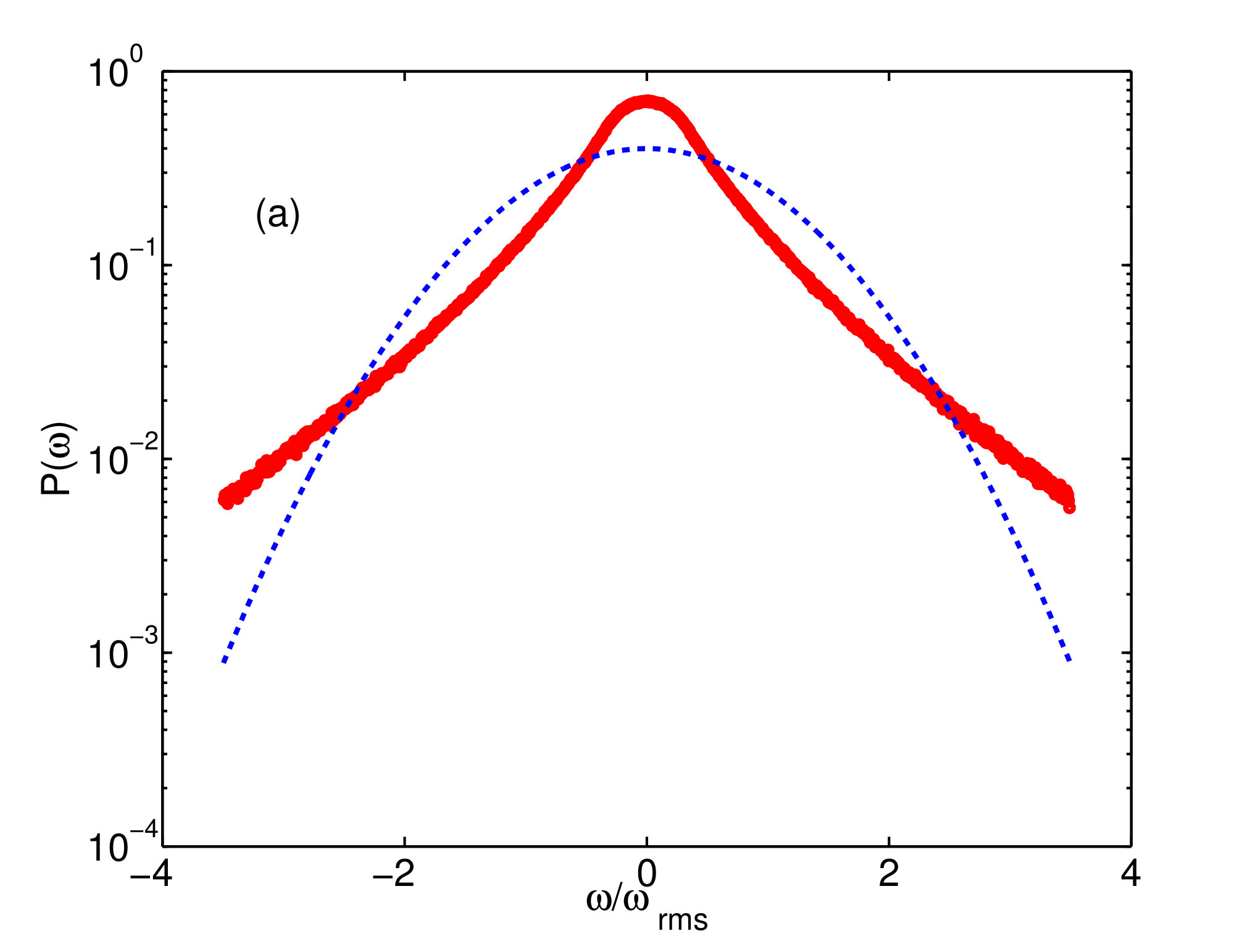 Figure 7
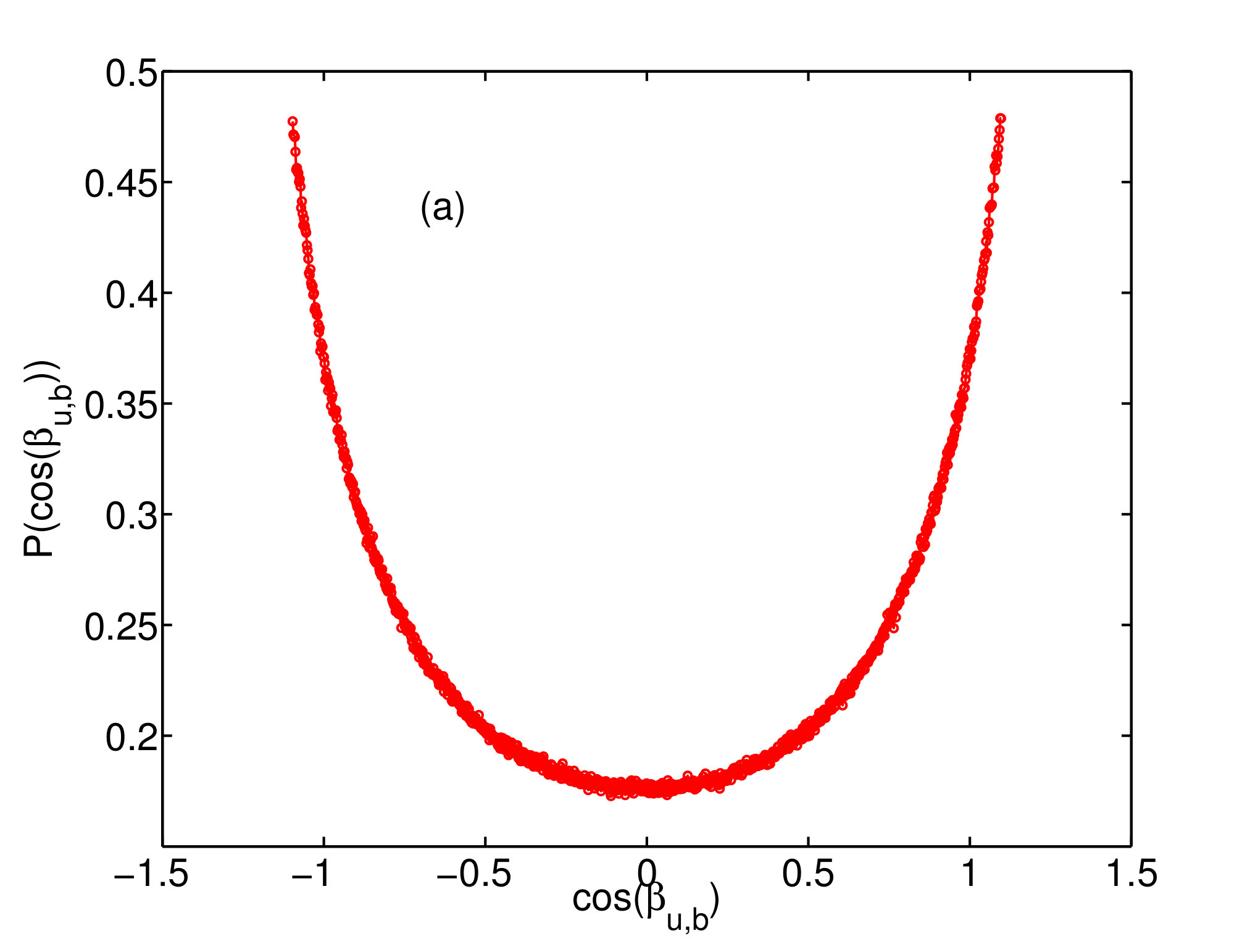 Figure 8
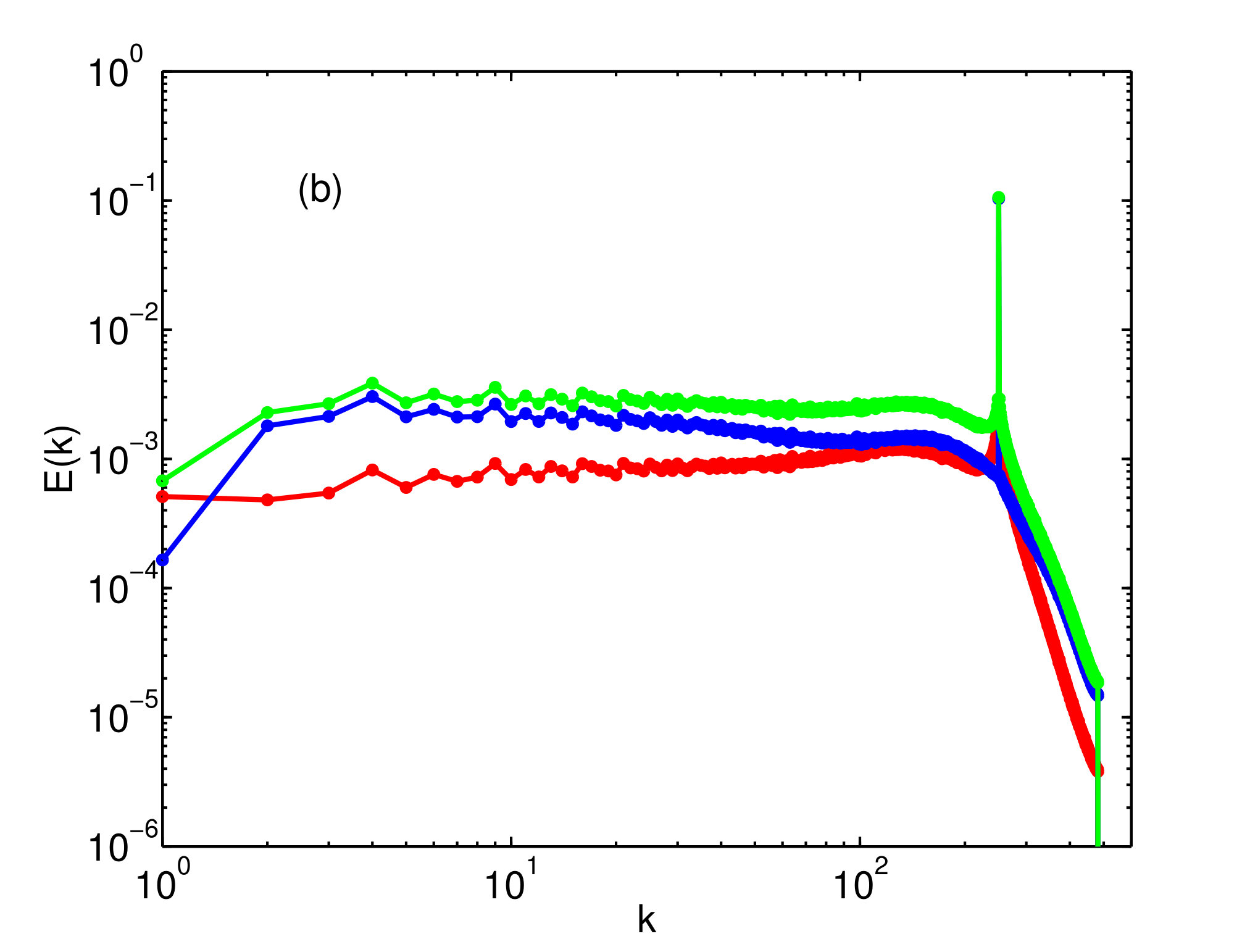 Figure 9
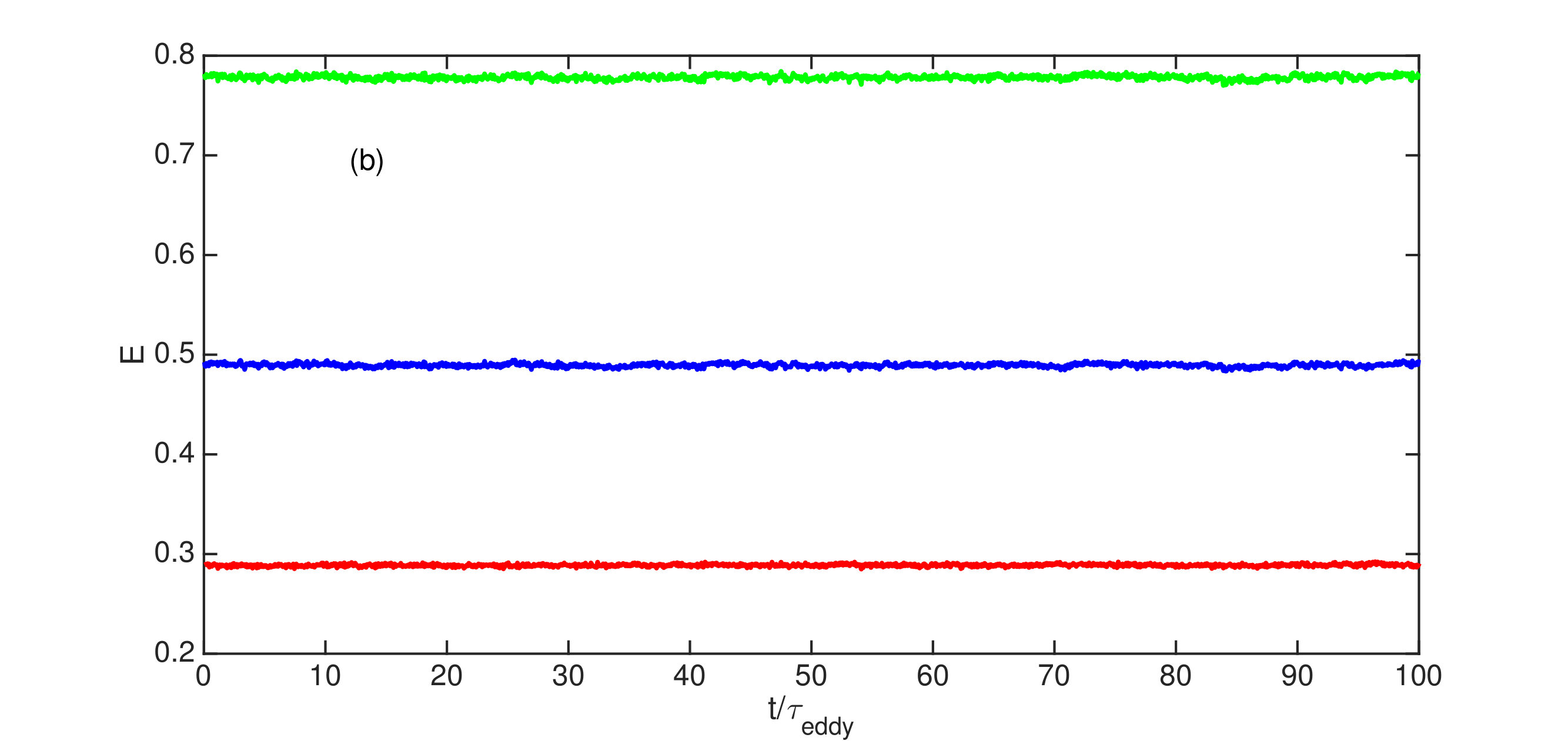 Figure 10
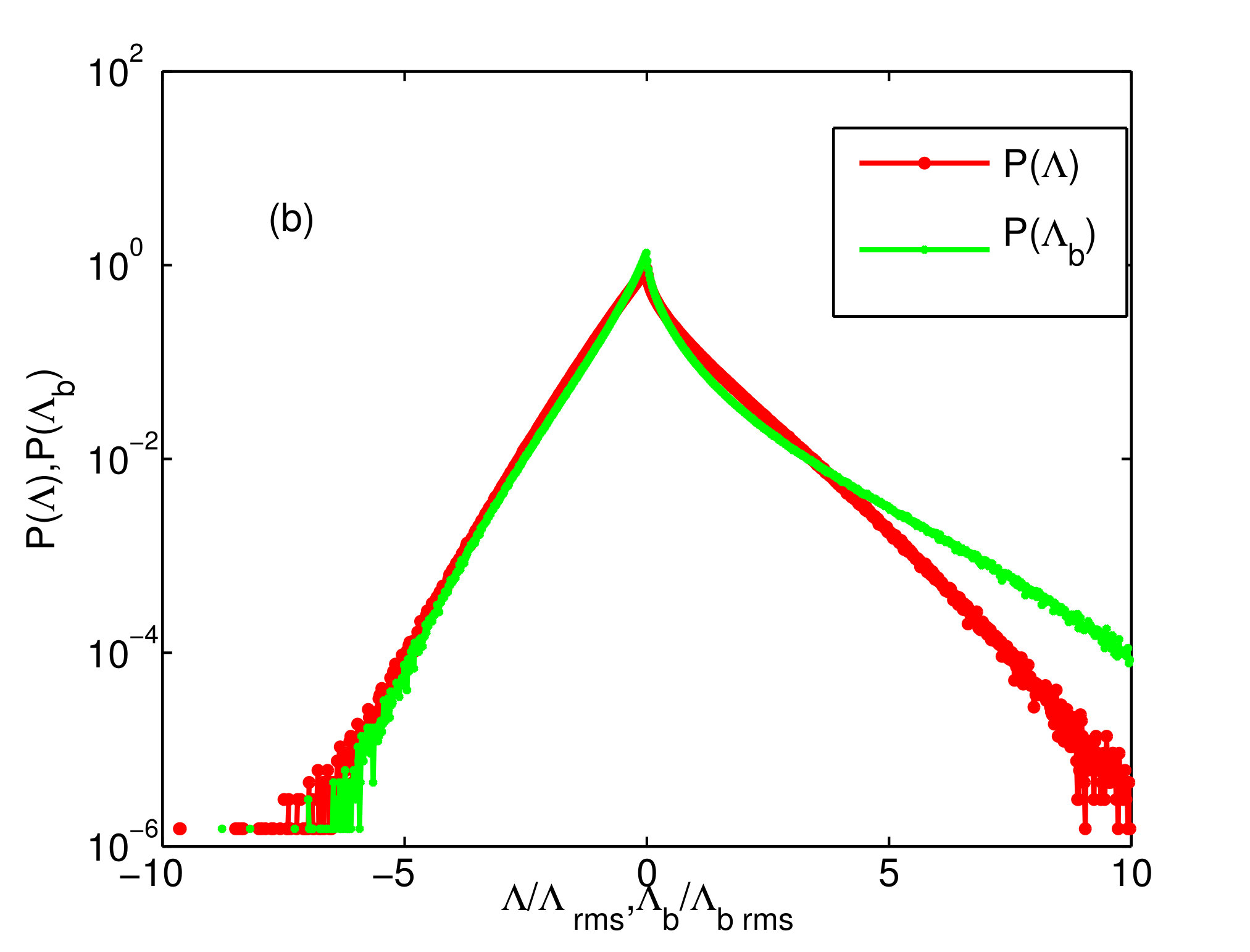 Figure 11
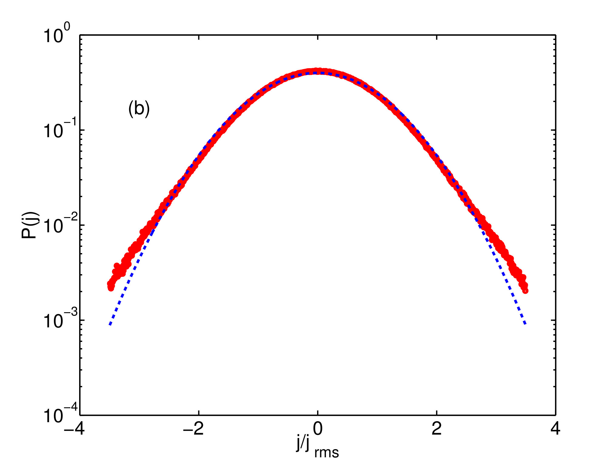 Figure 12
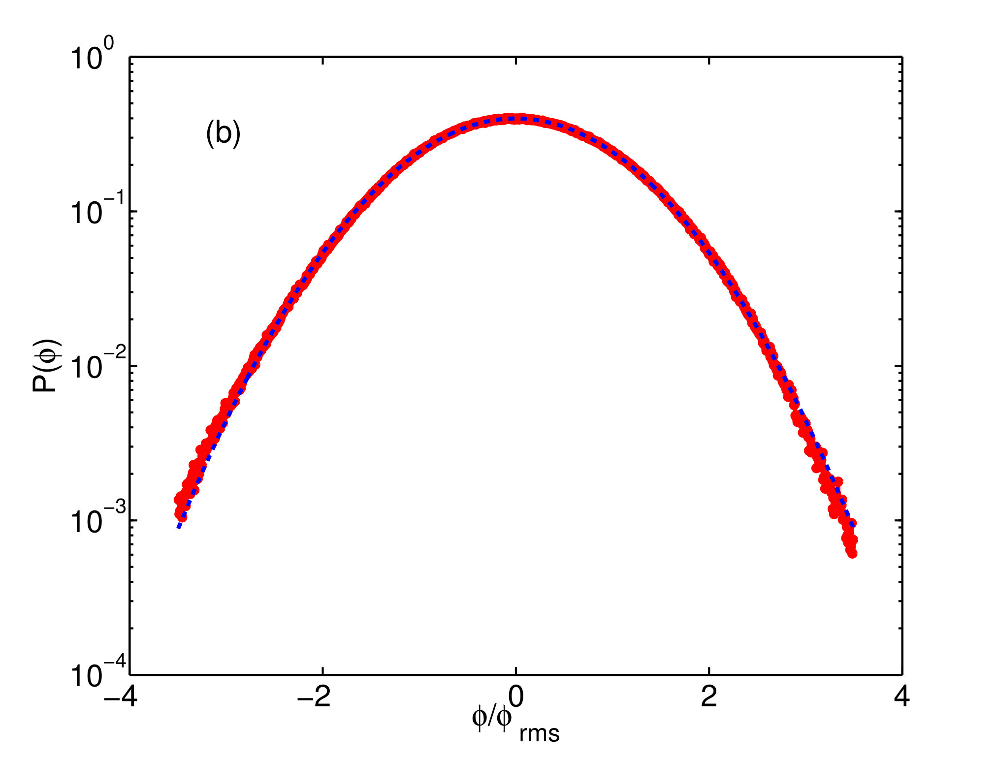 Figure 13
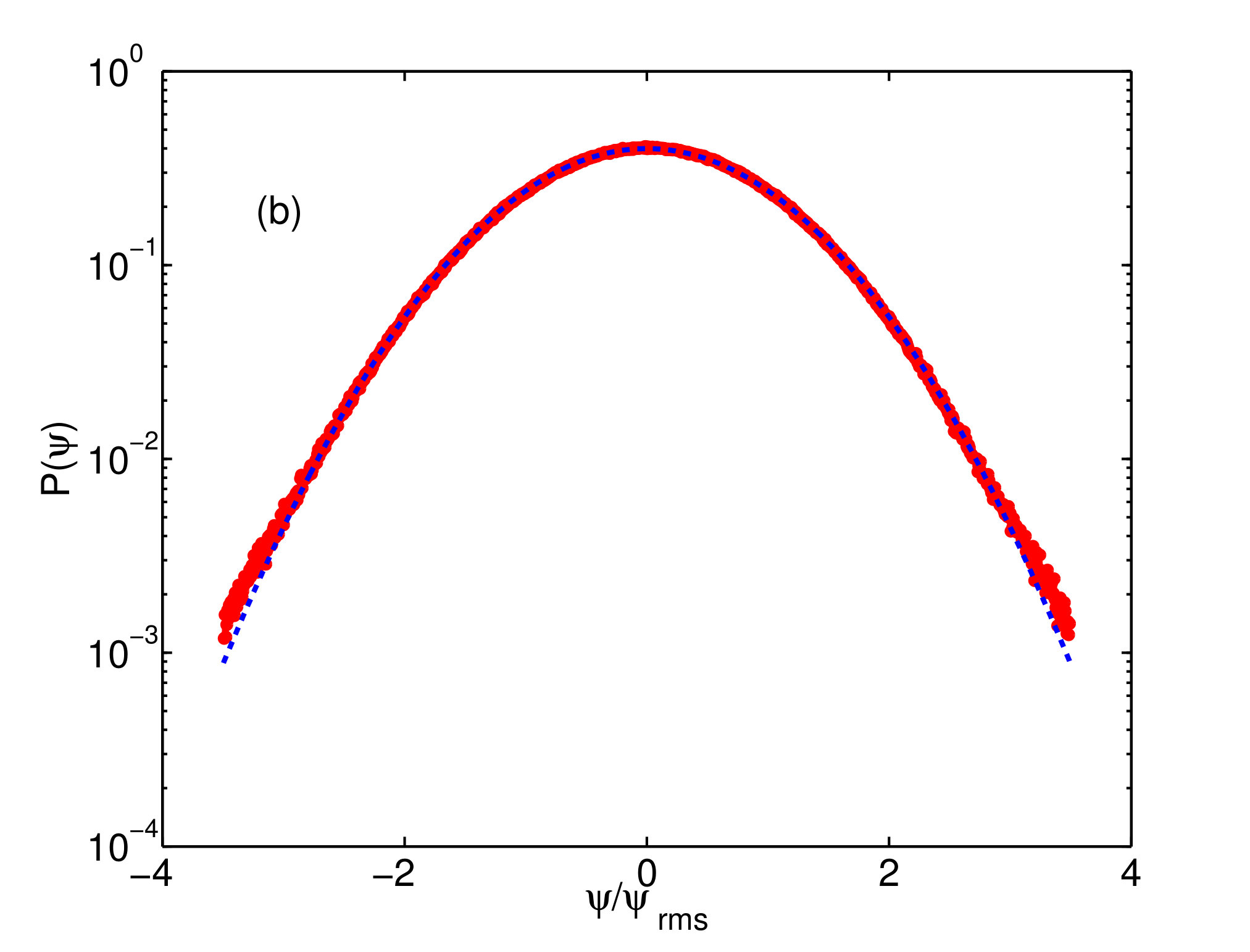 Figure 14
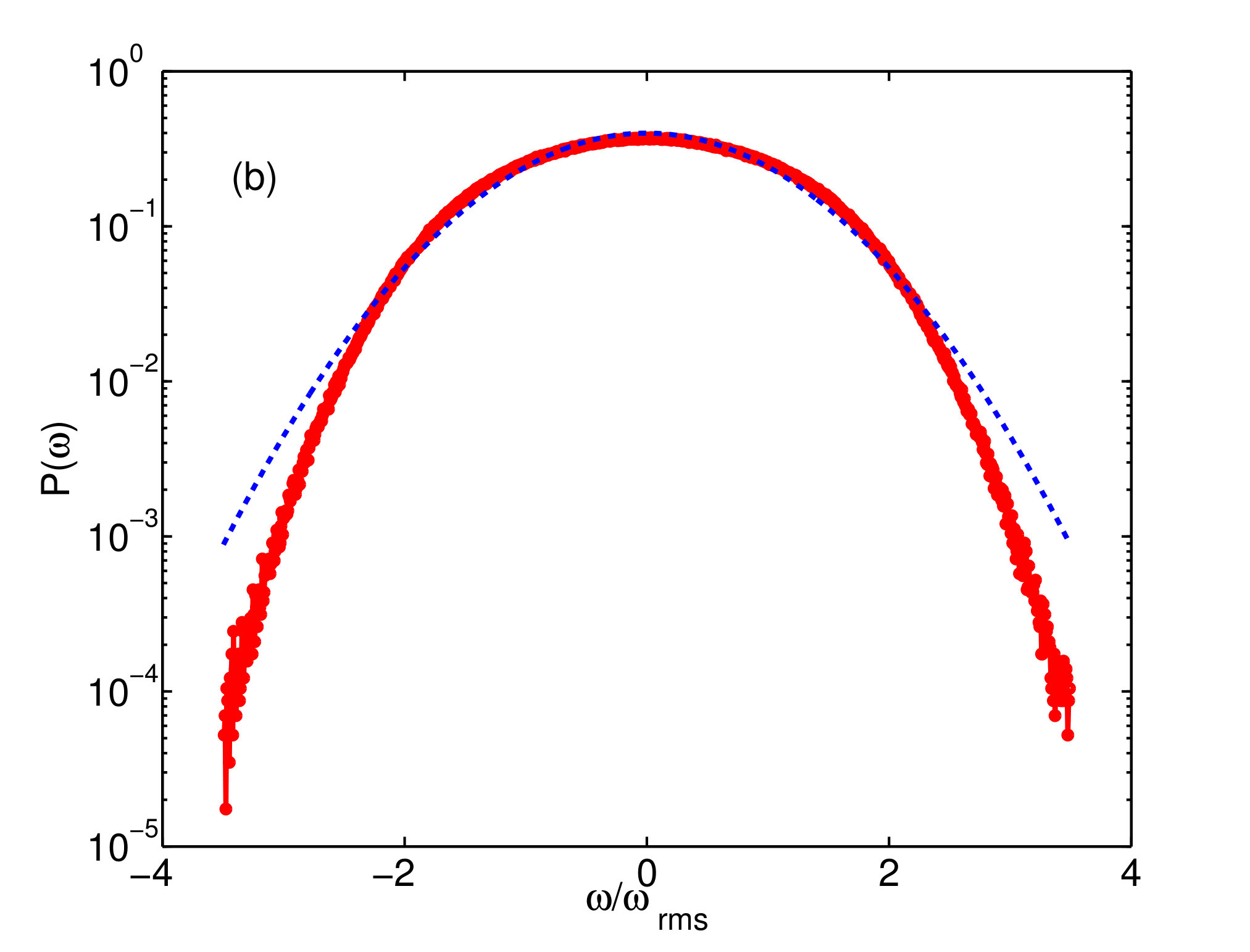 Figure 15
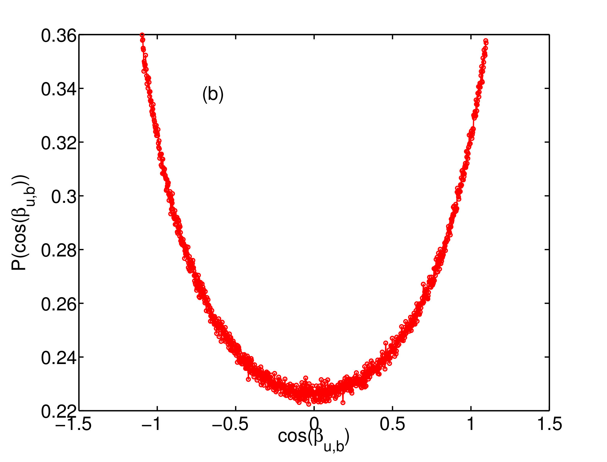 Figure 16
| Runs | |||||||||
|---|---|---|---|---|---|---|---|---|---|
| R1 | |||||||||
| R2 |
Peer Reviews
No public reviews on file for this paper yet. If you reviewed it on a platform where reviews are public (OpenReview, ICLR, NeurIPS, ICML), you can paste yours below so the community can read it here.
Videos
No videos yet. Explain this paper in a talk, walkthrough, or lecture? Add one.
Two-dimensional magnetohydrodynamic turbulence with large and small
energy-injection length scales
Debarghya Banerjee
Max Planck Institute for Dynamics and Self-Organization, Am Faßberg 17, 37077 Göttingen, Germany.
Rahul Pandit
Centre for Condensed Matter Theory, Department of Physics, Indian Institute of Science, Bangalore 560012, India.
Abstract
Two-dimensional magnetohydrodynamics (2D MHD), forced at (a) large length scales or (b) small length scales, displays turbulent, but statistically steady, states with widely different statistical properties. We present a systematic, comparative study of these two cases (a) and (b) by using direct numerical simulations (DNSs). We find that, in case (a), there is energy equipartition between the magnetic and velocity fields, whereas, in case (b), such equipartition does not exist. By computing various probability distribution functions (PDFs), we show that case (a) displays extreme events that are much less common in case (b).
I Introduction
Statistically steady turbulence, in fluids or magnetohydrodynamics (MHD), is sustained by external forcing. Away from boundaries and the scales at which energy is injected into the fluid, such turbulence is statistically homogeneous and isotropic. The length scale at which the external forcing acts determines, to a large extent, the nature and statistical properties of this turbulence Biskamp2003 ; Verma2004 . Nonlinear cascades of the energy or other quadratic invariants (e.g., the enstrophy , or the magnetic helicity , where and are, respectively, the velocity and magnetic fields, and is the magnetic vector potential) lead to different inertial ranges of length scales that lie between , the typical linear system size, and , the length scale at which dissipation becomes significant. In a turbulent fluid, the Fourier-space energy spectrum , where is the wave number and an exponent that characterizes this scaling form in the inertial range . In MHD turbulence, similar scaling forms hold for both the magnetic- and fluid-energy spectra Biskamp2003 ; Verma2004 and , respectively. Two-dimensional (2D) fluid turbulence displays two inertial ranges Frisch1995 ; Kraichnan1967 ; Fjortoft1953 ; Batchelor1969 ; Leith1972 : If the energy-injection or forcing length scale is , there are two scaling regimes in , namely, the forward-cascade regime, for , in which the enstrophy cascades from the forcing length scales towards the dissipation scale, and (b) the inverse-cascade regime, for , in which the energy goes from the injection length scale towards larger length scales Frisch1995 ; Kraichnan1967 ; Fjortoft1953 ; Batchelor1969 ; Leith1972 ; PanditOverview17 . In 2D MHD turbulence, 2D-fluid-turbulence-type arguments hold, but there is a forward cascade of energy and an inverse cascade of magnetic helicity Frisch1975 ; PanditOverview17 ; Banerjee2014 , if we assume that the cross helicity has a negligible effect on the dynamics. Other examples of inverse cascades can be found in turbulence in quasi-geostrophic flows Bistagnino2008 ; Bernard2007 , in rotating fluids Smith1999 , in fluid films with added polymers Gupta2015 , and in 3D MHD, which has an inverse cascade of magnetic helicity and forward cascades of the energy and cross helicity Alexakis2006 ; Biskamp2003 . By contrast, 3D fluid turbulence shows no inverse cascade, but only a forward cascade of energy.
The direction of cascades in turbulence can be predicted by using arguments of equilibrium statistical physics Kraichnan1980 . If we consider the invariants of the system to have a Gibbsian distribution, and we calculate the spectra of these invariants, then a maximum in the spectrum at small (large) indicates an inverse (forward) cascade. This was first shown, for 2D fluid turbulence, in the seminal work of Kraichnan Kraichnan1980 , who proposed the inverse-energy cascade, which implied the formation of large-scale vortical structures. These predictions Kraichnan1980 were based on arguments of equilibrium statistical physics Lee1952 applied to the 2D, Galerkin-truncated Euler equations, whose finite-dimensional phase space allowed the Galerkin-truncated system to thermalise to an equilibrium state. This statistical-mechanical technique has been used, subsequently, to predict the natures of cascades in a wide variety of turbulent systems Krstulovic2009 , including MHD turbulence: it has revealed the inverse cascades of (a) the magnetic helicity in 3D MHD turbulence and (b) the squared magnetic potential in 2D MHD turbulence Banerjee2014 . From the forward cascade of total energy ) and the inverse cascade of , and by using dimensional analysis, it is possible to predict the scaling forms of the energy spectrum in the forward- and inverse-cascade regimes Biskamp2003 in 2D MHD turbulence.
In Ref. Banerjee2014 , we have outlined the dimensional arguments that are used for extracting the scaling exponents in the inverse-cascade regime of 2D MHD turbulence. We give below similar arguments for the forward-cascade regime:
[TABLE]
here, we indicate by square brackets the dimensions of different quantities and express them as powers of length and time . (Recall that the velocity and magnetic fields have the same units in the standard formulation of MHD; and and are the dissipation rates of kinetic energy and magnetic energy, respectively.) We use the type of power-law Ansatz employed by Kolmogorov K41 in 1941 (K41) for 3D fluid turbulence, namely,
[TABLE]
by dimensional analysis we obtain
[TABLE]
and thence and , i.e.,
[TABLE]
Note that these dimensional and scaling arguments are predicated upon a K41-type phenomenology; strictly speaking this is not correct because of intermittency corrections that lead to multifractality Frisch1995 ; furthermore, these arguments do not account for a bottleneck in the energy spectrum at intermediate wavenumbers Frisch2008 ; Frisch2013 . For discussions of energy-spectral exponents in 3D MHD turbulence (the K41 versus the Iroshnikov-Kraichnan ), we refer the reader to Refs. Biskamp2003 ; Verma2004 ; Gibbon2016 ; Biskamp2000 ; Muller2000 ; Mininni2007 ; Mininni2009 ; Sahoo2011 ; Basu2018 .
Some recent studies Seshasayanan2014 ; Seshasayanan2016 have examined the transition from an inverse to a forward cascade in 2D MHD turbulence as a function of the forcing. We carry out a systematic comparison of the properties of statistically steady, homogeneous and isotropic 2D MHD turbulence forced at (a) large length scales and (b) small length scales, by using direct numerical simulations (DNSs). We show that there is energy equipartition between the magnetic and velocity fields in case (a) but not in case (b). By computing various probability distribution functions (PDFs), we show that case (a) displays extreme events that are much less common in case (b).
The PDFs of the vorticity , the current density , and the 2D analog of the magnetic vector potential and the stream function (see below) deviate from a Gaussian PDF in turbulent flows. However, it has been noted Boffetta2000 that, in inverse-cascade regimes, the deviations from Gaussian PDFs are much less than in the forward-cascade regime. Furthermore, the PDF of the Okubo-Weiss parameter okubo ; weiss helps us to quantify the dominance of vortical regions over strain-rate-dominated regions in 2D flows perlekarnjp . This parameter has also been used to examine polymer stretching in a turbulent 2D fluid with polymer additives Gupta2015 . The 2D MHD analogs of the Okubo-Weiss parameter have been introduced in Refs. Banerjee2014 ; shivamoggi . The PDF of the cosine of the angle between the velocity and the magnetic field in 2D MHD turbulence Banerjee2014 and can be used to estimate the importance of alignment-induced suppression of the nonlinear terms in the induction equations (see below). We quantify the differences between PDFs of such quantities for cases (a) and (b).
The remaining part of this paper is organised as follows. In the next section (Sec. II) we present the equations and numerical methods we use. This is followed by a section on our results (Sec. III). We end in Sec. IV with conclusions.
II Equations and numerical methods
We write the 2D MHD equations in the following vorticity-stream-function formBanerjee2014 :
[TABLE]
here, the magnetic field and the velocity field are related to the (2D) magnetic vector potential and the stream function via and , with the unit normal to our 2D domain; furthermore, and . This form of the 2D MHD equations ensures that the incompressibility condition and are satisfied. We use second-order hyperviscosity and magnetic hyperdiffusivity , with a squared Laplacian, instead of the conventional viscosity and diffusivity to attain extended scaling ranges in the energy spectra of the statistically steady turbulent state of 2D MHD turbulence. [High-order hyperviscosity enhances the bottleneck in the energy spectrum Frisch2008 ; Frisch2013 , leads to an effective Galerkin truncation that can, in turn, result in thermalization; therefore, we restrict ourselves to second-order hyperviscosity and magnetic hyperdiffusivity.] The coefficients of friction are and ; and the forcing terms are:
[TABLE]
Thus, is the wave number at which we inject energy into the system.
We employ the pseudospectral method canuto for our DNSs, in a 2D, square, simulation domain (side and periodic boundary conditions), and the dealiasing method. We use a second-order, Runge-Kutta method for time marching. In addition to the spatiotemporal evolution of and , we obtain , and . The fluid Reynolds number is , its magnetic analog is , the root-mean-square velocity is , and the effective viscosity and magnetic diffusivity (subscript eff) are, respectively,
[TABLE]
the box-size eddy turnover time is , and the kinetic- and magnetic-energy spectra are and , respectively.
III Results
We compare some statistical properties of 2D MHD turbulence, for which we obtain statistically steady states, from our DNSs with forcing such that there are two different energy-injection scales. In particular, our two DNSs are distinguished by , the wavenumber at which we inject energy into the system. In our first DNS (run R1), and, in the second (run R2), . We show that various statistical properties of the turbulent states, in the runs R1 and R2, are strikingly different. We establish this by calculating and comparing, for these two runs, (a) the time evolution of the kinetic, magnetic, and total energies, (b) energy spectra, (c) probability distribution functions (PDFs) of the vorticity, current density, fluid stream function, magnetic potential, of the cosine of the angle between the velocity and magnetic fields, and of the Okubo-Weiss parameter okubo ; weiss and its magnetic analog Banerjee2014 ; shivamoggi , which help us to characterise the topology of the flow.
In Figs. 1 (a) and (b) we show the time evolution of the kinetic (red curve), magnetic (blue curve), and total (green curve) energies, for runs (a) R1 and (b) R2, after the turbulent, nonequilibrium, statistically steady states have been established by the forcing and dissipation terms in the 2D MHD equations. By comparing Figs. 1 (a) and (b), we see that the properties of these statistically steady states are markedly different for runs R1 (energy injection at a large length scale) and R2 (energy injection at a small length scale): In the former case the kinetic energy and magnetic energy are of the same magnitude ; we refer to this phenomenon as equipartition; in the latter case, however, there is a clear gap between the kinetic and magnetic energies and, at all values of , we have . The 2D MHD equations have a wide range of cascading invariants. Recent studies Seshasayanan2014 ; Seshasayanan2016 have examined the transition from hydrodynamic to MHD regimes in 2D MHD turbulence; this transition takes place because of competing and counter-cascading invariants (of the ideal, 2D MHD equations). Our system, which is in the MHD regime, has a forward-cascading energy and an inverse-cascading . In this regime, we propose the following dominant-balance argument to explain the lack of energy equipartition in our run R2: Energy is injected at the wavevector , which corresponds to very small length scales. The forward-cascading energy is almost dissipated, locally, by the combined action of the (scale-independent) friction and the hyperviscosity and magnetic hyperdiffusivity (both dominant at very small length scales). However, the inverse-cascading can go to larger length scales, where the effect of hyperviscous dissipation is almost absent, and the only dissipation mechanism is friction. Therefore, at large length scales, we have kinetic energy mostly from the magnetic energy, which has cascaded there, and not from the forcing in the equation of motion for the velocity, whence we conclude that has to be less than in run R2.
In Figs. 2 (a) and (b) we give log-log plots, versus the wave number , of kinetic (red curves), magnetic (blue curves), and total (green curves) energy spectra, for the statistically steady states in runs (a) R1 and (b) R2. The former shows a substantial forward-cascade inertial range with power-law scaling that is consistent with ; the latter shows clear, inverse-cascade scaling ranges with and . The scaling exponents that we have obtained from our DNSs are different from the dimensional predictions that we have outlined in the Introduction. These differences in the exponents arise principally because of the friction terms, which affect the velocity and magnetic fields at all length scales. Such friction-induced modifications of energy-spectral exponents have been reported previously in hydrodynamic turbulence (e.g., Refs. perlekarnjp ; pramanareview09 and references therein). Note also that in both Figs. 2 (a) and (b) the energy spectra fall at small (near the mode) because of the friction terms, which generate a small- cutoff in the energy spectra perlekarnjp ; pramanareview09 .
In Figs. 3 (a) and (b) we plot the PDFs of for runs R1 and R2, respectively. The PDF of (run R1) deviates significantly from the Gaussian distribution, denoted by the blue dashed curve. The probability of large vales of is high compared to what we expect from a Gaussian PDF. By contrast, in run R2, this PDF is much closer to a Gaussian, and the tail of the PDF is sub-Gaussian. This is consistent with the earlier observation (e.g., Ref. Boffetta2000 ; Bernard2007 ) that the inverse-cascade regime is scale invariant, whereas the forward-cascade regime is associated with intermittency. In Figs. 4 (a) and (b) we plot the PDFs of for runs R1 and R2, respectively. The former is distinctly non-Gaussian, but the latter is close to a Gaussian PDF. However, there is a weak super-Gaussian tail in the PDF of (for run R2), which is unlike its vorticity counterpart.
In Figs. 5 (a) and (b) we plot the PDFs of the fluid stream function , for runs R1 and R2, respectively. Their counterparts , for the magnetic potential , are shown in Figs. 6 (a) and (b). All these PDFs are almost Gaussian, with very-small deviations in their tails. This observation has implications for intermittency in the forward-cascade regime. The vorticity and the current density, which show strong non-Gaussian PDFs in run R1, are second spatial derivatives of the stream function and the magnetic potential, respectively. The higher the order of the spatial derivatives the smaller the length scales at which these derivatives contribute significantly: these are the small length scales at which we obtain intermittency in 2D MHD turbulence.
We now explore the alignment of and by plotting, in Figs. 7 (a) and (b), the PDFs of the cosine of the angle between the velocity and magnetic fields for runs (a) R1 and (b) R2, respectively. In both these cases, these PDFs show that there is a significant tendency for and to be aligned or anti-aligned. In run R1 (forward-cascade domination) this tendency is greater than in run R2 (inverse-cascade domination). The typical probability for the vectors and to be orthogonal to each other is ; although this is smaller than the probability of having aligned and anti-aligned states, non-aligned states play a very important role in 2D MHD. To understand this, consider the induction equation:
[TABLE]
the nonlinear term on the right-hand side is identically zero for perfectly aligned or anti-aligned and , in which case this induction equation reduces to the linear diffusion equation for the magnetic field only Banerjee2014 ; marino . To the extent that 2D MHD turbulence does not display purely diffusive behavior, the alignment-induced depletion of nonlinearity is not complete.
In Figs. 8 (a) and (b) we plot, for runs R1 and R2, respectively, the PDFs of the Okubo-Weiss parameter and its magnetic analogue , which are Banerjee2014 ; shivamoggi
[TABLE]
For a fluid, in the inviscid, unforced case without friction, the sign of can be used to distinguish between vortical () and extensional regions () regions of the flow okubo ; weiss ; Banerjee2014 ; perlekarnjp . This criterion works well even in the presence of viscosity, friction, and forcing perlekarnjp . The magnetic analog of the fluid Okubo-Weiss parameter is positive in current-dominated regions and negative in regions that are dominated by the magnetic strain rate Banerjee2014 . Figures 8 (a) and (b) show that the PDFs and show cusps at and , respectively, and have distinctly non-Gaussian tails; these tails are broader for run R1 than for run R2, which signifies again that extreme events and intermittency are more probable in the forward-cascade case (run R1) than in the inverse-cascade one (run R2).
IV Conclusions
We have presented a DNS study of 2D, homogeneous, isotropic MHD turbulence. In particular, we have compared the statistical properties of such turbulence for our DNS runs R1 and R2, in which we obtain statistically steady states with forcing such that and . We have shown that the statistical properties of the turbulent states, in runs R1 and R2, are strikingly different. We have demonstrated this by calculating and comparing, for these two runs, (a) the time evolution of the kinetic, magnetic, and total energies, (b) energy spectra and fluxes, and (c) PDFs of the vorticity, current density, fluid stream function, magnetic potential, of the cosine of the angle between the velocity and magnetic fields, and of the Okubo-Weiss parameter okubo ; weiss and its magnetic analog shivamoggi ; Banerjee2014 , which help us to characterise the topology of the flow. We have demonstrated, inter alia, that the probability of extreme events, characterised, say, by large values of and , is higher in run R1 than in run R2. We hope our study will lead to similar, systematic comparisons of the statistical properties of turbulence in systems that exhibit both forward and inverse cascades.
Acknowledgements.
DB thanks the Cost Action MP 1305 for support. RP thanks DST, CSIR, and UGC India for support and SERC (IISc) for computational resources.
The reference list from the paper itself. Each links out to its DOI / PubMed record.
- 1(1) D. Biskamp, Magnetohydrodynamic turbulence , Cambridge University Press (2003).
- 2(2) M. K. Verma, Statistical theory of magnetohydrodynamic turbulence: recent results , Phys. Rep., 401 , Issues 5-6, 229-380 (2004).
- 3(3) U. Frisch, Turbulence: The legacy of A. N. Kolmogorov , Cambridge University Press (1995).
- 4(4) R. Kraichnan, Inertial Ranges in Two‐Dimensional Turbulence , Phys. Fluids, 10 , 1417 (1967).
- 5(5) R. Fjortoft, On the Changes in the Spectral Distribution of Kinetic Energy for Twodimensional, Nondivergent Flow , Tellus, 5 , Issue 3, p.225 (1953).
- 6(6) G. K. Batchelor, Computation of the Energy Spectrum in Homogeneous Two‐Dimensional Turbulence , Phys. Fluids, 12 , 11-233 (1969).
- 7(7) C. E. Leith and R. H. Kraichnan, Predictability of Turbulent Flows , J. Atmos. Sc., 29 , 1041 (1972).
- 8(8) R. Pandit, et. al. , An overview of the statistical properties of two-dimensional turbulence in fluids with particles, conducting fluids, fluids with polymer additives, binary-fluid mixtures, and superfluids , Phys. Fluids, 29 , 111112 (2017).