Non-comoving Cosmology
J. A. R. Cembranos, A. L. Maroto, H. Villarrubia-Rojo

TL;DR
This paper explores the implications of relaxing the assumption that all matter-energy components in the universe share a common rest frame, introducing a non-comoving cosmological model with observable effects on large-scale structure.
Contribution
It develops a framework for non-comoving cosmology with a new parameter for initial velocity, extending $ ext{Lambda}$CDM and analyzing its observational consequences.
Findings
Consistent with current observations for initial velocities below 1.6e-3.
Predicts modifications in density-velocity and density-lensing spectra.
Finds deviations from statistical isotropy with a dipolar pattern.
Abstract
One of the fundamental assumptions of the standard CDM cosmology is that, on large scales, all the matter-energy components of the Universe share a common rest frame. This seems natural for the visible sector, that has been in thermal contact and tightly coupled in the primeval Universe. The dark sector, on the other hand, does not have any non-gravitational interaction known to date and therefore, there is no a priori reason to impose that it is comoving with ordinary matter. In this work we explore the consequences of relaxing this assumption and study the cosmology of non-comoving fluids. We show that it is possible to construct a homogeneous and isotropic cosmology with a collection of fluids moving with non-relativistic velocities. Our model extends CDM with the addition of a single free parameter , the initial velocity of the visible sector with respect…
Click any figure to enlarge with its caption.
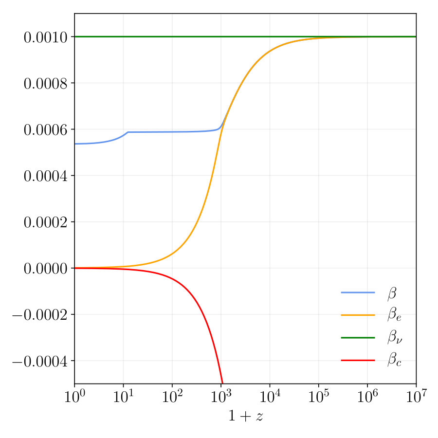 Figure 1
 Figure 2
 Figure 3
 Figure 4
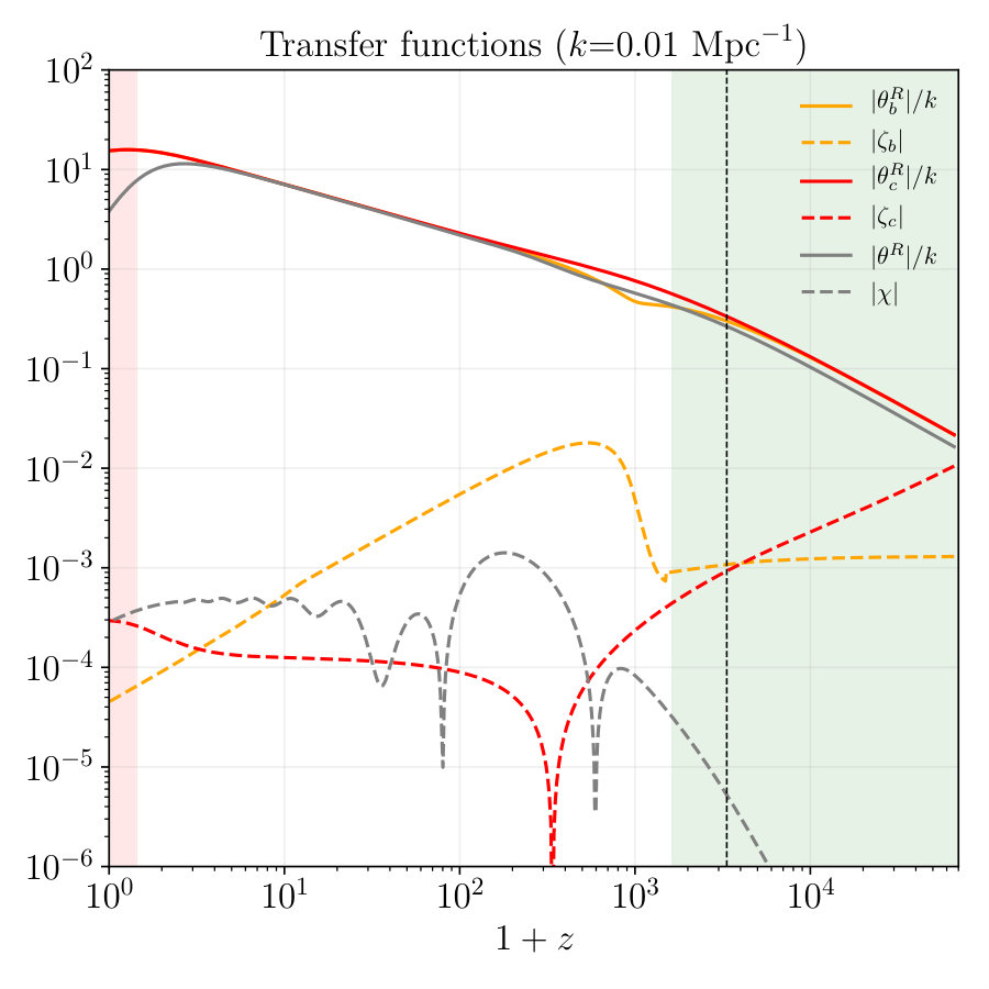 Figure 5
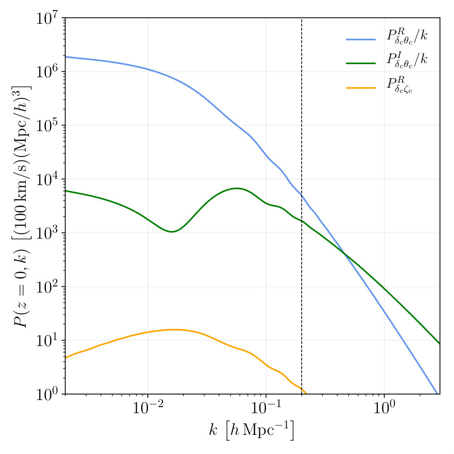 Figure 6
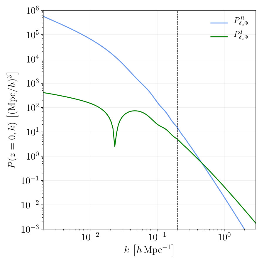 Figure 7
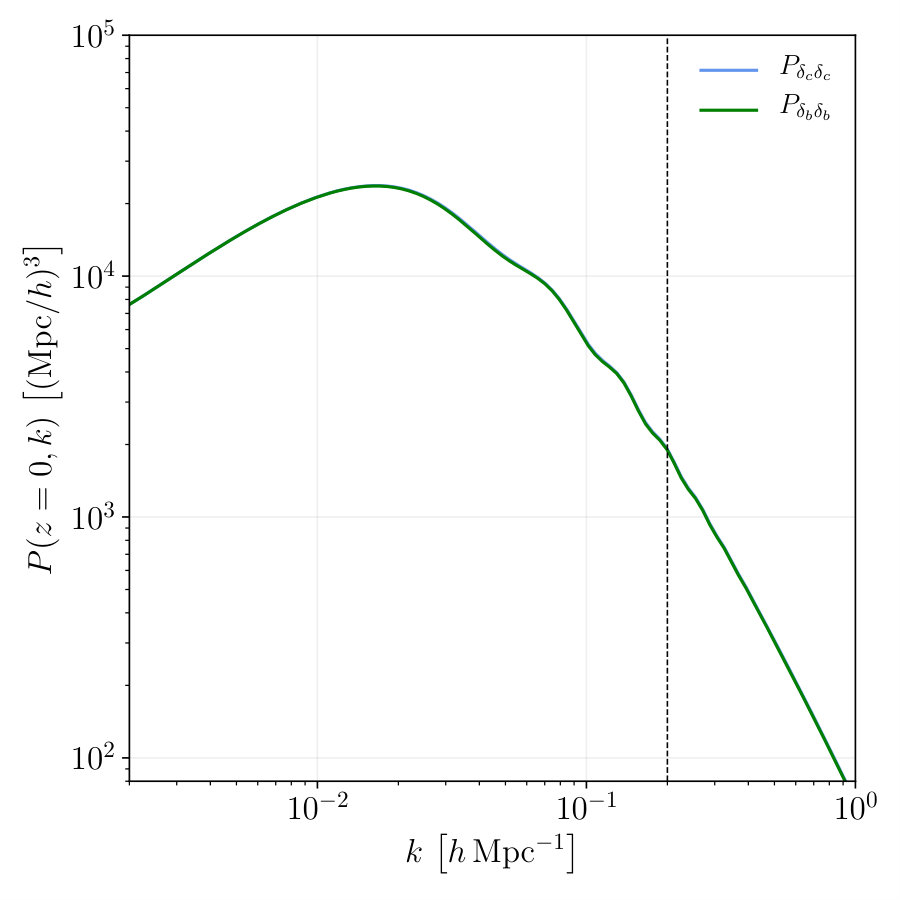 Figure 8
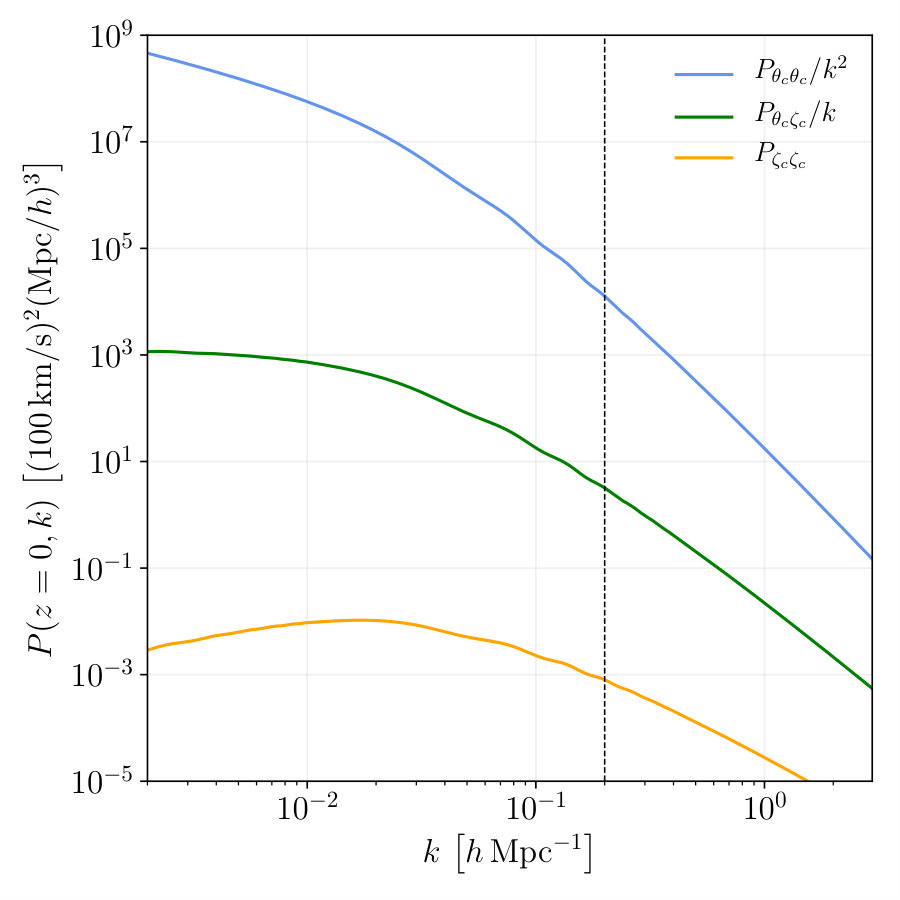 Figure 9
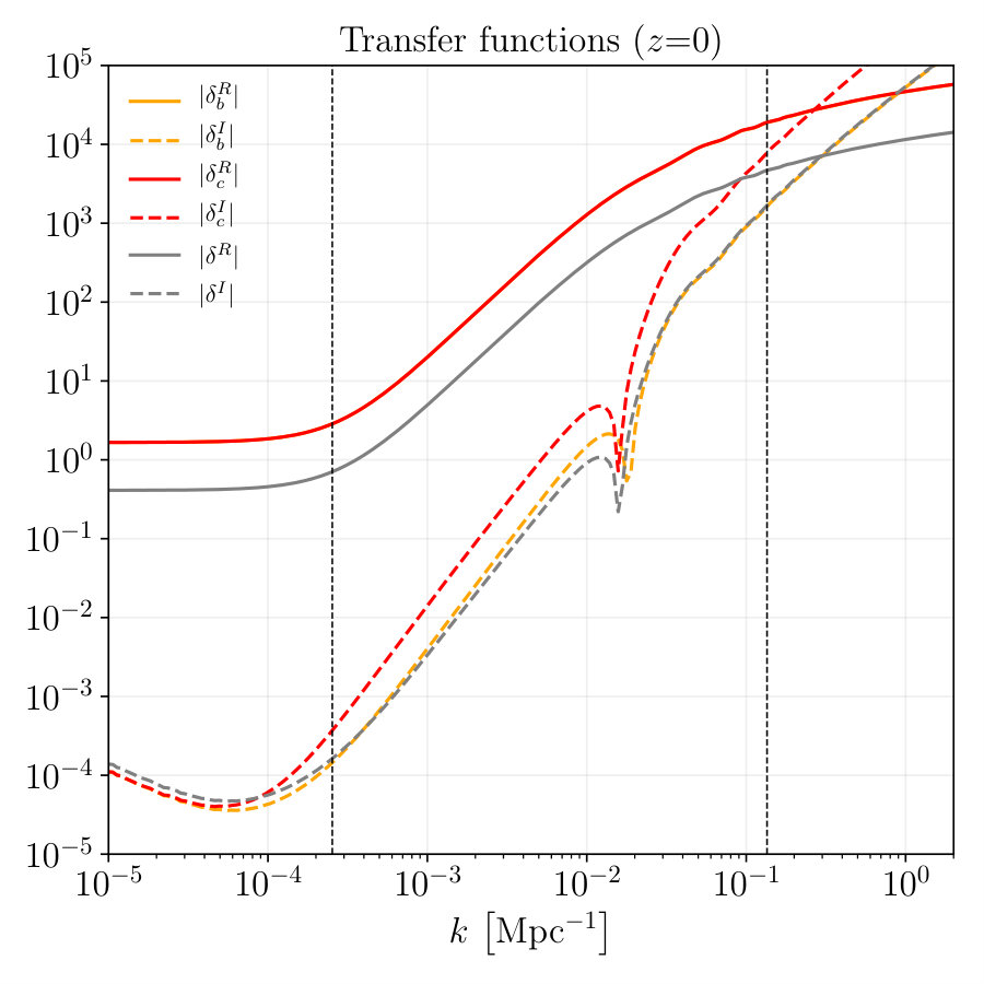 Figure 10
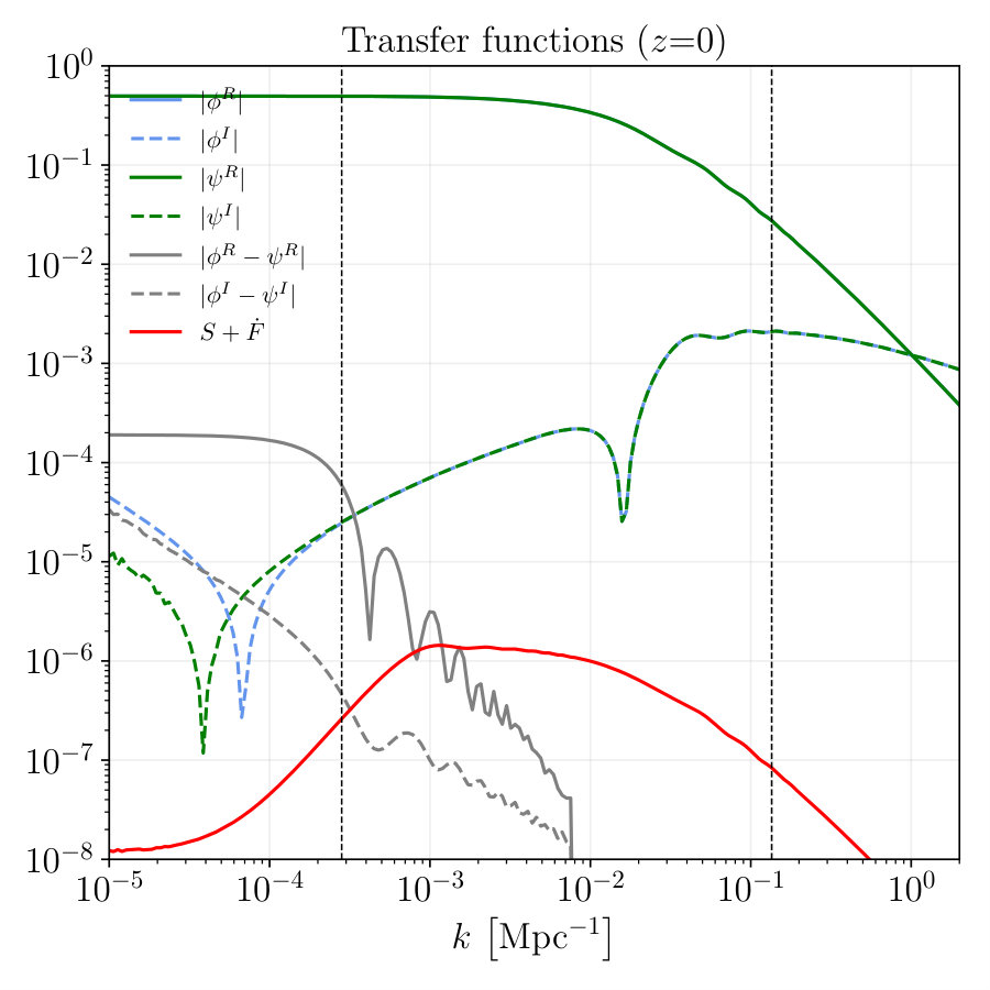 Figure 11
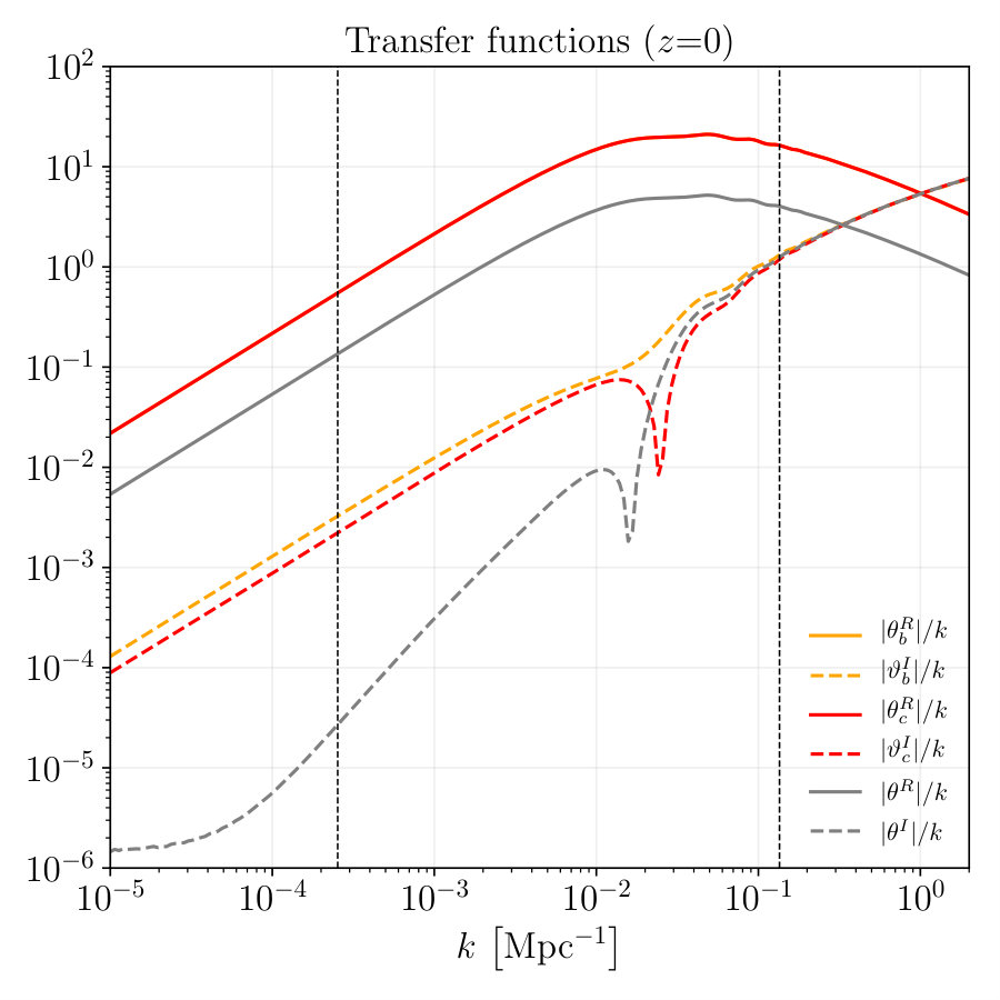 Figure 12
 Figure 13
Peer Reviews
No public reviews on file for this paper yet. If you reviewed it on a platform where reviews are public (OpenReview, ICLR, NeurIPS, ICML), you can paste yours below so the community can read it here.
Videos
No videos yet. Explain this paper in a talk, walkthrough, or lecture? Add one.
Non-comoving Cosmology
J. A. R. [email protected], A. L. [email protected], and H. [email protected]
Departamento de Física Teórica and Instituto de Física de Partículas y del Cosmos IPARCOS, Universidad Complutense de Madrid, E-28040 Madrid, Spain
Abstract
One of the fundamental assumptions of the standard CDM cosmology is that, on large scales, all the matter-energy components of the Universe share a common rest frame. This seems natural for the visible sector, that has been in thermal contact and tightly coupled in the primeval Universe. The dark sector, on the other hand, does not have any non-gravitational interaction known to date and therefore, there is no a priori reason to impose that it is comoving with ordinary matter. In this work we explore the consequences of relaxing this assumption and study the cosmology of non-comoving fluids. We show that it is possible to construct a homogeneous and isotropic cosmology with a collection of fluids moving with non-relativistic velocities. Our model extends CDM with the addition of a single free parameter , the initial velocity of the visible sector with respect to the frame that observes a homogeneous and isotropic universe. This modification gives rise to a rich phenomenology, while being consistent with current observations for (95% CL). This work establishes the general framework to describe a non-comoving cosmology and extracts its first observational consequences for large-scale structure. Among the observable effects, we find sizeable modifications in the density-velocity and density-lensing potential cross-correlation spectra. These corrections give rise to deviations from statistical isotropy with a dipolar structure. The relative motion between the different fluids also couples the vector and scalar modes, the latter acting as sources for metric vector modes and vorticity for all the species.
Contents
I Introduction
The isotropy and homogeneity of the Universe on large scales are two foundational assumptions of the standard cosmological model, the so-called CDM model. These two assumptions are usually grouped under the name of Cosmological Principle. All the observational evidence, ranging from the extremely isotropic cosmic microwave background (CMB) Ade et al. (2016); Akrami et al. (2018) to the galaxy number counts and the measured expansion from SNIa Kolatt and Lahav (2001); Antoniou and Perivolaropoulos (2010); Beltran Jimenez et al. (2015), supports the conclusion that the Universe is very nearly isotropic on large scales. However, the notions of homogeneity and isotropy are inextricably linked with the election of a privileged frame. For any observer moving with respect to this frame, the Universe would appear anisotropic and inhomogeneous. This is precisely our situation on Earth.
Starting with the early CMB measurements Kogut et al. (1993); Lineweaver et al. (1996), a significant dipole modulation, much larger than any other anisotropy, was found. This was readily interpreted as a kinematical effect: a Doppler shifting effect arising from the relative motion of the Earth with respect to the CMB rest frame, i.e. a frame in which the CMB looks isotropic. Recent analysis by the Planck Collaboration Aghanim et al. (2014); Ade et al. (2016) explored other kinematical effects, like the violation of statistical isotropy induced by the observer motion, and reported an independent measurement of our relative velocity with respect to the CMB frame. This measured velocity can, given the uncertainties, fully account for the observed dipole, supporting its kinematical origin. Even if it is mostly kinematical, it may still contain an intrinsic contribution. Some authors have proposed searches for the intrinsic dipole, e.g. using spectral distortions Yasini and Pierpaoli (2017).
A different kind of dipole should appear in the distribution of galaxies, induced by our motion with respect to the matter frame, i.e. a frame in which the matter distribution looks isotropic. The origin of the large scale structure (LSS) dipole lies in a combination of Doppler shifting and aberration effects in the galaxy number counts Ellis and Baldwin (1984); Gibelyou and Huterer (2012). Unfortunately, current observations can only loosely constrain its amplitude and direction, yielding a value compatible with the CMB dipole Condon et al. (1998); Itoh et al. (2010). Future surveys like Euclid Amendola et al. (2018) and SKA Maartens et al. (2015) will measure it with unprecedented accuracy.
To complete the picture, we only need to know the relative velocity between the matter and CMB frames. Concerning this point, CDM contains the underlying assumption, that usually goes by unnoticed, that both frames coincide. CDM assumes matter and CMB to be comoving. As we will see in this work, it is possible to relax this condition. The homogeneous and isotropic Robertson-Walker (RW) metric can be sourced, at the background level, using non-comoving fluids. Thus, we will show that it is possible to construct a viable cosmological model for non-comoving fluids, with interesting phenomenological consequences and without any flagrant isotropy violation.
Early theoretical work concerning non-comoving fluids was mostly developed under the framework of tilted universes. The term was coined in the groundbreaking work by King and Ellis King and Ellis (1973). The authors considered a class of homogeneous models sourced by a single moving fluid, i.e. models in which the fluid 4-velocity is tilted with respect to the homogeneous hypersurfaces. These tilted models produce homogeneous but anisotropic universes. In a different context, Coley and Tupper Coley and Tupper (1986) analyzed two-fluid cosmological models with general imperfect and non-comoving fluids. In order to source homogeneous and isotropic RW metrics, only very special configurations with radial velocities were considered. Later on, Turner Turner (1991) proposed a theoretical mechanism to produce a mismatch between matter and CMB velocities. In Turner’s tilted universes, the presence of a near-horizon-sized perturbation, remnant of inflation, could introduce a spatial gradient, driving the velocity of matter.
The analysis of non-comoving fluids has been extended to dark energy. Given our fundamental ignorance about the behaviour of the dark sector, it is conceivable that it has not ever been coupled to ordinary matter and that it does not share the same rest frame. Following this idea, a model of moving dark energy was proposed in Maroto (2006). In this case, for a dynamical dark energy fluid, even if the matter and CMB frames coincide initially, they differ at late times. Different models of moving homogeneous dark energy were analyzed in Beltran Jimenez and Maroto (2007), as well as its possible impact in observables like the CMB quadrupole. The construction of a fully anisotropic model in which the full dark sector, i.e dark energy and dark matter, is non-comoving with the CMB and ordinary matter was carried out in Harko and Lobo (2013). The authors analyzed a Bianchi I universe in which dark matter and dark energy had different relative velocities with respect to the frame of ordinary matter and then derived some observables, like a modified luminosity-distance relation and CMB quadrupole.
From the observational point of view, a signal of the relative motion of the matter and CMB frames will be the detection of a large-scale bulk flow. In recent years, several works have claimed measurements of matter flows well in excess the CDM predictions on different scales and at different statistical confidence levels Kashlinsky et al. (2009); Ade et al. (2014); Scrimgeour et al. (2016). Although there seems to be a broad agreement on the direction of the flow, the amplitude is still subject to controversy Ade et al. (2014). Such flows will be an indication of the existence of a cosmological preferred spatial direction. On the other hand, detected anomalies in the low multipoles of the CMB temperature power spectrum Ade et al. (2016), such as the low-multipole allignment and the dipolar or hemispherical anomalies, also suggests the presence of a preferred cosmological direction Schwarz et al. (2016). This fact has triggered the search for mechanisms which could break isotropy while keeping the predictions of the standard cosmology.
This work builds upon these previous studies, but we will present the first complete analysis for the evolution of a set of non-comoving fluids, from the early to the late Universe, both at the background and perturbation level. As we will see later, it is reasonable to assume that any pair of tightly coupled fluids share the same velocity. Hence, we can expect that photons, baryons and neutrinos, being in thermal contact in the early Universe, shared a common rest frame, i.e. a frame in which the plasma looked isotropic. However, there is no a priori reason to assume the same about the dark sector. The dark sector, regardless of its composition, may very well possess its own rest frame, with a given global velocity with respect to the visible sector. The only reasonable assumption is that there is one frame that observes a homogeneous and isotropic universe, i.e. a RW background. In this paper we take seriously this possibility and prove, at the background level, that
- •
If the dark and visible sectors are initially moving with non-relativistic velocities, to first order in these velocities, it is possible to define a cosmic center of mass frame that observes a RW background. Our model only contains one additional free parameter , the velocity of the visible sector with respect to the cosmic center of mass frame deep inside the radiation era. As we will see later, is a conservative limit to be in agreement with all observations.
- •
The subsequent evolution gives rise to relative velocities between all the different components of the visible sector, e.g. between baryons and photons, defining each of them its own rest frame.
While at the perturbation level,
- •
There appear couplings, of order , between scalar and vector modes.
- •
There is a production of vorticity for all the species and a net production of vorticity and metric vector modes.
- •
The transfer function of every cosmological quantity acquires a dipolar contribution of order .
- •
There is a violation of statistical isotropy of order . Among the different observables where such an effect could be measured, the easiest to compute is the cross-correlation spectrum between different scalar perturbations, which acquire a dipolar contribution of order .
In this work we will limit ourselves to LSS observables, letting for a forthcoming work the analysis of CMB signatures Cembranos et al. (2019a). The structure of the paper goes as follows. Section II assesses the problem of constructing a homogeneous and isotropic universe using non-comoving fluids. First, only the energy-momentum tensor for a perfect fluid with bulk velocity is considered in II.1, where the conditions for isotropy and homogeneity are discussed. Then, the formalism is extended to imperfect fluids in II.2, using the kinetic approach, where both background and perturbations are studied in II.2.1 and II.2.2. Section III analyzes the dynamics of this model from the point of view of the Boltzmann equations. The free-streaming term is derived in III.1, while the collision term for the photon-baryon plasma is computed in III.2. The main evolution equations are presented in III.3. The usual scalar-vector-tensor decomposition is performed in section IV, where we describe our approximation scheme. Section V contains the Einstein equations, which are not modified in our case. In section VI, we present a reduced version of the original system, under our approximation scheme. Sections VI.1, VI.2 and VI.3 are devoted to bulk velocities, scalar and vector modes, respectively. Finally, section VII contains the numerical solution of the aforementioned reduced system and discusses some observables. Section VIII gathers the main conclusions and presents some prospects for future work.
II Moving fluids
II.1 Perfect fluid with bulk velocity
II.1.1 Physical setting
Let us consider a perfect fluid with energy-momentum tensor
[TABLE]
in a flat Robertson-Walker (RW) metric
[TABLE]
Now we will consider the situation where the fluid possesses a bulk velocity with respect to the frame in which the metric takes the form (2). Parameterizing the four-velocity as
[TABLE]
from the normalization condition, , we have
[TABLE]
where the spatial indices in are lowered and raised using . With this parameterization the components of the energy-momentum tensor are
[TABLE]
Since the non-diagonal components are not zero, this moving fluid cannot act as a source for the geometry (2). Let us show how to construct a valid source for the homogeneous and isotropic metric (2) using a collection of fluids.
Isotropy.
For non-relativistic fluids, the only non-diagonal component, to first order in , is
[TABLE]
If instead of a single fluid we have several fluids in relative motion, they can act as a source for (2) if they satisfy
[TABLE]
The physical content of this condition is that of a kind of center of mass frame condition. An isotropic source can be constructed, to first order in , out of two non-relativistic fluids if the net flux of momentum of one fluid is counterbalanced by that of the other fluid. We will see later that this constraint is conserved in time, so it can be implemented with an appropiate choice of the initial conditions. In Beltran Jimenez and Maroto (2007) it is discussed how to transform to this frame, starting from an arbitrary configuration of the fluids.
Homogeneity.
Homogeneity is easily implemented when the fluids are at rest, but we need to be cautious in our context. Consider two observers locally related by a boost
- •
, frame in which (7) is satisfied and the metric takes the form (2).
- •
, frame moving with respect to with velocity .
In the frame, the transformed coordinates are obtained applying a local Lorentz transformation
[TABLE]
and the metric looks inhomogeneous
[TABLE]
The same applies to other time-dependent quantities like and . To provide a consistent source, we will require that the energy-momentum tensor of each fluid is homogeneous in the frame, i.e. the frame that observes an isotropic and homogeneous metric, not in the comoving frame with the fluid.
Notice that on the tangent space at a given space-time point, we can always define an orthonormal basis given by
[TABLE]
and the corresponding orthonormal basis in the frame reads
[TABLE]
Thus, as expected, the two basis are just related by a Lorentz transformation on the tangent space
[TABLE]
To sum up, we can source a flat RW metric (2) with a collection of non-relativistic moving fluids as long as
- •
We are in the center of mass frame, where
[TABLE]
- •
The energy-momentum tensor is homogeneous in that frame
[TABLE]
II.1.2 Evolution
Finally, in this subsection we will analyze the evolution of a perfect fluid with bulk velocity. Assuming homogeneity
[TABLE]
the conservation equation
[TABLE]
for a flat RW metric in conformal time (2) yields the equations of motion
[TABLE]
where is the conformal Hubble parameter and . As it was anticipated, (18) proves that the center of mass constraint (7) is conserved in time. Writing explicitly the components (5), the equations of motion can be rewritten in terms of and . The equation for the velocity can be expressed as
[TABLE]
where is the equation of state of the fluid. In the absence of interactions, the velocity does not change its direction, so we only need to follow the evolution of its magnitude. Combining (17) and (18), it is possible to obtain
[TABLE]
assuming . It is worth particularizing these results to two kind of fluids.
- •
Radiation, .
[TABLE]
The fluid moves with constant velocity and with the usual scaling .
- •
Matter, .
[TABLE]
The equations can be solved analitically in this case
[TABLE]
where and are the velocity and density today. If the fluid starts with ultrarelativistic initial conditions, it behaves as radiation until the velocity drops down and it enters the non-relativistic regime. In the non-relativistic regime, to first order in , the velocity slows down with the expansion and the density scales as usual .
Analytic expressions for a generic equation of state can be obtained in the regime of small velocities
[TABLE]
where is the value of the equation of state today. For the particular case , we have Maroto (2006); Beltran Jimenez and Maroto (2007)
[TABLE]
II.2 Kinetic approach
Non-relativistic particles and the photon-baryon plasma in the early Universe can be well approximated as perfect fluids, and analyzed using only their energy-momentum tensor. However, to describe the free-streaming of neutrinos or the details of decoupling, the fluid approximation is not enough and we must use a more general kinetic approach. In this section we follow closely the presentation of Ma and Bertschinger (1995).
The phase-space of the system is described by
- •
Three positions .
- •
Three conjugate momenta . These conjugate momenta are defined as the spatial components of the four-momentum
[TABLE]
where is the proper time and the spatial index has been lowered with the full metric .
The number of particles per unit of phase-space volume is
[TABLE]
where is the number of internal degrees of freedom, e.g. the number of helicity states, and is the phase-space distribution function. In the kinetic approach, the energy-momentum tensor can be defined as Ma and Bertschinger (1995)
[TABLE]
where is the determinant of the metric . In a cosmological setting, the next step would be to particularize these definitions to a RW metric (2) and then to study perturbations over the metric and the distribution function. We will split the discussion in two parts. Since our main modification with respect to standard comoving cosmology concerns the definition of the unperturbed distribution function, we will focus on the background in the next section II.2.1. Section II.2.2 contains the complete treatment of perturbations.
II.2.1 Background
Starting again with the metric
[TABLE]
and denoting the momentum as
[TABLE]
such that , we obtain from the mass-shell condition (33)
[TABLE]
We introduce again two related frames.
- •
, frame in which the metric takes the form (36).
- •
, frame moving with respect to with velocity .
The local Lorentz transformation (8) that connects both frames yields
[TABLE]
We have defined
[TABLE]
where is a unit vector along and every spatial index has been lowered or raised with . Next we consider a homogeneous distribution function in the frame
[TABLE]
With this distribution function, we can define the usual fluid quantities
[TABLE]
that represent the usual energy, momentum, shear tensor, pressure, number and velocity densities of the fluid. To relate this set of quantities with those computed in the boosted frame, we can either use their tensorial character under local Lorentz transformations or the fact that transforms as a scalar
[TABLE]
where, from now on, we will denote \tilde{f}_{0}(\tilde{\tau},\boldsymbol{\tilde{x}},\boldsymbol{\tilde{q}}\big{)} just as . With this property and the Lorentz-invariant volume element we can write, for instance,
[TABLE]
Using this procedure, one can obtain
[TABLE]
It is important to stress that the preceeding relations hold as well if the quantities are defined with the full distribution function , instead of using just the background part , and we will make use of them when we study perturbations.
There remains the question of how to describe the moving fluids of section II.1 in terms of a distribution function. We will describe the different constituents of the universe with an unperturbed distribution function that satisfies
[TABLE]
That is, the distribution function is homogeneous in the frame, i.e. the frame that observes a homogeneous and isotropic universe, and isotropic in the frame, i.e. the frame comoving with the fluid. This parallels the discussion in section II.1 and allows us to describe a fluid moving with velocity . The condition (46) is the main physical assumption in our work. For instance, applying it to a black-body spectrum for massless particles, using (39) we obtain the usual boosted distribution function
[TABLE]
If the distribution function satisfies (46) we have
[TABLE]
so we are indeed in the comoving frame with the (perfect) fluid. In this case, the relation between both sets of fluid variables is
[TABLE]
Using the definition of the energy-momentum tensor (35), we can write its components as
[TABLE]
These expressions agree with the ones obtained for a perfect fluid (5). Both approaches are equivalent at this level. To first order in we have
[TABLE]
The full energy-momentum for a collection of fluids is homogeneous, as it was imposed in (46), and it is also isotropic, to first order in , if the velocities of the fluids satisfy the constraint
[TABLE]
which is the same condition obtained in (7). It is clear from (50b) that a similar constraint can always be imposed, to all orders in , to achieve but this is not enough to source a RW geometry. Already to second order in , (50c) contains a quadrupolar anisotropy that cannot be compensated by the other fluids. In this case, we should go one step further and consider a Bianchi universe. However, for the values of that we will consider, this quadrupole lies well below the observed value Beltran Jimenez and Maroto (2007). Therefore, in this work we will restrict ourselves to first order and a RW background.
II.2.2 Perturbations
Our starting point now is a perturbed flat RW metric
[TABLE]
Reparameterizing the momentum as
[TABLE]
from the mass-shell condition (33) we obtain
[TABLE]
These expressions can be regarded just as redefinitions but they have a very simple physical interpretation in terms of the vierbein (11). Our choice of momentum, , corresponds to a choice of vierbein with components
[TABLE]
With these definitions, are the momenta measured by a locally inertial observer at a fixed spatial position. It is convenient to work with a closely related set of variables defined as
[TABLE]
As we will see, written in terms of , the Boltzmann equation in section III does not contain a zero-order term. We perturb the phase-space distribution accordingly
[TABLE]
and define the corresponding perturbed fluid variables
[TABLE]
The components of the perturbed energy-momentum tensor are
[TABLE]
Expressing the background quantities in the frame
[TABLE]
It is easy to show that, to first order in , once we apply the center of mass condition (52), every metric variable cancels out and does not appear in the definition of the total energy-momentum tensor.
Non-relativistic limit
We end this section with an aside about the non-relativistic (NR) limit (). In the next sections only massless (photons and massless neutrinos) and NR particles (baryons and cold dark matter) will be taken into account. In particular, we will only keep the first NR order, neglecting the pressure and sound speed of baryons.
Although this kind of approximation is standard, we must be careful when taking the NR limit in a moving frame. The proper way to account for this limit is to take it in the frame comoving with the fluid, i.e. . To first NR order we have
[TABLE]
However, in the frame, using (45), it can be seen that we do have pressure and anisotropic stress
[TABLE]
To first NR order and to first order in , we have the following useful results
[TABLE]
Note that the preceeding results hold as well for the corresponding unperturbed quantities, see (II.2.1). Finally, the full energy-momentum tensor for a non-relativistic species to first order in is
[TABLE]
III Boltzmann equation
After writing the energy-momentum tensor in terms of the distribution function, we need to compute its time evolution. This information is encoded in the Boltzmann equation, which in the locally Minkowskian frame takes the form
[TABLE]
where is the time measured by the locally Minkowskian observer, which for the vierbein choice in (56) reads . The left-hand side, the so-called Liouville operator, describes the free streaming of particles in phase space. It is defined as
[TABLE]
This operator contains the information about the space-time geometry, through its effects on the geodesics of the particles. The functional on the right-hand side of (66) is the so-called collision term. It takes into account how the number of particles per unit of phase-space volume change due to collisions, i.e. local interactions. Hence, it does not contain information about the underlying geometry Bernstein (1988). The collision term takes the same form as in flat space-time when written in terms of the momenta measured by a locally inertial observer defined above. The final form of the Boltzmann equation in conformal time is
[TABLE]
The next section is devoted to the left-hand side of the Boltzmann equation, i.e. the Liouville operator, particularizing to massless and non-relativistic particles. This analysis exhausts all the information needed to follow the evolution of non-interacting particles, like CDM and neutrinos. However, to describe the photon-baryon plasma, we must move on to the full Boltzmann equation. Section III.2 studies the interaction between photons and electrons.
III.1 Liouville operator
In order to compute the time derivatives appearing in (67), we need the geodesics in the metric (53). The whole computation of the geodesics can be found in detail in the appendix A. Using the definition of the four-momentum (33) and the parameterization (54), the final results are
[TABLE]
where the following combinations of metric variables have been defined
[TABLE]
The left-hand side of the Boltzmann equation (68) is evaluated in the frame, where the geodesics are computed,
[TABLE]
We will assume that the distribution function takes the form
[TABLE]
where is the standard isotropic distribution in the frame. Since (69b) is already first order in perturbations, the left-hand side of the Boltzmann equation can be recast as
[TABLE]
We will restrict our discussion to massless and non-relativistic massive particles.
III.1.1 Massless particles
For massless particles the Lorentz transformations (39) take a simpler form
[TABLE]
where we have splitted the momentum into direction and magnitude
[TABLE]
Using the Boltzmann equation, it can be directly checked that the unperturbed distribution function in the frame only depends on , if there is no zero-order collision term,
[TABLE]
It is convenient to work with the reduced phase-space density, integrating out the dependence on the momentum magnitude, defined as
[TABLE]
where the constant is related to the comoving energy density
[TABLE]
Plugging the geodesic equation (69) into the right-hand side of (73) and integrating over the momentum magnitude, we obtain, to all orders in ,
[TABLE]
Expanding it to first order in , we have
[TABLE]
The first moments of the angular distribution can be obtained performing the appropiate integrals
[TABLE]
where we have defined
[TABLE]
III.1.2 Massive particles
The results for massive particles are much more involved. In this case, we must use the full expressions for the Lorentz transformations (39) and the geodesics (69). However, since we will focus on non-relativistic particles, we can simplify the analysis restricting it to the first moments of the Boltzmann equation. Summing up, in this section we compute the evolution of the number density, energy and velocity perturbations.
The energy density contrast, equation of state and sound speed are defined as
[TABLE]
Note that in these definitions the background quantities are referred to the frame while the perturbed quantities are defined in the frame. The election of intermediate variables is a matter of choice, the only condition being that we write the energy-momentum tensor consistently in terms of these variables. We stick to this convention throughout this work. The final results for the first moments of the distribution are
- •
Number density.
[TABLE]
- •
Energy.
[TABLE]
- •
Momentum.
[TABLE]
These results are exact to all orders in , for relativistic and non-relativistic particles alike. They can be shown to reproduce (81) and (82) for massless particles. Next we define
[TABLE]
Assuming that the zero-order Boltzmann equation (without collisions) is satisfied, so we keep only cosmological perturbations and terms with , and expanding to first NR order and to first order in we have
- •
Number density.
[TABLE]
- •
Energy.
[TABLE]
- •
Momentum.
[TABLE]
III.2 Collision term
This section is devoted to the calculation of the collision term for Compton scattering between electrons and photons. The notation in this section is slightly different. As we mentioned before, the collision term must be written in terms of the momenta measured by a locally inertial observer at a fixed spatial position. They are related to the momenta we have been using as defined in (57), i.e. .
The standard physical assumptions underlying the derivation of the collision term are
- •
When written in terms of the momenta , the collision term is the same as in flat space, since it takes into account local information where the curvature effects are not important. In the same way, the matrix element is computed using quantum field theory (QFT) in flat space.
- •
The temperature of the plasma is low enough so that the electrons are non-relativistic. We keep only the first order correction in the non-relativistic expansion, so we keep the electron velocity but neglect its pressure and sound speed. We consider the NR limit of Compton scattering, i.e. Thomson scattering.
- •
Electrons and protons are much more tightly coupled between them than to the photons. The velocities of free electrons, protons and the full baryonic velocity are the same throughout the evolution.
- •
The angular dependence of Thomson scattering is neglected. This angular dependence has proven important for 1% accuracy and especially for polarization, but we will not take it into account in this work. We use the angle-averaged matrix element instead.
- •
The number of internal degrees of freedom is not included in the definition of , i.e. the equilibrium distributions correspond to the usual Bose-Einstein and Fermi-Dirac distributions.
- •
The medium is diluted enough so that we can neglect the quantum statistical factors responsible for the Bose enhancement and Pauli blocking effects. We do not take into account any plasma effect from finite temperature QFT.
With these qualifications, our starting point is the following definition of the collision term for the process
[TABLE]
where is the Lorentz-invariant phase-space volume element and the dependence of the distribution functions on space-time coordinates has been omitted since it does not play any role. In our setting, we must implement the fact that the fluids are moving. The collision term is defined in the cosmic center of mass, frame, and in this frame both photons and electrons have their own bulk velocity. We will represent it schematically as
[TABLE]
where and are the distribution functions of photons and electrons in their frame, moving with bulk velocities and , respectively, with respect to the frame.
Previously, the frame was defined as the frame comoving with the fluid. In this case, we are facing two moving fluids. We take to be the frame moving with velocity with respect to , i.e. the frame comoving with the electrons. Performing the integration in this frame, we have
[TABLE]
The previous two equations may seem devoid of any additional content with respect to (92). As they stand, without defining and , they correspond just to a renaming of functions and reshuffling of variables. The physical content lies in (III.1), i.e. in the structure and relation of the background distribution function in and . The frame is comoving with the electrons and observes a standard isotropic equilibrium distribution. It is in this frame that we can perform the usual NR expansion Dodelson (2003) to get
[TABLE]
where is the Thomson cross section and we have defined
[TABLE]
where , correspond to the full distribution functions. Just as we did for the left-hand side in section III.1, we will split the distribution functions into a background and a perturbation part and integrate out the magnitude of the photon momentum. The whole process, to all orders in , is detailed in the appendix B. Here we present only the final results. To first order in , we get
[TABLE]
where is the number density of free electrons in the frame, and are defined in (88) and the difference of velocities is
[TABLE]
Since, to first order in , the background quantities like or concide in the and frames, we will drop the distinction. The first two moments of the photon collision term are
[TABLE]
Conserved quantities
We have just computed the collision term for photons. However, the whole plasma is described by the coupled system
[TABLE]
We ought to compute the collision term for electrons as well. Not surprisingly, both terms are not independent. In fact, we can make use of some conservation laws derived from the full Boltzmann equation to save us most of the work. Following Dodelson (2003), we write both collision terms with the compact notation
[TABLE]
Integrating over all the momenta, it is easy to see that we have
[TABLE]
corresponding to the conservation of the number of particles, energy and momentum. Using these results, the following equalities hold
[TABLE]
This means that we can compute the first two moments of the Boltzmann equation for electrons, the only ones that we will need since they are non-relativistic, from the first two moments of the photons, already computed in (99) and (100).
III.3 Boltzmann equation for different components
III.3.1 Photons
The reduced Boltzmann equation for photons is obtained combining the Liouville operator (III.1.1) and the collision term (III.2). To zero order in cosmological perturbations, it describes the evolution of the bulk velocity
[TABLE]
To first order in cosmological perturbations and , we get the evolution of the reduced phase-space density
[TABLE]
Since protons and electrons form a single tightly coupled baryonic fluid, we have substituted with , the velocity of baryons. The evolution of the fluid variables can be obtained performing the appropiate angular integrals. The equations for the density, combining (81) and (99), and the velocity, combining (82) and (100), are
[TABLE]
III.3.2 Baryons
The evolution of the baryon density can be found using the left-hand side (90) and energy conservation (106). For the velocity, we must use the left-hand side (• ‣ III.1.2) and momentum conservation (107). As mentioned before, since they are much more tightly coupled between them than to photons, electrons and protons form a single baryonic fluid. We use to denote the baryon velocity. To zero order in cosmological perturbations, we find the evolution of the bulk velocity
[TABLE]
To first order in cosmological perturbations and , the evolution of the first two moments of the distribution is
[TABLE]
III.3.3 Massless neutrinos
Since we will neglect both the mass and coupling of neutrinos, they only free-stream with the same left-hand side as photons. The equation for is
[TABLE]
The equation for the evolution of the reduced phase-space density is
[TABLE]
III.3.4 Cold dark matter
Cold dark matter behaves as collisionless non-relativistic matter, i.e. it just follows the same equations as baryons without interactions. The equation for is
[TABLE]
The relevant equations for the perturbations are
[TABLE]
III.3.5 Total fluid
The total energy-momentum tensor, adding all the components, does not contain any explicit contribution after enforcing the cosmic center of mass condition. The conservation of the total energy-momentum tensor, which is a direct consequence of the Einstein equations,
[TABLE]
gives us the conservation and Euler equations for the total fluid
[TABLE]
where the different variables are defined in the same way as for the individual components, but using the total energy-momentum tensor, e.g.
[TABLE]
IV Multipole analysis
The cosmological perturbations can be classified according to their transformation rules under the group of spatial rotations. This yields the usual splitting in scalar, vector and tensor perturbations, the only ones that contribute to the Einstein equations. Additionally, in the standard cosmological perturbation theory, the three types of perturbations are decoupled at the linear level, a fact known as decomposition theorem Kodama and Sasaki (1984). Since, in this case, the only angular contribution comes from factors of the form , i.e. the angle between the line of sight and the direction of the Fourier mode, it is customary to write a multipole expansion for the scalar part of the Boltzmann equation (III.3.1) in terms of Legendre polynomials Ma and Bertschinger (1995)
[TABLE]
The Boltzmann equation then unfolds into a whole hierarchy of coupled differential equations for the coefficients . The vector modes are usually neglected altogether since, even if initially present, they rapidly decay. The tensor modes are predicted in small quantities in many inflationary scenarios and their evolution must be followed when studying polarization effects.
The key difference in our scenario is the existence of a new direction , introducing new angular dependencies in the Boltzmann equation (III.3.1). This means that we must resort to a full decomposition in terms of spherical harmonics of the form
[TABLE]
where the coefficients have been defined to match the previous ones for the scalar modes. In particular, in our case, the decomposition theorem no longer holds. As it can be checked, in addition to the usual coupling between and modes, the term introduces new couplings between the modes and . It is possible to write down the new hierarchy of coupled differential equations for the modified Boltzmann equation (III.3.1) and it is important for a correct computation of CMB anisotropies Cembranos et al. (2019a). However, in this work we are mainly concerned with LSS observables and we do not need to trace the evolution of ultrarelativistic species with high accuracy. Therefore, we will be working under an approximation scheme that allows us to consider only a subset of these equations. Consequently, we present in this section a self-contained simplified derivation of the system of equations that we will solve in later sections, bypassing the full multipole decomposition.
IV.1 Scalar-vector-tensor decomposition
Any spatial vector, in particular the velocity, can be decomposed into a divergence and a divergenceless part
[TABLE]
where is the scalar part of the velocity and is the vector part, the vorticity. In Fourier space, it can be written as
[TABLE]
A spatial traceless tensor can be decomposed in a similar way
[TABLE]
where again the vector part is divergenceless and is the tensor part, satisfying
[TABLE]
Alternatively, we can write it in Fourier space as
[TABLE]
according to the notation of Ma and Bertschinger (1995) for the scalar part of the shear tensor, . Adapting the notation of Mukhanov et al. (1992) for a generic gauge, the metric perturbations can be decomposed as
[TABLE]
where and are vector perturbations, i.e. divergenceless vectors, and is a tensor perturbation, i.e. a divergenceless and traceless tensor. Our previously defined variables for a general metric perturbation (53) now take the form
[TABLE]
From now on it will be convenient to work in Fourier space and to choose a basis adapted to the previous decomposition. The components of the line-of-sight vector are
[TABLE]
where we have chosen the so-called helicity basis Durrer (2008)
[TABLE]
and our convention for the spherical harmonics matches those of Durrer (2008) or Arfken and Weber (1999).
IV.2 Lower moments evolution
The first moments of the Boltzmann equation have already been obtained in the previous sections, with corresponding to the density (110) and to the velocity (111). The next moment can be obtained via direct integration of the Boltzmann equation (III.3.1) and corresponds to the shear tensor (83c). Performing the appropiate integral, we have
[TABLE]
To obtain the scalar, vector and tensor parts of this expression, we compute the components as
[TABLE]
The projection of a vector in the helicity basis is computed in a similar way
[TABLE]
Projecting the equations of motion we obtain
[TABLE]
where it is easy to check that the projections correspond to the scalar part and one of the two vector and tensor helicities
[TABLE]
There remains to perform a couple of angular integrals, writing down the appropiate coefficients of the expansion (126) and to substitute the metric variables defined in the previous section (IV.1). After these simplifications, and rearranging terms, the first moments of the Boltzmann equation for photons are
Scalar.
[TABLE]
Vector.
[TABLE]
Tensor.
[TABLE]
The corresponding results for the other helicity can be obtained substituting in every sub and superscript.
Several comments are in order now. In the first place, note that all the couplings between scalar, vector and tensor modes are introduced by terms proportional to . In the standard case, each mode evolves independently. In the second place, note the appearance of terms with . What we present here are but the lowest moments of a whole hierarchy of coupled differential equations. This system obeys a recurrence relation but it must be truncated at a finite, prefearably large, value of . The traditional line-of-sight approach Seljak and Zaldarriaga (1996) was developed to allow a truncation at lower , and it is used by every modern Boltzmann solver Lewis and Bridle (2002); Blas et al. (2011). It will not be used here, even though it can be adapted to our case Cembranos et al. (2019a), since we are mainly interested in the matter power spectra and not in the CMB. Instead, we will study a simplified version of the system, under the following approximations.
- •
We will work to first order in and to first order in cosmological perturbations, keeping cross-products. We have been implicitly working under this assumption, since the RW background is only correct to first order in , but we will consistently carry it through.
- •
We will assume that there are no initial vector or tensor modes to zero order in . The assumption is justified for vector modes, since most popular models of inflation do not produce them at all. On the other hand, since we have not detected tensor modes so far, and we have stringent limits on their amplitude, we assume that their amplitude is small enough so we can neglect them.
Under this assumption, the hierarchy is simplified. Since they are zero initially the only production occurs through their new couplings, i.e. it is proportional to . The vector modes are then and the tensor modes are . In general, we can neglect the backreaction of higher modes into lower modes. As we will see in the next section, the Einstein equations are not modified, so we can apply the same reasoning to the metric variables, i.e. and are and is .
- •
The last approximation is the so-called fluid approximation. We will truncate the hierarchy at for scalar and vector modes. This is a classic working assumption in approximate computations of the CMB, that may introduce up to 10% errors in computations of the CMB spectrum Hu et al. (1995). Another source of error in our case is the naive truncation scheme we are using, i.e. setting to zero all higher moments. It is a well known fact that this truncation scheme, neglecting the damping produced by the transfer of power to higher moments, produces some spurious growth at small scales in the ultrarelativistic species. Since, in this work, we are not interested in following with great precision the evolution of photons or neutrinos, and we have checked that they have a negligible impact in our final results, we will nonetheless stick to this crude truncation scheme in our numerical solutions.
To increase the accuracy of the results for ultrarelativistic species one would need to evolve the full hierarchy Cembranos et al. (2019a), or at least introduce a better truncation scheme Ma and Bertschinger (1995) or an effective viscosity in the equations of motion for ultrarelativistic species Hu (1998).
V Einstein equations
In this section we present the last piece of information needed to solve the system: the evolution of the metric perturbations. It is worth remembering that, to first order in , the background quantities we are interested in, e.g. and , are equal in the and frames. Hence, as in previous sections, we will drop the distinction. The full energy-momentum tensor for each component is
[TABLE]
where is different for each component. We must write now the Einstein equations with this source for the metric (IV.1). For the background evolution we obtain the standard Friedmann equations plus a condition for the cosmic center of mass frame
[TABLE]
Applying the condition (151), the explicit contributions to the full energy-momentum tensor vanish
[TABLE]
In our case the non-relativistic species have pressure and anisotropic stress of order . Splitting the sources into relativistic and non-relativistic components we have
[TABLE]
Finally, the Einstein equations read
- •
[TABLE]
- •
[TABLE]
- •
[TABLE]
Again, the results for the helicity can be obtained substituting in every sub and superscript. With our notation, the Newtonian gauge can be obtained just setting and the synchronous gauge is defined as
[TABLE]
The Einstein equations in the synchronous gauge for scalar perturbations can be written as
[TABLE]
where we have defined
[TABLE]
Appendix C contains a discussion about how the gauge transformations are modified for non-comoving fluids and, in particular, how to relate the Newtonian and synchronous gauges.
VI Reduced system and final equations
This section contains the final, simplified equations that will be numerically integrated. In the first place, the relevant equations for the evolution of the bulk velocities are presented in section VI.1. The background follows the standard CDM evolution to first order in , but there is a first order effect on the perturbations.
Once the evolution of the bulk velocities is known, we need to study the modified evolution of the perturbations. Working to first order in and with the approximations made at the end of section IV, our modifications to the scalar and vector modes decouple and can be treated separately. This is the subject of the last two sections VI.2 and VI.3. As mentioned before, the tensor modes are second order in and we neglect them.
VI.1 Bulk velocities
The evolution of the velocities of the different fluids is governed by
[TABLE]
where we have defined
[TABLE]
and, as we mentioned before, the initial conditions are chosen according to the constraint
[TABLE]
so the cosmic center of mass condition is maintained in the evolution. Moreover, we will assume that all the bulk velocities are aligned along the axis in the frame. As we will shortly see, and can be inferred from (171a) and (171c), when two species are tightly coupled their velocities evolve to become equal. Once a particle species decouples, the magnitude of its velocity evolves independently but, in the absence of additional interactions or other sources of anisotropy, it does not change its direction. In our scenario, we assume that the whole visible sector has been in thermal equilibrium at some time so all its components, even if they are decoupled like the neutrinos, have velocities pointing in the direction . The only remaining contribution is the dark sector, with DM among its components. The dark sector in the frame counterbalance the flux of momentum of the visible sector to achieve an isotropic universe, so it must point in the direction.
CDM and neutrinos are decoupled, but the photon-baryon system must be treated with some care. In the tight coupling limit, , it is easy to see that the velocities converge in direction and magnitude and we can look for an approximate solution of this system. Expanding perturbatively in the small parameter we have
[TABLE]
The differential equation can be solved to yield
[TABLE]
where is the initial velocity of the visible sector in the frame, the only additional free parameter in our model. In a similar way, the neutrino and CDM equations can be solved to give
[TABLE]
Using the scaling (178) and enforcing the constraint (173) during the tightly coupled regime, the value of is found to be
[TABLE]
It is important to notice that according to the evolution of (178), early enough in time, the condition could break down. However, this is only the case if the DM keeps the non-relativistic distribution at early times. If the DM were light enough it could behave as a radiation-like fluid well before its bulk velocity reaches . In this case, would remain constant and small. On the other hand, if the DM is heavy, its bulk velocity can reach the relativistic regime. In this case, it is worth mentioning that even if the anisotropies that would arise at the background level are and not , their effects can only be relevant well before the matter-dominated era, with no observational consequences.
In order to avoid choosing any particular framework for the dark sector, we will not follow the dark matter evolution using (178). Instead, we follow the evolution of photons (171a), neutrinos (171b) and baryons (171c), and then the momentum of the dark sector, regardless of its composition, can be obtained imposing the center of mass condition (151). Thus, our only assumptions regarding the dark sector are that it is subdominant at early times and that it behaves as cold matter plus cosmological constant at late times.
VI.2 Scalar modes
Here we provide the scalar mode equations for the photon-baryon system. Neutrinos and CDM obey the same equations as photons and baryons, respectively, without the coupling term, i.e. . In addition to the definitions (VI.1) we define
[TABLE]
The evolution of the photon perturbations is described by the equations (143, 144, 145). Under the approximation scheme discussed at the end of section IV, i.e. neglecting backreaction of vector modes and neglecting moments higher than , these equations take the form
[TABLE]
Neutrinos are described by the same system, without collision term. For baryons, we apply our approximation scheme to equations (113) and (114) obtaining
[TABLE]
Again, CDM equations take the same form, but without collision term. The evolution of the full energy-momentum tensor is described by
[TABLE]
where
[TABLE]
The system of cosmological perturbations is a system of linear differential equations. A generic cosmological perturbation can be written as a product of a primordial perturbation, encoding the initial condition, and a transfer function, encoding the subsequent evolution Liddle and Lyth (2000)
[TABLE]
As long as we consider only the adiabatic mode, every cosmological perturbation is proportional to the primordial curvature perturbation . Furthermore, since the system is linear, it can be recast into a system for the evolution of the transfer functions with the substitution . It is common practice to abuse slightly of the notation and to denote as , the perturbation itself, and to solve the system as if it had initial conditions . The information about the initial conditions is recovered later, in the computation of the physical spectra, convolving the transfer function with the primordial spectrum. We follow this practice.
An important difference in (181) and (182) with respect to the case is the appearance of imaginary terms. Usually, even though the Fourier coefficients are generally complex, the evolution equations are real. In this case, both real and imaginary part of satisfy the same equation and with a judicious choice of initial global phase it can be made purely real. With the appearance of complex coefficients, real and imaginary parts form a coupled system with different equations of motion.
We will assume that the global phase has been chosen so that the imaginary parts are initially zero, or at most . Even if they are initially zero, the terms proportional to couple the imaginary to the real parts, driving them to a finite value proportional to . Then we are in the same situation as with the vector modes. The imaginary parts of the scalar modes are determined by the real parts, but they do not backreact on them. The real parts follow the standard cosmological evolution. Therefore, every perturbation transfer function can be splitted as
[TABLE]
where now and are purely real and do not depend on the direction of . Following this definition and the previous discussion, we are in the following situation.
- •
The real part of the perturbations only contains adiabatic perturbations, as in standard CDM, and follows the standard evolution.
- •
The real parts act as external sources in the system for the imaginary parts, via contributions . The imaginary parts of the perturbations are .
We will work in the synchronous gauge (165). The modified gauge-transformation properties are provided in the appendix C. Written in the synchronous gauge, the final system for the photon perturbations is
[TABLE]
The equations for neutrinos are the same, setting the collision part to zero. For the baryons we have
[TABLE]
And finally for the full fluid
[TABLE]
where, in the synchronous gauge,
[TABLE]
To complete the system, we compute the variables and using a combination of the Einstein equations
[TABLE]
Usually, one would integrate the equations for photons, baryons, neutrinos and CDM. Then, after adding all the components, one would compute the sources for the metric perturbations, i.e. the full energy-momentum tensor. As we mentioned before, in our setup we have found it more convenient to follow a different route. Instead of tracking the behaviour of the dark sector, thus choosing a particular DM framework, we follow the evolution of the whole fluid (190). Using these equations, the only underlying assumptions are
- •
The dark sector is subdominant with respect to neutrinos and photons at early times, i.e. before the matter-domination era.
- •
There is a transition to a CDM behaviour at late times.
Under these assumptions, the only CDM contribution to the full fluid goes into the equation of state , since in the synchronous gauge it does not contribute to or at first order in . The evolution of the dark sector can be obtained afterwards subtracting the contributions of photons, baryons and neutrinos from the full fluid.
We are in position now to numerically solve the system. Our strategy can be summarized as follows.
- I)
The background and the real part of the perturbation, labelled with , follow the standard evolution and act as external sources in our system. We use class Blas et al. (2011) to precompute these sources and then solve numerically the system for the imaginary parts, labelled with . The equations for the evolution of are (171a), (171b) and (171c). 2. II)
The system to be solved for the imaginary parts consists of (188), (189), (190), (193), (194) and a neutrino contribution equal to (188) but without collisions. 3. III)
The initial conditions are discussed in the appendix D, where we find the analytic super-Hubble behaviour of the perturbations. In addition to the usual adiabatic and isocurvature modes Bucher et al. (2000), we find a “sourced mode” that depends on the initial value of , i.e. the standard initial curvature perturbation in the adiabatic mode. If we assume that , since they have been thermally coupled at some point, the presence of these external sources introduces an isocurvature velocity perturbation
[TABLE]
where is the initial value of the velocity of photons and neutrinos. All other perturbations are assumed to be initially zero. The whole analysis and the series expansions are described in the appendix D. 4. IV)
The impact of perturbed recombination Naoz and Barkana (2005); Lewis (2007) is usually neglected but it will be important in our case. This subject is covered in section VI.2.1. 5. V)
We need two approximation schemes to follow the numerical evolution, the so-called tight coupling approximation (TCA) and radiation streaming approximation (RSA). We use the same criteria and switches as class Blas et al. (2011). The appropiate equations for TCA are presented in section VI.2.2. While TCA is important at early times, RSA is crucial at late times, when the ultrarelativistic species are decoupled and start oscillating fast. In this case, it is time consuming to follow every oscillation but it is not necessary since at late times the impact of ultrarelativistic components on the metric potentials is negligible. We describe this scheme in section VI.2.3.
VI.2.1 Perturbed recombination
The disturbances in the photon temperature field produce perturbations in the ionization fraction of the electrons. In standard CDM, this inhomogeneous recombination produces second order effects in the CMB, but it has proven important at late times when computing other observables like the 21 cm radiation, through its effects in the gas temperature Naoz and Barkana (2005); Lewis (2007).
Boltzmann codes like camb Lewis and Bridle (2002) and class Blas et al. (2011) have implemented perturbed recombination at late times. This implementations follow the formulae of recfast Seager et al. (2000), including perturbations into the recombination coefficient that effectively takes into account multilevel atom computations. These codes also track the evolution of the gas temperature and its perturbations, that modify significantly the baryon sound speed.
The study of the dark ages in detail is beyond the scope of this work, but, in our case, perturbed recombination plays a role in the photon-baryon system to first order in , where a perturbation in the number of free electrons appears, e.g. see (III.3.1). The baryon sound speed has been neglected in our calculations, it is only important at very small scales, and we will neglect the perturbations in the gas temperature and the recombination coefficient as well. Defining the ionization fraction Kolb and Turner (1990); Seager et al. (2000) as
[TABLE]
where and are the number densities of free electrons and baryons, respectively, we have
[TABLE]
where is the relative perturbation in the ionization fraction. Since always appears multiplied by , to study its evolution it suffices to take (89) with . After a few manipulations we obtain
[TABLE]
Substituting the definition (197) we get the final evolution equation
[TABLE]
We solve this equation for each mode with initial conditions and using the full ionization history provided by the thermodynamics module in class, computed using recfast.
VI.2.2 Tight coupling expansion
At early times, the time scale of Thomson scattering, , is much shorter than the time scales of evolution of the background, , or that of the modes, . In this regime, the photon-baryon system becomes computationally hard to solve, since it involves widely different scales. However, we can find approximate expressions to follow the evolution, expanding perturbatively in the small parameter . This is known as the tight coupling approximation (TCA). In this work, as usual, we will restrict ourselves to the lowest order in this expansion. Higher order terms in the standard scenario, and the procedure to obtain them systematically, can be found in Hu and Sugiyama (1996) and Blas et al. (2011).
To obtain the equations of motion to leading order in , we need to expand and to first order in , just as we did with the TC expansion for . Solving simultaneously for both quantities, and plugging in the TC values for the real part of the perturbations and , we get
[TABLE]
The final equations of motion of the photon-baryon plasma during the tightly coupled phase are
[TABLE]
The evolution of every mode starts in a radiation-dominated phase during which TCA is valid. We start evolving this set of equations for each mode until we switch the TCA off, according to the class switches Blas et al. (2011). Once we switch it off we evolve the full system, joining the solutions smoothly.
VI.2.3 Radiation streaming approximation
The evolution equations for ultrarelativistic species (188), like neutrinos, can be combined into a single second-order differential equation
[TABLE]
and the same applies to photons after decoupling. Once the perturbation is sub-Hubble, it starts oscillating very fast. During matter domination, it is possible to ignore the contribution of ultrarelativistic species to the total density but their contribution to the total velocity is still important. The radiation streaming approximation (RSA) consists on following only the non-oscillatory particular solution of these equations Blas et al. (2011). Since in this regime and , our RSA solution is
[TABLE]
We will apply the same equations to photons after decoupling, neglecting the small impact of reionization.
VI.3 Vector modes
In this section, we will describe the evolution of the vector modes, following the same steps as in the previous section. Since the evolution equations, and the initial conditions, for both helicities are the same, we can rewrite the vorticity for the species as
[TABLE]
Then, we do not need to distinguish between helicities and we can just write one equation for . The same applies to the vector part of the shear tensor . Starting from (146) and (147), under our approximation scheme, i.e. neglecting tensor modes and moments higher than , the evolution of the photon vector modes is described by
[TABLE]
where we have defined
[TABLE]
Again, the behaviour of neutrinos can be obtained from these equations, setting to zero the collision term. From (114) and (119), baryons and dark matter evolve according to
[TABLE]
The evolution of the total vorticity, i.e. the vorticity of the full fluid, is
[TABLE]
where
[TABLE]
Finally, the relevant Einstein equation is
[TABLE]
Our strategy for the integration of the vector modes can be summarized as follows.
- I)
The background and the scalar modes evolve according to standard CDM and act as external sources for the vector modes. We use class to precompute the sources. 2. II)
The system to be integrated consists of (210), (212), (214), (216) and a neutrino contribution equal to (210) but without collisions. 3. III)
The initial conditions are described in the appendix D. 4. IV)
As in the scalar case, we have to take into account perturbed recombination and we need to implement the TC expansion and RSA in the vector case, as discussed in the next sections VI.3.1 and VI.3.2.
VI.3.1 Tight coupling expansion
As in the previous section, we need to find the approximate equations to follow the tightly coupled phase. Performing the same manipulations, and inserting the TC solutions for and the scalar modes, we get
[TABLE]
The equation governing the evolution of the photon vorticity during TC is
[TABLE]
VI.3.2 Radiation streaming approximation
The equations (210a) and (210b) for neutrinos, or photons after decoupling, can be combined into a second order differential equation
[TABLE]
During the period of rapid oscillations, we are in the situation in which and . From the previous equation and (210a), the approximate non-oscillating particular solution is found to be
[TABLE]
VI.3.3 Semi-analytic solutions
The equations obtained admit semi-analytic solutions in some regimes. During the TC regime, from (217) and (219), we find, to lowest order in ,
[TABLE]
where is a constant of integration, to be set with the initial condition, and is the initial velocity of the photon-baryon plasma. Another result that can be obtained, integrating (213), is the evolution of CDM
[TABLE]
As discussed before, we do not specify the behaviour of the dark sector at early times. Hence, we do not use this equation. We solve the system instead using the total vorticity (214) and then we obtain the vorticity of the dark sector subtracting the other components.
VII Results and discussion
VII.1 Observables
Once we have constructed a consistent system of equations, we must discuss which of the intermediate variables correspond to physical observables. One of the main observables in cosmology is the distribution of temperature anisotropies in the CMB. The CMB is very nearly isotropic and described, at the background level, by an equilibrium Bose-Einstein distribution
[TABLE]
Deviations from this background distribution are usually parameterized as temperature perturbations
[TABLE]
The temperature perturbation can then be written in terms of the distribution function as
[TABLE]
With our definition for the distribution function (III.1), the deviations from (226) are
[TABLE]
To first order in cosmological perturbations we have
[TABLE]
This would be the temperature perturbation observed in the frame. From the Sun’s reference system, the observed temperature perturbation is
[TABLE]
where is the velocity of the Solar System in the frame. Expanding to leading order in and we get
[TABLE]
The reduced distribution function can be decomposed schematically as
[TABLE]
where follows the standard evolution and contains our modification, i.e. the imaginary part of the scalar modes and the vector modes. Finally, we need to take into account the aberration effects. The direction observed from the Solar System is related to the direction in the frame as
[TABLE]
Then, to first order in , we can express the direction as
[TABLE]
where we have defined the relative velocity between the Sun and the CMB rest frame
[TABLE]
It is customary Aghanim et al. (2014); Pant et al. (2018) to express the deflection instead as
[TABLE]
Taking everything into account, the temperature perturbation that would be measured from Earth in the direction is
[TABLE]
The first term represents the usual kinematic dipole, i.e. the Doppler-shifting effect associated with the relative motion of the observer with respect to the CMB. The second term contains a dipolar modulation and aberration effects. Both effects produce a kinematic mixing of the multipole coefficients. The third term is a purely dynamical contribution, i.e. the effect of a relative motion between different species during the evolution. While recovering standard results Aghanim et al. (2014) for , in our setting we observe two kinds of new effects. First, the directions of the dipole, the dipolar modulation and the aberration effects do not coincide. This effect comes from the fact that, in our scenario, the standard CDM evolution is recovered in the frame and not in the CMB rest frame. In standard cosmology both frames coincide and this difference does not arise. The second effect is an additional source of statistical anisotropy, coming from the modified evolution, with a dipolar pattern.
The CMB dipole is very well measured, with the latest Planck value being Akrami et al. (2018). It is widely accepted that its origin is mostly kinematical, so it gives us a very precise measurement of our relative motion with respect to the CMB. The Planck Collaboration also measured our relative motion using the kinematic correlations induced between different multipoles and the resultant anisotropic signal Aghanim et al. (2014); Ade et al. (2016). Even though the uncertainties are large in this case, and there seems to be some tension Ade et al. (2016), the velocity inferred using this method is compatible with the dipole, supporting its kinematical origin. The relative velocity with respect to the CMB frame is usually interpreted as the result of peculiar motions of the Sun and the Local Group Tully et al. (2008). However, in our scenario, the relative velocity would arise as a combination of the local motion, with respect to the matter frame, and the relative motion between the matter and CMB frames. This gives rise to distinctive phenomenological consequences.
At the background level, the non-coincidence of the CMB and matter frames produces a global motion of large-scale structures with respect to the CMB. This effect could be potentially observed as a bulk flow on the largest scales. Measurements of bulk flows, at different scales, have been carried out in peculiar velocity surveys and using the kinetic Sunyaev-Zeldovich (kSZ) effect Kashlinsky et al. (2009); Ade et al. (2014). See, e.g., Table 5 of Scrimgeour et al. (2016) and references therein for a collection of recent measurements. Although there is a long history of conflicting measurements and anomalously large flows on cosmological scales, in this work we adopt the reported limit of Planck Ade et al. (2014) for two reasons. In the first place, it extends to the largest scales, up to 2 Gpc, where a cleaner determination of our global flow is expected. In the second place, it sets the more conservative bound in our parameter , in the sense of being the more restrictive to us. From the reported Planck value , and according to the time evolution of in Figure 1, we obtain
[TABLE]
Note that, since we are performing a first-order computation, all our results scale trivially and we will write them explicitly in units of . The previous constraint is wholly compatible with the local measurements of peculiar motions mentioned above. The peculiar velocity of the Local Group, and other higher order structures, with respect to the CMB is inferred from the movement of the Sun with respect to both of them. The constraint (239) yields a value today, of the same order as the measured velocity Akrami et al. (2018), so it can be accomodated without fine-tuning the directions of these relative velocities. Potentially, it could even constitute a component of unaccounted peculiar motions of the largest structures Tully et al. (2008). This constraint also justifies our first order computation. In section II it was discussed how to construct a RW background to and how the terms introduce anisotropies, i.e. a Bianchi background. Using (239) we can see that the terms are in fact smaller than than a typical cosmological perturbation. Therefore, it is completely justified to take the RW metric (36) as the background geometry.
At the perturbation level, it can be proven that, to first order in , our modification does not leave an imprint in the CMB temperature spectrum, i.e. ’s. To lowest order, the first CMB signatures appear as deviations from statistical isotropy. It is very important to notice that our model produces a distinctive signature in the CMB. In the standard picture, as mentioned before, the motion of Earth produces a violation of statistical isotropy in the CMB. In our case, there would be an additional, purely dynamical, source of statistical anisotropy, caused by the relative motion between matter and radiation during the evolution. Both effects could in principle be disentangled. We leave this analysis for future work Cembranos et al. (2019a), focusing instead on LSS observables.
The local motion of the Earth also leaves an imprint in the observed galaxy distribution Ellis and Baldwin (1984); Gibelyou and Huterer (2012); Pant et al. (2018), even though the analysis is not straightforward in this case. Upcoming galaxy surveys like Euclid Amendola et al. (2018) or SKA Maartens et al. (2015) will measure the induced dipole with high precision. A significant difference between this dipole and the CMB result would be difficult to accomodate in standard CDM, but could be easily interpreted as the result of a relative velocity between the CMB and matter frames. Even if no such difference is measured, the bulk motion can still be smaller than the local one, and yet lead to observational signatures, as we will immediately see.
Until now, we have mainly discussed the effects on the CMB temperature perturbations. Another class of observables comes from the clustering of matter. The distribution and redshift of galaxies give us information about density perturbations and peculiar velocities. Again, in the standard matter power spectrum we do not have a first order effect. On general grounds, if we consider a cosmological quantity splitted as in (187), we have
[TABLE]
i.e. the standard result. However, in the cross-correlation between two cosmological perturbations and we get a first-order dipolar contribution
[TABLE]
Every cross-correlation between cosmological quantities contains a dipole modification with this structure. This effect could be observed in the future in the cross-correlations between matter density and velocity Tegmark et al. (2004), as the precision of the surveys increases. It is conceivable that this effect could appear in cross-correlations between baryon and CDM densities as well, even though a thorough analysis using lensing information would be in order. Finally, the generation of vorticity, purely decaying in CDM, is another distinctive feature of our model.
Since the most accessible observables are related to velocity perturbations, we conclude this section clarifying a few points concerning our previous definitions. In particular, it is important to relate the intermediate variables we have used with the physical velocities. The velocity that would appear in the energy-momentum tensor of a fluid (1) is the velocity of a frame in which the momentum flux, i.e. the component , is zero Landau and Lifshitz (1978). Using the boost-transformation properties (45b) we can obtain an equation for the physical velocity of the fluid
[TABLE]
where
[TABLE]
Working to first order in and in cosmological perturbations we have
[TABLE]
The physical velocity has two parts, a bulk velocity plus a peculiar contribution . For ultrarelativistic particles, the peculiar velocity can be expressed in terms of our previously defined variables (83) as
[TABLE]
It can be splitted into a scalar and a vector part
[TABLE]
so that we have
[TABLE]
For non-relativistic species, the results are identical setting . It is worth noting that this is not the only physically sensible definition of the velocity of a fluid. It can alternatively be defined as the velocity of the frame in which the flux of particles (45f) is zero Weinberg (1972). Both definitions agree for non-relativistic fluids if the number of particles is conserved.
VII.2 Time evolution and transfer functions
The time evolution of the bulk velocities for the different components is represented in Figure 1. All the components in the visible sector start their evolution with the same velocity in the center of mass frame, and its momentum is counterbalanced by the dark sector. The velocity of the neutrinos, since we are neglecting their masses, is always constant. The velocity of the photon-baryon plasma is constant deep in the radiation-dominated era. Once the baryonic contribution to the energy density becomes important, the plasma velocity drops down as , see (176), until decoupling. After decoupling, the velocity of the baryons keeps scaling as , like CDM, while the photons keep a constant velocity, with a slight late-time effect from reionization. Today, the cosmic center of mass, i.e. the frame, almost coincides with the matter frame but photons and neutrinos possess a sizeable velocity.
Finally, we present the transfer functions evaluated today for a range of and their time evolution for a fixed value , as a sample from the full results for the evolution of the perturbations. All the results concerning cosmological perturbations are computed in the synchronous gauge and then transformed back to the Newtonian gauge, that can be more easily interpreted in the Newtonian limit Maartens (1998); Ellis et al. (2001). Figures 2, 3, and 4 contain the density and velocity of CDM, baryons and the full fluid. Figure 5 contains the metric variables, i.e. Newtonian potentials and vector metric perturbations. The quantities with an superscript follow the standard evolution and are computed using class with the Planck 2018 Aghanim et al. (2018) input values. The modified contributions, with an superscript, remain smaller than the standard ones for most values of , but not as small as could be expected. The difference at scales of is just one order of magnitude, instead of three as could be naively anticipated from , and the modifications could grow even larger above the non-linearity scale.
VII.3 Spectra
We stick to the following conventions for the definition of the spectra. In the first place, we define the spectrum of a single variable as
[TABLE]
where is the real part of the transfer function and is the usual nearly scale-invariant curvature spectrum. For the cross-correlations we define
[TABLE]
The vorticity spectrum is defined in a similar way, according to definition (209),
[TABLE]
The results for the velocity spectrum and the density cross-correlation for CDM are represented in Figure 6. In addition to this information, the velocity-density cross-correlation induced by our modification shows a distinctive dipolar pattern. In the same way, the vorticity autocorrelation, even though its amplitude is very small, deviates from statistical isotropy, with a quadrupole term in addition to the monopole. Figure 7 shows the cross-correlation between the matter density and the lensing potential, defined as . This combination is observable using weak-lensing information Durrer (2008); Schimd et al. (2005). Again, our additional contribution becomes important at small scales, being just one order of magnitude below the standard result at scales instead of three as might be inferred from . Both vorticity and deviations from statistical isotropy are absent in standard CDM. Their presence, with the structure proposed, is a testable effect that could be used to confirm, or disprove, the non-comoving scenario.
As we have seen, in our modified setting, velocity spectra are the most easily accessible LSS observables that show significant deviations. Peculiar velocity surveys provide useful complementary information but currently are not competitive with other cosmological observables to constrain standard cosmology Tegmark et al. (2004); Johnson et al. (2014). Nonetheless, as the precision of velocity surveys increase, such an effect might be seen or at least prove more competitive than the dipole measurements in the CMB and galaxy distribution to constrain Koda et al. (2014).
VIII Conclusions
In this work we have developed the theoretical framework needed to analyze the cosmology of non-comoving fluids. We have shown that it is possible to relax one of the underlying assumptions of CDM, comoving CMB and matter frames, while retaining an homogeneous and isotropic universe. Even if the background behaviour is preserved, the evolution of the perturbations is modified, leading to new phenomenological signatures. To first order in the relative velocities, i.e. , we reproduce CDM behaviour in the main cosmological observables, like the matter power spectrum and the CMB temperature power spectrum. We have postponed the full CMB analysis Cembranos et al. (2019a), focusing instead on LSS observables in this work. As mentioned before, we find that the effects on the autocorrelation spectra are but there are effects on every cross-correlation between cosmological perturbations. Additionally, these corrections present a dipolar pattern, producing deviations from statistical isotropy. We have observed that the additional contributions to the cross-correlation spectra become important for small scales.
Another distinctive feature of this model is the production of vorticity, which is absent in CDM. The relative motion of the fluids induces couplings between scalar and vector modes. This in its turn leads to the production of vorticity and vector metric perturbations, sourced by the scalar modes. This vector contribution also leaves a characteristic imprint in the velocity spectrum, with a statistically anisotropic quadrupolar modulation. No tensor modes are excited to .
Our only additional free parameter, , is the initial velocity between the visible and the dark sector, in the frame that observes a homogeneous and isotropic background. Measurements of large-scale bulk flows and the CMB dipole allow us to set a conservative limit
[TABLE]
Satisfying this constraint, our model is compatible with current observations, and yet it can have striking phenomenological consequences. There is a work under way to study the impact on the CMB and to give concrete predictions about violations of statistical isotropy Cembranos et al. (2019a). In particular, it may alleviate the tension that seems to arise when interpreting the anisotropic signal in the CMB as a pure kinematical effect Ade et al. (2016). This tension corresponds to the dipolar modulation anomaly Buchert et al. (2016); Schwarz et al. (2016) that arises when analyzing low multipoles. The modulation points in a direction different from the kinematic dipole and seems to have a larger amplitude, even if it is compatible with zero within Ade et al. (2016).
More importantly, the production of vorticity for the photon-baryon plasma opens an avenue for the creation of magnetic fields Cembranos et al. (2019b). The origin of the galactic magnetic fields is a long-standing open problem Durrer and Neronov (2013). The Harrison mechanism Harrison (1970) is a cosmological production mechanism that needs vorticity in the photon-baryon plasma to operate, but unfortunately it is absent in CDM to first order in cosmological perturbation theory. Several studies of second-order cosmological perturbation theory have proven that in this case vorticity, and thus magnetic fields, is created but with an amplitude far too small to act as seed fields for the galactic dynamo amplification mechanism Takahashi et al. (2005); Fenu et al. (2011); Saga et al. (2015). Our setup is similar in some regards to a second order computation, but our relevant scale is larger than a typical cosmological perturbation and so it is our vorticity production. The associated magnetic fields in our case are expected to be larger and their spectrum would have a different tensor structure as well, since we are singling out a privileged direction Cembranos et al. (2019b).
After setting up the formalism for a non-comoving cosmology and proving its viability, this work paves the way for the search of these exciting new signatures.
Acknowledgements.
This work has been supported by the MINECO (Spain) projects FIS2014-52837-P, FIS2016-78859-P(AEI/FEDER, UE), and Consolider-Ingenio MULTIDARK CSD2009-00064. Some symbolic computations have been performed using SymPy Meurer et al. (2017) and cadabra Peeters (2007, 2018).
Appendix A Geodesics
In this appendix we will compute in detail the geodesics for a general perturbed RW metric
[TABLE]
that is
[TABLE]
and with the constraint
[TABLE]
Defining the proper-time parameter as , the standard definitions for the 4-velocity and 4-momentum are
[TABLE]
The geodesics are given by
[TABLE]
that can be conveniently rewritten as
[TABLE]
This last form is especially useful. Since the background metric is homogeneous, we can keep only the zero order in to compute the spatial part. Writing the evolution in terms of the conformal time we have
[TABLE]
The spatial momentum is redefined as
[TABLE]
where, from now on, every spatial index on a perturbed quantity is assumed to be raised or lowered using . From the mass-shell condition (259) we obtain
[TABLE]
The geodesic equation can be written with this parameterization as
[TABLE]
Further decomposing into direction and magnitude
[TABLE]
we have
[TABLE]
Finally, using the following succint redefinition of metric variables
[TABLE]
the final formulae needed to compute the geodesics, with the parameterization (266), are
[TABLE]
Some relevant metric quantities, written in terms of the scalar-vector-tensor decomposition and in Fourier space, are
[TABLE]
Appendix B Full computation of the collision term
Starting from the collision term (95),
[TABLE]
we need to solve two integrals
[TABLE]
Now, we will integrate out the dependence on the momentum in the frame, like we did with the left-hand side of the Boltzmann equation. First, for simplicity, we will assume that and point in the same direction, so we can obtain
[TABLE]
This assumption simplifies the derivation for arbitrary values of , but it is not needed and in fact the first order results are independent of it. Since the expressions are already quite cumbersome, and this will be the only physical configuration of interest, we will adopt this assumption throughout this appendix. Some preliminary results and definitions are
[TABLE]
where is defined in (78) and , correspond to (40), evaluated with . We can proceed now to compute the integrals term by term. First for
[TABLE]
And for
[TABLE]
Finally, for the electron quantities,
[TABLE]
where is the physical background electron number density, computed in its comoving frame as every other background quantity. Using the Lorentz transformation properties
[TABLE]
The final results, to first order in , are
[TABLE]
Appendix C Gauge transformations with non-comoving fluids
After an infinitesimal gauge transformation
[TABLE]
a tensor changes as
[TABLE]
where is the Lie derivative. Applying the result to the metric tensor, we have for the metric variables
[TABLE]
On the other hand, for the perturbed fluid variables we get
[TABLE]
where we are adopting the definitions (II.2.2). With our previous definition for the scalar-vector-tensor decomposition of the metric variables (133), we get, in Fourier space,
[TABLE]
The results for the helicity can be obtained substituting in every sub and superscript. If we want to change from the synchronous to the Newtonian gauge, for scalar perturbations, the following conditions must be satisfied
[TABLE]
that can be solved to yield
[TABLE]
Finally, for the fluid variables that we use in the main part of the computations, we have the rules
[TABLE]
where we have neglected terms , making use of the fact that, according to (C), the transverse part of under our assumptions can be at most order . Again, we are omitting the results for the helicity, that can be obtained substituting in every sub and superscript.
Appendix D Initial conditions
In this appendix we will find the appropiate initial conditions for the system of scalar and vector modes in sections VI.2 and VI.3. We will consider the most general initial condition and then study the physical restrictions that we must impose. For , our system reproduce the standard cosmology. This case has been extensively studied over the years and the relevant modes, i.e. one adiabatic and four isocurvature modes, have been identified Bucher et al. (2000). In our setup, the presence of an external source gives rise to the existence of a new “mode” of the system, in the sense that we have a non-trivial evolution even if the usual adiabatic and isocurvature modes are absent. First, we will identify this particular solution, setting to zero the other modes of the system. Note that the external sources only contain variables that evolve according to standard CDM, so for these variables only adiabatic initial conditions are considered. After identifying the effect of the sources, the most general perturbation can be constructed adding to the sourced mode the adiabatic and isocurvature modes. Finally, we must analyze what physical requirements constrain our choice of initial conditions. In particular, we impose that neutrinos and photons, being tightly coupled in the very early Universe, share a common initial velocity. Every other initial condition that is not fixed by this condition is set to zero. This programme is carried out in detail in the next sections.
D.1 Scalar modes
To obtain our results, we have analyzed the most general type of perturbation, reproducing the results of Bucher et al. (2000) but with a slight change of notation. In the first place, we use an alternative approach where we integrate (190) instead of the dark matter equation. In this setup, matter isocurvature modes appear when taking non-zero initial conditions for , or . In the second place, even though it is perfectly equivalent, we parameterize the neutrino isocurvature velocity mode with the initial value of instead of .
Before presenting the results, some shorthand definitions that will be used later are
[TABLE]
Assuming a universe composed of radiation and matter, where stands for conformal time,
[TABLE]
During the radiation-dominated phase, they can be expanded as
[TABLE]
Now, if we look for regular super-Hubble solutions and expand every cosmological variable as
[TABLE]
The results for the sourced mode only (setting the initial conditions for , , , and to zero), can be written in terms of the initial value of or
[TABLE]
as
[TABLE]
[TABLE]
[TABLE]
[TABLE]
[TABLE]
[TABLE]
[TABLE]
[TABLE]
[TABLE]
Once we have the new behaviour of the system, we need to evaluate the assignment of initial conditions. It seems reasonable to give zero initial values to our modification but there is one further physical requirement that we must impose. As mentioned in the main text, if neutrinos and photons were in thermal contact in the primeval Universe it is physically sensible to impose that they shared the same velocity
[TABLE]
In the standard scenario this leads to and to the absence of neutrino velocity isocurvature modes. However, in our case, if we consider a neutrino isocurvature velocity mode on top of the sourced mode, upon imposing this restriction we get
[TABLE]
In order to obtain the correct initial conditions, we must consider the combination of the sourced mode with a neutrino isocurvature velocity mode with the previous initial condition. The final results are
[TABLE]
D.2 Vector modes
Considering adiabatic perturbations in the scalar contributions, during TC and deep in the radiation era, the super-Hubble evolution is
[TABLE]
[TABLE]
[TABLE]
[TABLE]
[TABLE]
Again, imposing the physical requirement that photons and neutrinos had the same velocity in the very early Universe, we are led to
[TABLE]
The initial conditions provided for the numerical integration are
[TABLE]
The reference list from the paper itself. Each links out to its DOI / PubMed record.
- 1Ade et al. (2016) P. A. R. Ade et al. (Planck), Astron. Astrophys. 594 , A 16 (2016), eprint 1506.07135.
- 2Akrami et al. (2018) Y. Akrami et al. (Planck) (2018), eprint 1807.06205.
- 3Kolatt and Lahav (2001) T. S. Kolatt and O. Lahav, Mon. Not. Roy. Astron. Soc. 323 , 859 (2001), eprint astro-ph/0008041.
- 4Antoniou and Perivolaropoulos (2010) I. Antoniou and L. Perivolaropoulos, JCAP 1012 , 012 (2010), eprint 1007.4347.
- 5Beltran Jimenez et al. (2015) J. Beltran Jimenez, V. Salzano, and R. Lazkoz, Phys. Lett. B 741 , 168 (2015), eprint 1402.1760.
- 6Kogut et al. (1993) A. Kogut et al., Astrophys. J. 419 , 1 (1993), eprint astro-ph/9312056.
- 7Lineweaver et al. (1996) C. H. Lineweaver, L. Tenorio, G. F. Smoot, P. Keegstra, A. J. Banday, and P. Lubin, Astrophys. J. 470 , 38 (1996), eprint astro-ph/9601151.
- 8Aghanim et al. (2014) N. Aghanim et al. (Planck), Astron. Astrophys. 571 , A 27 (2014), eprint 1303.5087.