TL;DR
This paper introduces a polynomial-time algorithm for approximating Shapley values to explain deep neural networks, providing a theoretically grounded and efficient alternative to existing attribution methods.
Contribution
It presents a novel polynomial-time approximation method for Shapley values in deep neural networks, improving explanation accuracy with strong theoretical backing.
Findings
Our method outperforms existing attribution techniques in approximation accuracy.
The approach is computationally efficient, enabling practical use in large networks.
It offers a theoretically justified framework for neural network explanations.
Abstract
The problem of explaining the behavior of deep neural networks has recently gained a lot of attention. While several attribution methods have been proposed, most come without strong theoretical foundations, which raises questions about their reliability. On the other hand, the literature on cooperative game theory suggests Shapley values as a unique way of assigning relevance scores such that certain desirable properties are satisfied. Unfortunately, the exact evaluation of Shapley values is prohibitively expensive, exponential in the number of input features. In this work, by leveraging recent results on uncertainty propagation, we propose a novel, polynomial-time approximation of Shapley values in deep neural networks. We show that our method produces significantly better approximations of Shapley values than existing state-of-the-art attribution methods.
Click any figure to enlarge with its caption.
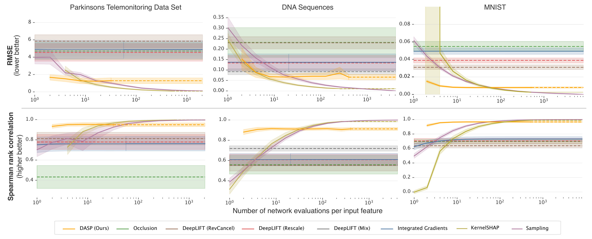 Figure 1
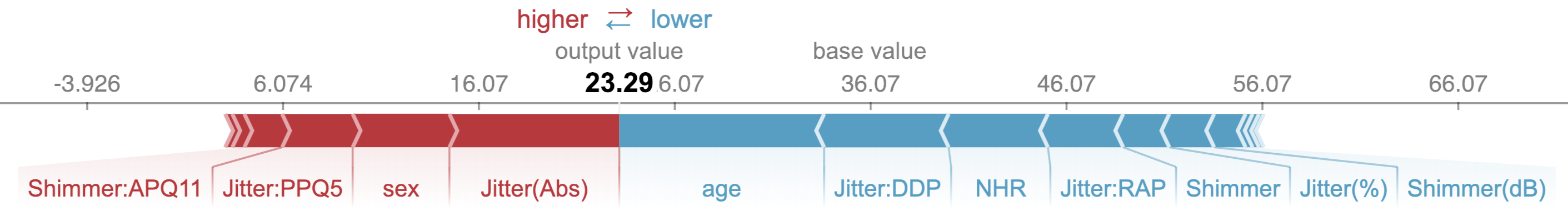 Figure 2
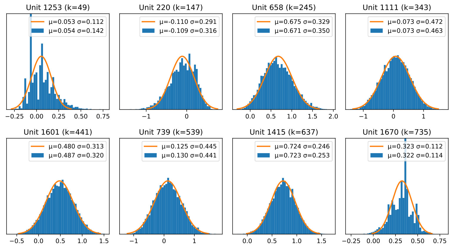 Figure 3
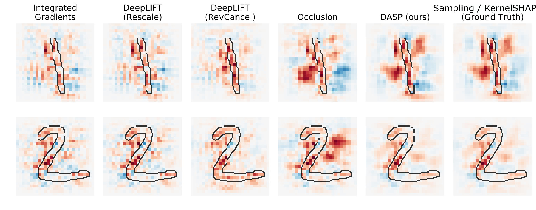 Figure 4
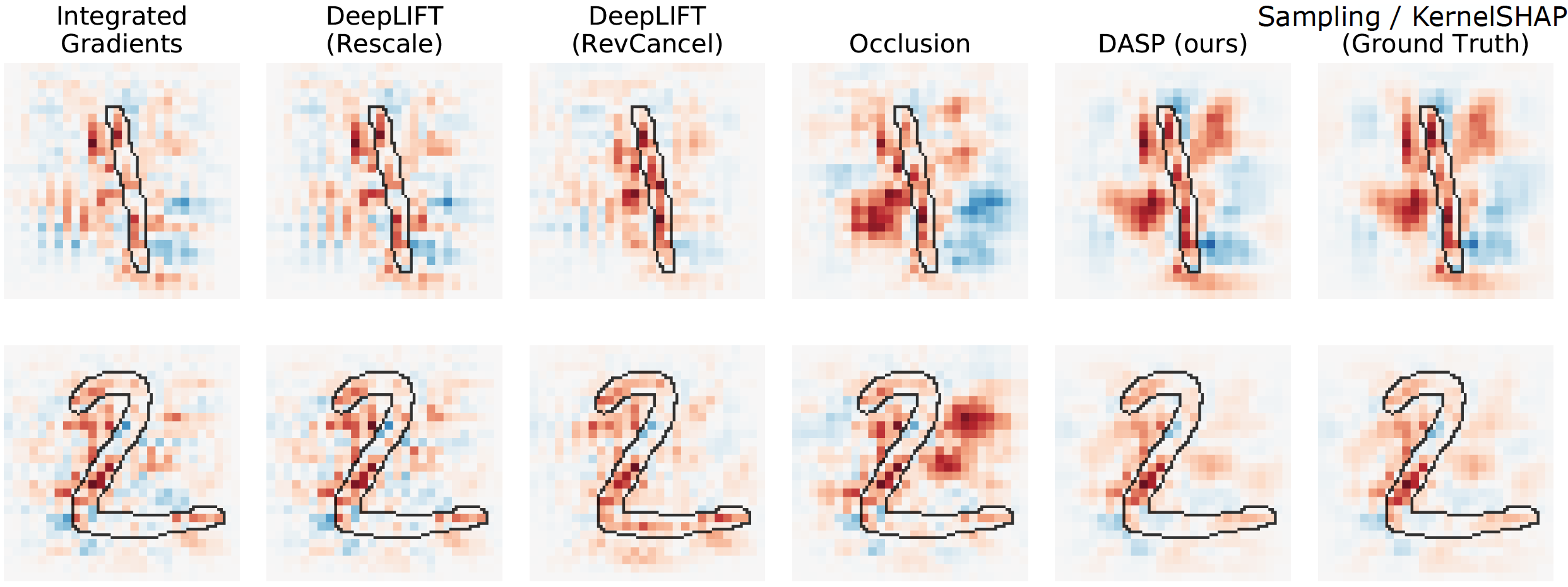 Figure 5
Peer Reviews
No public reviews on file for this paper yet. If you reviewed it on a platform where reviews are public (OpenReview, ICLR, NeurIPS, ICML), you can paste yours below so the community can read it here.
Code & Models
Videos
No videos yet. Explain this paper in a talk, walkthrough, or lecture? Add one.
Explaining Deep Neural Networks with a Polynomial Time Algorithm for Shapley Values Approximation
Marco Ancona
Cengiz Öztireli
Markus Gross
Abstract
The problem of explaining the behavior of deep neural networks has recently gained a lot of attention. While several attribution methods have been proposed, most come without strong theoretical foundations, which raises questions about their reliability. On the other hand, the literature on cooperative game theory suggests Shapley values as a unique way of assigning relevance scores such that certain desirable properties are satisfied. Unfortunately, the exact evaluation of Shapley values is prohibitively expensive, exponential in the number of input features. In this work, by leveraging recent results on uncertainty propagation, we propose a novel, polynomial-time approximation of Shapley values in deep neural networks. We show that our method produces significantly better approximations of Shapley values than existing state-of-the-art attribution methods.
Neural Networks, Attribution methods, Shapley values, Explainable AI, XAI
RNN Recurrent Neural Network GRU gated recurrent unit LSTM long short-term memory MFCC Mel-frequency cepstral coefficient PEM per-epoch noise mixing SNR signal-to-noise ratio ASR automatic speech recognition CNN Convolutional Neural Network DNN Deep Neural Network ACCAN accordion annealing WSJ Wall Street Journal CTC Connectionist Temporal Classification WFST Weighted Finite State Transducer WER word error rate CER character error rate LVCSR large-vocabulary continuous speech recognition ROI range of interest STAN sensor transformation attention network SER sequence error rate HMM Hidden Markov Model LER label error rate NN Neural Networks MLP Multilayer Perceptron ReLU Rectified Linear Unit PCC Pearson correlation coefficient LPN Lightweight Probabilistic Deep Network
1 Introduction
Deep Neural Networks have demonstrated enormous potential in solving a variety of problems, growing the sophistication and impact of machine learning. On the other hand, while machine learning models are being employed on an increasing number of fields, the black-box nature of DNNs is still a barrier to the adoption of these systems for those tasks where interpretability is a requirement. Recently, European regulators introduced the legal notion of a right to explanation (Goodman & Flaxman, 2016), demanding transparency for any automated decision having a deep impact on the life of the people involved, which affects the adoption of black-box models like DNNs on some domains.
Since the notion of interpretability is complex, multi-faceted and not yet fully defined (Doshi-Velez & Kim, 2017; Lipton, 2016), several works have focused on investigating methods for local interpretability. Contrarily to global interpretability, which aims at explaining the general model behavior, local interpretability scope is restricted at explaining a particular decision for a given model and input instance (Doshi-Velez & Kim, 2017).
In the realm of local interpretability, attribution methods have received particular attention in the last years (Ras et al., 2018). Consider a model that takes an N-dimensional input and produces a C-dimensional output , like a DNN with output neurons. Depending on the application, the input features can have a different nature, like pixels for images or components of a multi-dimensional word vector representation for natural language processing. Similarly, each output of the network can represent either a numerical predicted quantity (regression task) or the probability of a corresponding class (classification task).
Formally, attribution methods aim at producing explanations by assigning a scalar attribution value, sometimes also called “relevance” (Bach et al., 2015) or “contribution” (Shrikumar et al., 2017), to each input feature of a network for a given input sample. In particular, for a single target output indexed with , the goal of an attribution method is to determine the contribution of each input feature to the output . For clarity of notation, in the remainder of the paper, we will simply use whenever possible. For a classification task, the target output can be chosen to be the one associated with the highest output probability (to understand which part of the input was mostly relevant for the prediction) or the one associated with a different class (to assess whether the input contains evidence that supports or rejects a different class). Over the last decade, several attribution methods have been specifically developed for neural networks (Simonyan et al., 2014; Zeiler & Fergus, 2014; Springenberg et al., 2014; Bach et al., 2015; Ribeiro et al., 2016; Selvaraju et al., 2016; Shrikumar et al., 2017; Sundararajan et al., 2017; Montavon et al., 2017; Zintgraf et al., 2017; Lundberg & Lee, 2017; Kindermans et al., 2018).
When an explanation is generated, it should be a natural requirement to have a clear understanding of how the explanation method works, a condition necessary to make sure the explanation itself is a reliable and unbiased representation of the network behavior. In fact, some recent works showed that attribution methods can actually produce unreliable or misleading results, despite these being visually appealing to humans (Kindermans et al., 2017; Ghorbani et al., 2019; Adebayo et al., 2018; Nie et al., 2018). This problem is fueled by the limited theoretical understanding of some of these methods and lack of reliable quantitative metrics to evaluate explanations in the absence of a ground-truth (Adebayo et al., 2018). To overcome these limitations, some authors have recently endorsed an axiomatic approach (Sun & Sundararajan, 2011; Sundararajan et al., 2017; Montavon et al., 2017; Lundberg & Lee, 2017; Kindermans et al., 2017). In this context, an axiom is a self-evident property of the attribution method that should be satisfied for any explanation generated by the method itself. By leveraging these properties, attribution methods with stronger theoretical guarantees can be designed (Sundararajan et al., 2017).
Along with this research direction, the literature on cooperative game theory suggests Shapley values (Shapley, 1953) as a unique way of assigning attributions such that certain desirable axioms are satisfied. Shapley values are a classic game theory solution for the distribution of credits to players participating in a cooperative game. Notably, the unique set of properties of Shapley values, discussed in the next section, seems to fit naturally in the setting of attributions as well (Strumbelj & Kononenko, 2010; Sun & Sundararajan, 2011; Datta et al., 2016; Lundberg & Lee, 2017).
On the other hand, computing the exact Shapley value is, in general, NP-hard (Matsui & Matsui, 2001) and only feasible for less than 20-25 players (i.e. input features for our case). Some previous works proposed sampling-based methods to approximate Shapley values (Castro et al., 2009; Strumbelj & Kononenko, 2010; Datta et al., 2016). While these methods are unbiased estimators, as the number of input features grows they require thousands of model evaluations, which is expensive for DNNs. KernelSHAP (Lundberg & Lee, 2017) combines sampling with lasso regression to reduce the number of samples but it also introduces a bias from the regularizer. Other fast approximations designed for DNNs exist but these are based on the strong assumptions of model linearity (Lundberg & Lee, 2017). At the best of our knowledge, there is no exhaustive evaluation of the empirical accuracy of these methods as Shapley value approximators in DNNs.
The contribution of this work is threefold: 1) endorsing an axiomatic approach, we compare Shapley values to existing state-of-the-art attribution methods, motivating the use of the former to explain non-linear models; 2) we formulate a novel, polynomial-time approximation of Shapley values specifically designed for DNNs; 3) we assess empirically the approximation power of our algorithm compared to other attribution methods on three datasets and architectures.
2 Attribution Methods
Attribution methods can be partitioned into two broad categories: backpropagation-based methods and perturbation-based methods (Ancona et al., 2018). In this section, we define Shapley values and briefly review some popular attribution methods that will be later used in our experimental comparison. We focus on methods that can be applied to a variety of architectures and that are not restricted to some particular input type (eg. images).
2.1 Backpropagation-based methods
Methods in this category compute attributions running only one or a few backward passes through the network. Many such methods have been proposed in the last years. The prototypical example is Saliency maps (Simonyan et al., 2014) where attributions are computed as the absolute gradient of the target output with respect to each input feature. Gradient Input (Shrikumar et al., 2016) introduces an element-wise multiplication between the input and the (signed) gradient, producing more sharp results:
[TABLE]
While the gradient provides information about which features can be locally perturbed the least in order for the output to change the most, applied to a highly non-linear function only provides local information and it does not help to compute the marginal contribution of a feature. To overcome this limitation, other methods have been proposed such as Layer-wise Relevance Propagation (LRP) in several variants (Bach et al., 2015; Montavon et al., 2017), DeepLIFT (in its two variants, Rescale and RevealCancel) (Shrikumar et al., 2016, 2017), and Integrated Gradients (Sundararajan et al., 2017). Compared to Gradient Input, these methods are characterized by different propagation rules for non-linear operations in the network than the instant gradient. In the case of Integrated Gradients, DeepLIFT Rescale, and -LRP, the propagation rule can be seen as computing a form of average gradient (Ancona et al., 2018). In the other cases, the propagation rule is designed on specific heuristics.
2.2 Perturbation-based methods
This category includes methods that estimate the contribution of input features by removing or perturbing them and measuring the variation of the network target output as a consequence of this operation (Ribeiro et al., 2016; Zintgraf et al., 2017; Fong & Vedaldi, 2017). The simplest perturbation method computes attributions by setting each feature sequentially to zero (Zeiler & Fergus, 2014):
[TABLE]
In the remainder of the paper, we will refer to this method simply as “Occlusion”.
Remark Notice that the procedure of replacing features with a zero value implicitly defines a baseline that can be used to indicate features that are toggled off. Many attribution methods require the definition of a baseline to indicate the absence of information. This is further discussed in Appendix C of the supplementary material.
Most often perturbation-based methods are simple to implement but very slow, as several evaluations of the network are necessary. Additionally, the number of features perturbed at each iteration and the choice of the perturbation itself are hyper-parameters of these methods that can heavily affect the resulting explanations, making it difficult to interpret the results (Ancona et al., 2018).
2.3 Shapley values
Shapley values can be considered a particular example of perturbation-based methods where no hyper-parameters, except the baseline, are required.
Consider a set of players and a function that maps each subset of players to real numbers, modeling the outcome of a game when players in participate in it. The Shapley value is one way to quantify the total contribution of each player to the result of the game when all players participate. For a given player , it can be computed as follows:
[TABLE]
The Shapley value for player defined above can be interpreted as the average marginal contribution of player to all possible coalitions that can be formed without it.
While is a set function, the definition can be adapted for a neural network function by defining a baseline as discussed above. Then we can replace in Eq. 3 with , where indicates the original input vector where all features not in are replaced with the baseline value.
It has been observed (Lundberg & Lee, 2017) that attributions based on Shapley values better agree with the human intuition empirically. Unfortunately, computing Shapley values exactly requires us to evaluate all possible feature subsets as in Eq. 3. This is clearly prohibitive for more than a couple of dozens of variables.
For certain simple functions , it is possible to compute Shapley values exactly in polynomial time. For example, the Shapley values of the inputs to a max-pooling layer can be computed with function evaluations (Lundberg & Lee, 2017). When this is not possible, Shapley values sampling (Castro et al., 2009) can be used to estimate approximate Shapley values based on sampling of Eq. 3. For specific games, other approximate methods have been developed. In particular, (Fatima et al., 2008) proposed a polynomial time approximation for weighted voting games (Osborne & Rubinstein, 1994) based on the idea that, instead of enumerating all coalitions, it might suffice to estimate their expected contributions. The same idea is used as the first step of our approximation algorithm for deep neural networks in Sec. 4. Before going into the details of the derivations, we present a review of theoretical properties of Shapley values and other attribution methods.
3 Axiomatic comparison of attribution methods
We start our theoretical analysis by observing the following connection between existing attribution methods and Shapley values for linear models.
Proposition 1**.**
Occlusion, Gradient Input, Integrated Gradients and DeepLIFT produce exact Shapley values when applied to a linear model and a zero baseline is used.
The proof (provided in Appendix A of the supplementary material) comes directly from the observation that all these methods are equivalent for linear models (Ancona et al., 2018). For non-linear models, instead, these methods produce different attributions. DeepLIFT RevealCancel (Shrikumar et al., 2017) and its variant DeepSHAP (Lundberg & Lee, 2017) approximate Shapley values at each layer independently and use the chain rule to compose these into attributions. Unfortunately, the chain rule does not hold in general for Shapley values. Integrated Gradients (Sundararajan et al., 2017), on the other hand, can be shown to compute Aumann-Shapley values (Aumann & Shapley, 1974), an extension of Shapley values for infinite games where each individual player has a negligible contribution. While this method has better theoretical properties, it is not yet clear how well these assumptions apply to real scenarios where the number of input features is limited and the individual features may have a significant impact.
In order to better understand the relations among methods and their advantages, it is essential to evaluate them with respect to desirable theoretical properties. We thus compare different attribution methods according to the following axioms already established in the literature: (1) conservation, (2) null player, (3) symmetry, (4) linearity, (5) continuity and (6) implementation invariance.
Axiom 1: Completeness. An attribution method satisfies completeness when attributions sum up to the difference between the value of the function evaluated at the input, and the value of the function evaluated at the baseline, i.e. . This property, also called efficiency (Shapley, 1953), summation to delta (Shrikumar et al., 2017) or conservation (Montavon et al., 2017), has been recognized by previous works as desirable to ensure the attribution method is comprehensive in its accounting.
Axiom 2: Null player. If the function implemented by a DNN does not depend on some variable, then the attribution to that variable should always be zero.
Axiom 3: Symmetry. If the function implemented by a DNN depends on two variables and but not on their order (i.e. ), then the attribution assigned to these variables should be the same every time the input and the baseline provides the same values for these variables. This axiom, also called anonymity (Sun & Sundararajan, 2011), is arguably a desirable property for any attribution method: if two variables play the exact same role in the DNN, they should receive the same attribution.
Axiom 4: Linearity. If the function implemented by a DNN can be seen as a linear combination of the functions of two sub-networks (i.e. ), then any attribution should also be a linear combination, with the same weights, of the attributions computed on the sub-networks, i.e. , where denotes the attributions for the DNN that implements the function . Intuitively, this is justified by the need for preserving linearities within the network (Sundararajan et al., 2017).
Axiom 5: Continuity Attributions generated for two nearly identical inputs should be nearly identical, i.e. . This axiom assumes the attribution is generated for a continuous prediction function , which is always the case for DNNs built by combining continuous functions. In this case, the prediction for two nearly identical inputs is also nearly identical, which motivates a nearly identical explanation (Montavon et al., 2017).
Axiom 6: Implementation Invariance. Two networks are said to be functionally equivalent if their outputs are equal for all inputs, despite having (possibly very) different implementations (Sundararajan et al., 2017). Attribution methods should produce identical results when applied to any functionally equivalent network provided with the same input. The importance of this property relies on the observation that any explanation should only depend on the input and the function implemented by the DNN, not its implementation. This property is satisfied by all perturbation-based methods (that only relies on the function evaluation) as well as by all backpropagation-based methods relying purely on the gradient (which is itself implementation-invariant). This axiom was proposed in a previous work (Sundararajan et al., 2017) where it is shown that it can be violated when other propagation rules are used, like in DeepLIFT and LRP.
It is trivial to see that Gradient Input and Occlusion do not satisfy Completeness, while it has been showed that LRP and DeepLIFT do not satisfy Implementation Invariance (Sundararajan et al., 2017). Instead, the following notable result can be shown for Shapley values.
Proposition 2**.**
Shapley values is the only possible attribution method that satisfies Axioms 1-5.
The proposition is a direct consequence of previous results (Sun & Sundararajan, 2011) and the proof is provided in Appendix B of the supplementary material. Clearly, being a perturbation-based method, Shapley values satisfies Axiom 6 as well. This unique set of sought after properties motivates the use of Shapley values for attributions.
4 Deep Approximate Shapley Propagation
Despite the theoretical guarantees, Shapley values have one big flaw: computing them is NP-hard, as elaborated on in the previous sections. In this section, we introduce Deep Approximate Shapley Propagation (DASP), a perturbation-based method that can reliably approximate Shapley values in DNNs with a polynomial number of perturbation steps.
Consider a feed-forward neural network, composed of layers equipped with a non-linear function , each performing
[TABLE]
where indicates a layer index, .
We are interested in computing the Shapley values with respect to one output unit of a neural network whose overall function is the composition of several of such layers.
Our approximation is based on the following intuition. According to the definition given by Eq. 3, the Shapley value of an input feature is given by its marginal contribution to all possible coalitions that can be made out of the remaining features. Since we are interested in an average value, we can compute the expected contribution to a random coalition instead of enumerating each of them. In particular, we consider the distribution of coalitions of size , for each , that do not include the feature , and compute the expected contribution of that feature with respect to these distributions. The average of all these marginal contributions gives the feature’s approximate Shapley value (Fatima et al., 2008):
[TABLE]
where the expectations are over the distribution of sets of size , and denotes the contribution of feature to any random coalition of size . More explicitly, we can write the expected contribution of a feature for a given coalition size as the expected target output difference with and without it, i.e.
[TABLE]
The proof of Eq. 5 is based on the observation that there exists the same number of coalitions (where order matters) of size for all values of . We refer the reader to (Fatima et al., 2008) for the complete derivation.
So the main problem is approximating these expected values for all coalitions of size . As we will elaborate on in the next sections, these expected values can be computed and propagated along with variances from layer to layer in a DNN. Such a propagation can be achieved by transforming the architecture of a given DNN to replace the point activations at all layers by probability distributions. This problem has been previously studied in the scope of uncertainty propagation in DNNs (Abdelaziz et al., 2015; Gast & Roth, 2018; Thiagarajan et al., 2018), where the goal is to analyze how the uncertainty of the input data or of the network parameters propagates through the linear and non-linear operations up to the output layer. We adapt such a framework for our use case by i) considering the network parameters fixed and hence no source of uncertainty, and ii) introducing input uncertainty based on sampling of input coalitions. Then, we employ a Lightweight Probabilistic Network (Gast & Roth, 2018), and show that the expected values can be propagated in a practical fashion through the entire network.
4.1 Input distribution from random coalitions
Each coalition of size is represented with a vector of inputs, where the set of components of the vector contain their actual values, and the others contain the baseline value of zero. All such vectors with non-zero elements can be thought of as drawn from an underlying distribution of a random variable .
The first operation in a typical DNN is a weighted sum of the inputs. Each hidden unit thus takes a weighted sum of the network input . As is a random variable, a weighted sum of its components is also a random variable. It can be shown (Von Bahr, 1972) that, under mild assumptions, the distribution of is given by
[TABLE]
where we set
[TABLE]
with the sums computed over all components of the input vector . We provide a study of the accuracy of this form of the distribution by comparing it to the empirical counterpart in Appendix D of the supplementary material.
The random vector with the components is thus distributed with an isotropic Gaussian of the means and variances . Note that if we assume that this weighted sum is the only layer in the network, then the means here already provide the expected values we need to compute Shapley values. As this random variable is fed into the further operations of the later layers in a DNN, the distribution and hence the means will change. The next task is thus to derive how the distribution of will change as it is fed through.
4.2 Distribution propagation
Given the probabilistic input at the first hidden layer, we propagate this distribution to the target unit by employing Lightweight Probabilistic Deep Networks (Gast & Roth, 2018). LPN is an architecture for uncertainty propagation through a feed-forward DNN where each input sample is modeled using an independent univariate Gaussian distribution. Contrary to other Bayesian formulations, the model parameters are considered deterministic, as in our case. The propagation of uncertainties is carried out using assumed density filtering (Boyen & Koller, 1998; Gast & Roth, 2018), where each layer is implemented as filtering of the input distribution to obtain a transformed Gaussian distribution with diagonal covariance. While it was originally developed to propagate the intrinsic uncertainty of the input, LPN can be easily adapted to our scenario, where the uncertainty given by random coalitions induces a probability distribution for the input of the first hidden layer. On the other hand, notice that DASP is not coupled to any particular probabilistic framework and can extend to general architectures (eg. RNNs) given a probabilistic framework that supports them.
In order to propagate the activation distribution through linear and non-linear operations, LPN converts any layer with point activations into an uncertainty propagation layer by matching first and second-order central moments, i.e.
[TABLE]
where and denote expectation and variance. This procedure can be proven to perform a greedy (layer-wise) optimization of the KL-divergence of towards the actual distribution (Minka, 2001). As a result, our original network function is transformed into a probabilistic network function that takes as inputs the first and second moments of a (Gaussian) distribution and returns the parameters of the distribution at the output layer, after the original distribution is sequentially filtered by all hidden layers. Moment matching for several commonly employed layers and operations in neural network architectures can be derived in closed-form:
Affine transformation. A fully-connected layer with weights and bias takes the input and filters it by applying . The output is a new Gaussian with mean and variance:
[TABLE]
where by we indicate the element-wise square. This notation will be used for any matrix or vector in the remainder of the paper. With minor adaptations, this also holds for the convolution and the mean pooling, which are linear layers. Notice that mean and variance do not interact with each other on linear operations.
ReLU activation. The output of a ReLU activation that receives a Gaussian input is a rectified Gaussian distribution (Socci et al., 1998) whose mean and variance can be derived analytically (Frey & Hinton, 1999). For details, see Appendix E of the supplementary material.
Max Pooling. Max pooling can be seen as returning the maximum response of random variables . For two independent inputs , , the maximum is not normally distributed anymore. Nevertheless, it has been shown that the univariate normal is an effective approximation (Gast & Roth, 2018) and the first and second moments, provided also in Appendix E, can be derived analytically (Jacobs & Berkelaar, 2000).
4.3 Computing approximate Shapley values
Having transformed the distribution of inputs from coalitions to output activation uncertainties, we can finally compute approximate Shapley values. Algorithm 1 describes the procedure in pseudo-code. For the sake of clarity, we have listed all the operations of the first weighted sum as explained in Sec. 4.1 explicitly, and wrapped all other operations in subsequent layers into .
Computing Deep Shapley values requires network evaluations for each input feature, if we test all possible coalition sizes (i.e. ). As a result, the algorithm approximates Shapley values for input features in network evaluations, compared to of the exact computation. In order to further reduce the computational cost, we can perform a secondary approximation by reducing the number of coalition sizes that we consider. If is the number of coalition sizes tested, we need evaluations. In the next section, we show empirically that can be much lower than . In order to ensure as much diversity as possible, we pick coalition sizes equally apart from each other.
5 Experiments
In this section, we report experiments running DASP111DASP implementation: http://bit.ly/DASPCode alongside Integrated Gradients, DeepLIFT Rescale, DeepLIFT, RevealCancel, Occlusion, Shapley sampling and KernelSHAP using three datasets and different network architectures. Instead, we omit the comparison with DeepSHAP as this method is equivalent to DeepLIFT Rescale when used with a (fixed) zero baseline. Our main goal is to demonstrate how DASP can be effectively used to approximate Shapley values and compare it with state-of-the-art attribution methods on this task. Notice that Shapley sampling and KernelSHAP (without regularizer) are guaranteed to converge to exact Shapley values, given enough samples. This is not the case for DASP, which is not a sampling-based method. In this case, our goal is to show that sampling-based methods require significantly more model evaluations than DASP to reach the same approximation error.
All experiments are run in Keras (Chollet et al., 2015). Details about the architectures used are in Appendix F of the supplementary material.
5.1 Evaluation metrics
When the size of the input allows it, we compute exact Shapley values using Eq. 3, and use it as the ground-truth. When the exact computation is not feasible, we run Shapley sampling until convergence as an approximation of the ground-truth. Since Shapley sampling is an unbiased estimator, this is a faithful approximation.
For the quantitative comparison, we report both the root mean squared error (RMSE) and the Spearman rank correlation over several input samples extracted from each test set. While the RMSE is useful to quantify the absolute average error of each attribution score, the Spearman rank correlation is used as a metric to assess whether two methods agree on the ranking of features based on their impact on the model output. When discussing performance, we always compare the attribution methods by the number of network evaluations they require, as the wall-clock time is influenced by the efficiency of the different implementations. However, we do take into account that our probabilistic layers require about twice the number of operations of a normal layer (to propagate mean and variance), therefore we double the number of evaluations for DASP in all our results.
5.2 Parkinsons disability assessment
As a first test, we trained a fully-connected DNN on the Parkinsons Telemonitoring Data Set (Tsanas et al., 2010). The goal of this regression task is to predict the Parkinson’s disease rating scale (UPDRS) that reflects the presence and severity of symptoms starting from 18 input features: subject age, subject gender, and 16 biomedical voice measures. UPDRS spans the range 0-176, with 0 representing healthy state and 176 representing total disabilities.
Fig. 2 shows the explanation of the network prediction generated by our method for a single subject. An explanation, in this case, can tell the user which features the model has used for a certain prediction. The natural question is whether the generated explanation is a reliable representation of the network behavior. Notice that the network behavior and the human intuition about how a certain task should be solved might not coincide in general (for example, the network might have learned patterns that the human expert was not aware of, or the network might mistakenly exploit correlations that have no causality). For this reason, we believe any qualitative comparison is dangerous. Instead, we have a clear ground truth against which we can evaluate our technique and others in this case. As the number of input features is limited to 18, we can compute the exact Shapley values for 100 samples from the test set, each requiring network evaluations. Fig. 1 shows that DASP produces a better approximation of Shapley values than other biased methods, even when a small number of coalition sizes is tested (i.e. ). Unbiased, sampling-based methods, instead, require significantly more evaluations before outperforming DASP.
5.3 Classifying regulatory DNA sequences
To test if the result holds on different architectures, we consider a classification task over DNA sequence inputs. A DNA sequence can be seen as a string over the alphabet A,C,G,T. We are interested in detecting short patterns (eg. GATAA or GATTA) within these sequences by employing a neural network with two 1D convolutional layers, global average pooling, and one fully-connected layer. This setup, which also includes some synthetically generated DNA sequences, was previously proposed as a benchmark for attribution methods (Shrikumar et al., 2017). Since the DNA sequences have a length of 200 tokens, it is prohibitive to compute exact Shapley values. To approximate the ground-truth and enable a direct comparison of all methods against it, we run about 800’000 iterations of Shapley sampling on each of the 50 input samples until convergence. This process took about 45 minutes on our machine.
The results are reported in Fig. 1. The original authors of the experiment suggest a specific combination of DeepLIFT propagation rules (Rescale for the two convolutional layers and RevealCancel for the dense layer) to obtain the best results on this dataset. This combination, identified as DeepLIFT (Mix) in Fig. 1, also gives the best results among backpropagation-based methods in our experiment, outperformed only by DASP and sampling methods. On the other hand, KernelSHAP requires a significantly more evaluations than DASP to reach the same rank correlation.
5.4 Digits classification (MNIST)
Finally, we train a convolutional neural network on MNIST (LeCun et al., 1998) to perform digit classification. We use the LeNet-5 architecture (LeCun et al., 1998), which consists of two convolutional layers, each followed by a max-pooling layer, and three final dense layers. Again, we use Shapley sampling to approximate the ground-truth for the 784 features (pixels) of 50 test images, which took about 4 hours for 6M evaluations on our machine.
Fig. 3 shows an example of the resulting attribution maps. Notice that backpropagation-based methods tend to produce more noisy explanations than perturbation-based methods. We speculate that this happens because backpropagation-based methods are more sensitive to local (and noisy) gradient information. Furthermore, Occlusion seems to under-estimate or over-estimate the importance of some areas of the image, as compared to DASP. These are reflected in the quantitative comparison in Fig. 1. As in the previous experiments, we see a significant gap between the accuracy of DASP and other biased approximators, as well as a significant gap in the number of samples required by Shapley sampling and KernelSHAP to reach DASP performance. Notice that, in this case, KernelSHAP performs worse than simple sampling. We speculate this happens because of the linearity assumption of KernelSHAP, affecting more the more complex models.
6 Conclusions
In this work, we discussed Shapley values as an attribution method for DNNs. First, we showed that several existing attribution methods reduce to computing Shapley values when applied to linear models. On the other hand, when the model is non-linear, Shapley values remain the only method that satisfies a number of desirable theoretical properties, which strongly motivates their use for reliable explanations.
As computing Shapley values is often unfeasible, we then proposed Deep Approximate Shapley Propagation (DASP), a novel perturbation-based method that approximates Shapley values using uncertainty propagation in DNNs. DASP requires a polynomial number of network evaluations. While it is not guarantee to recover exact Shapley values, we showed empirically that other sampling-based methods require significantly more evaluations to achieve the same approximation error. We have also shown that DASP outperforms state-of-the-art backpropagation-based methods, which are fast but coarse Shapley values approximators.
DASP can be considered a novel application for the field of uncertainty propagation in DNNs, although we would like to remark how it is not constrained to LPN for this purpose. As research on this area continues, we expect to be able to extend DASP for recurrent neural networks, and we hope that new probabilistic frameworks will enable the derivation of theoretical guarantees and even better approximations.
The reference list from the paper itself. Each links out to its DOI / PubMed record.
- 1Abdelaziz et al. (2015) Abdelaziz, A. H., Watanabe, S., Hershey, J. R., Vincent, E., and Kolossa, D. Uncertainty propagation through deep neural networks. In Interspeech 2015 , 2015.
- 2Adebayo et al. (2018) Adebayo, J., Gilmer, J., Muelly, M., Goodfellow, I., Hardt, M., and Kim, B. Sanity checks for saliency maps. In Advances in Neural Information Processing Systems , pp. 9524–9535, 2018.
- 3Ancona et al. (2018) Ancona, M., Ceolini, E., Oztireli, C., and Gross, M. Towards better understanding of gradient-based attribution methods for deep neural networks. In 6th International Conference on Learning Representations (ICLR 2018) , 2018.
- 4Aumann & Shapley (1974) Aumann, R. J. and Shapley, L. S. Values of non-atomic games . Princeton University Press, 1974.
- 5Bach et al. (2015) Bach, S., Binder, A., Montavon, G., Klauschen, F., Müller, K.-R., and Samek, W. On pixel-wise explanations for non-linear classifier decisions by layer-wise relevance propagation. Plo S one , 10(7):e 0130140, 2015.
- 6Boyen & Koller (1998) Boyen, X. and Koller, D. Tractable inference for complex stochastic processes. In Proceedings of the Fourteenth Conference on Uncertainty in Artificial Intelligence , UAI’98, pp. 33–42, San Francisco, CA, USA, 1998. Morgan Kaufmann Publishers Inc. ISBN 1-55860-555-X.
- 7Castro et al. (2009) Castro, J., Gamez, D., and Tejada, J. Polynomial calculation of the shapley value based on sampling. Computers and Operations Research , 36(5):1726 – 1730, 2009. ISSN 0305-0548. doi: https://doi.org/10.1016/j.cor.2008.04.004 . Selected papers presented at the Tenth International Symposium on Locational Decisions (ISOLDE X).
- 8Chollet et al. (2015) Chollet, F. et al. Keras. https://keras.io , 2015.
