Non-asymptotic error controlled sparse high dimensional precision matrix estimation
Adam B Kashlak

TL;DR
This paper introduces a new method for estimating sparse high-dimensional precision matrices that controls false positive rates with finite sample guarantees, applicable to Gaussian networks and genomics.
Contribution
A novel distribution-free methodology for precision matrix estimation that explicitly controls false positive rates in high-dimensional settings.
Findings
Method achieves finite sample guarantees for false positive control.
Applicable to Gaussian graphical models and gene network inference.
Performs well in high-dimensional, sparse settings.
Abstract
Estimation of a high dimensional precision matrix is a critical problem to many areas of statistics including Gaussian graphical models and inference on high dimensional data. Working under the structural assumption of sparsity, we propose a novel methodology for estimating such matrices while controlling the false positive rate, percentage of matrix entries incorrectly chosen to be non-zero. We specifically focus on false positive rates tending towards zero with finite sample guarantees. This methodology is distribution free, but is particularly applicable to the problem of Gaussian network recovery. We also consider applications to constructing gene networks in genomics data.
Click any figure to enlarge with its caption.
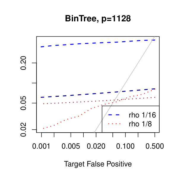 Figure 1
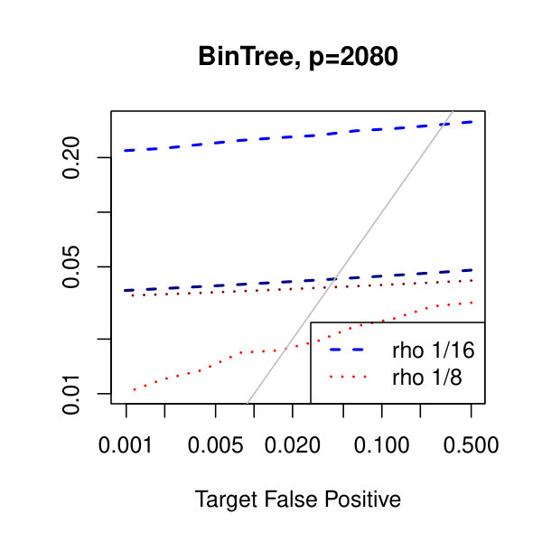 Figure 2
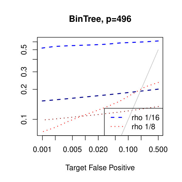 Figure 3
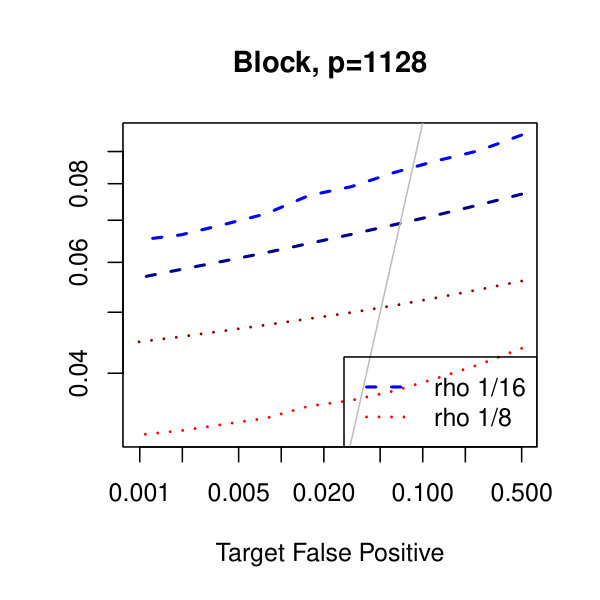 Figure 4
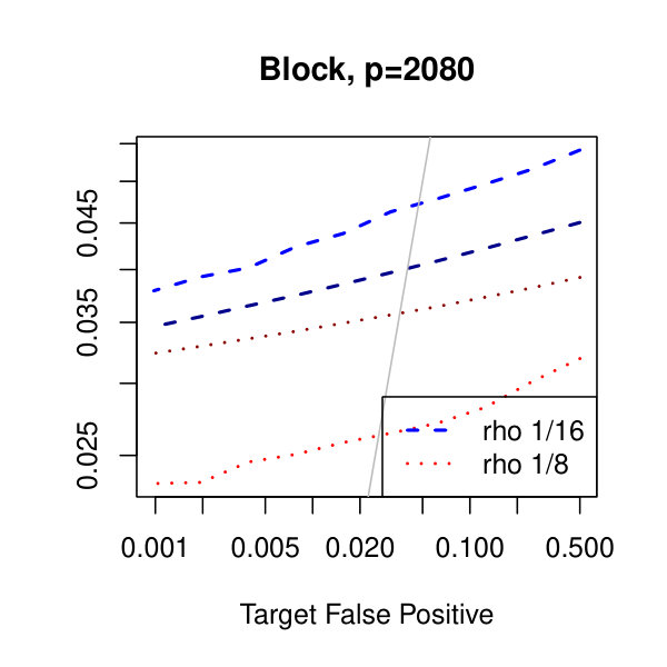 Figure 5
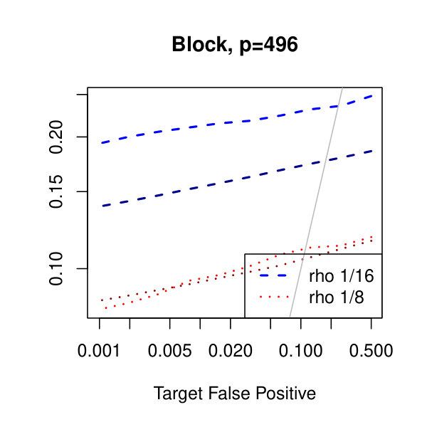 Figure 6
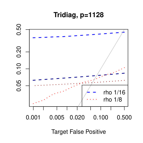 Figure 7
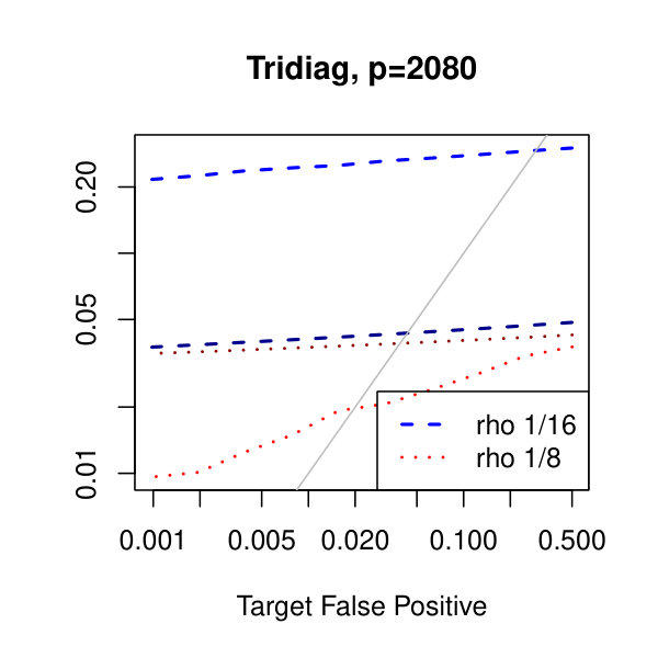 Figure 8
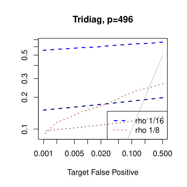 Figure 9
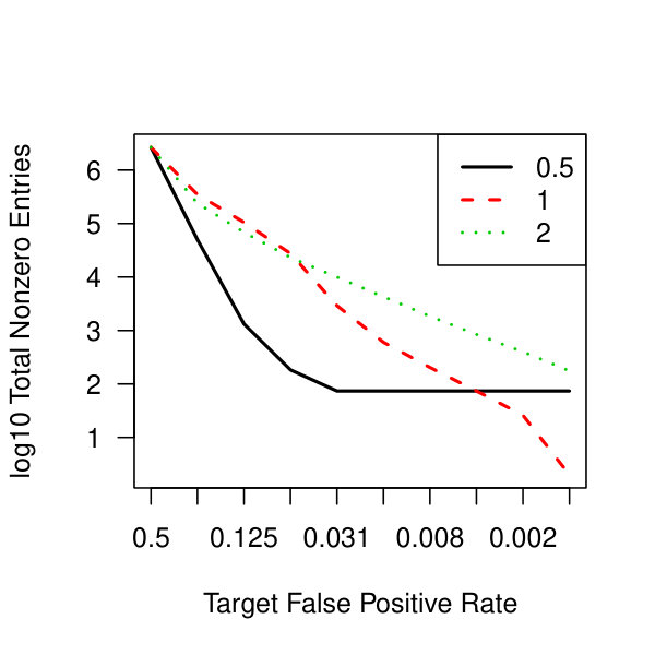 Figure 10
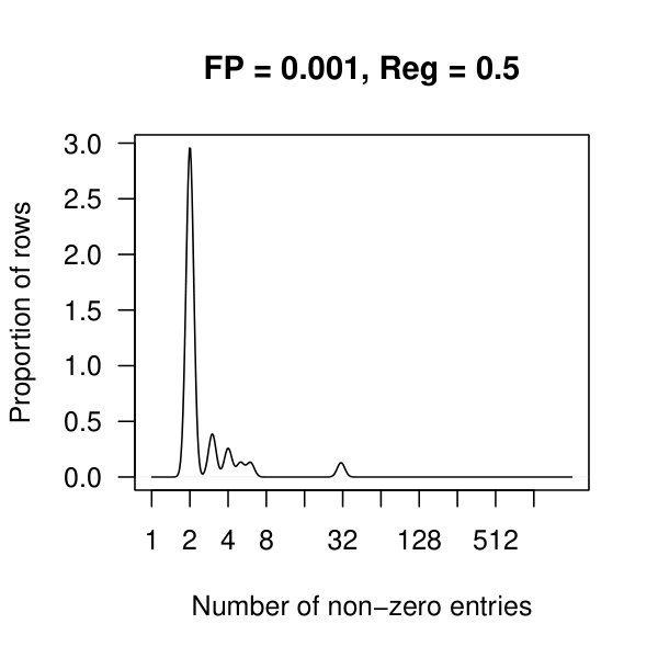 Figure 11
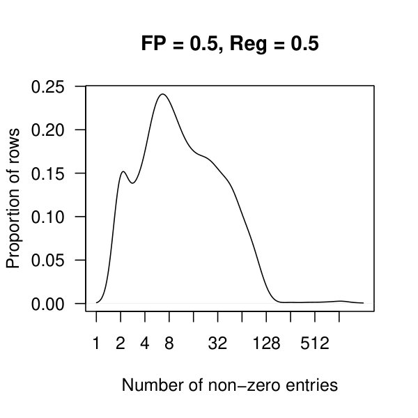 Figure 12
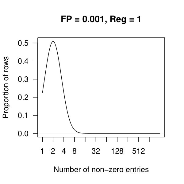 Figure 13
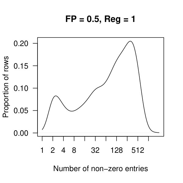 Figure 14
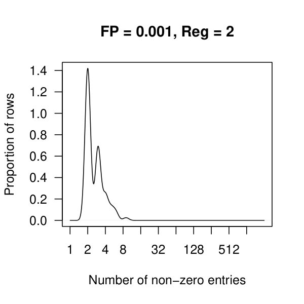 Figure 15
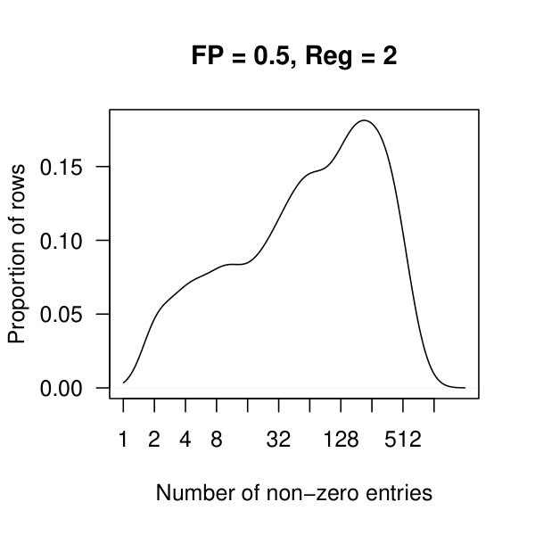 Figure 16
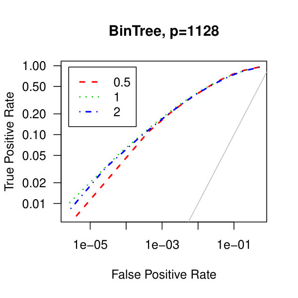 Figure 17
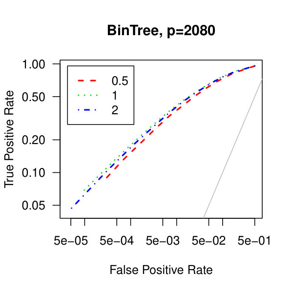 Figure 18
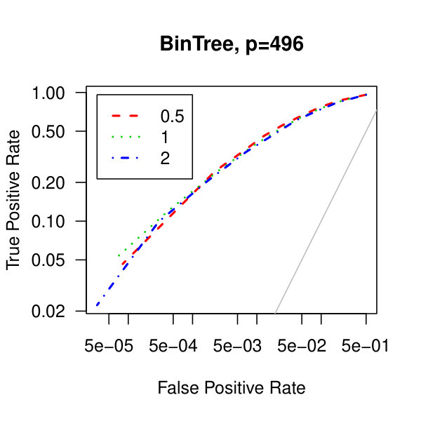 Figure 19
 Figure 20
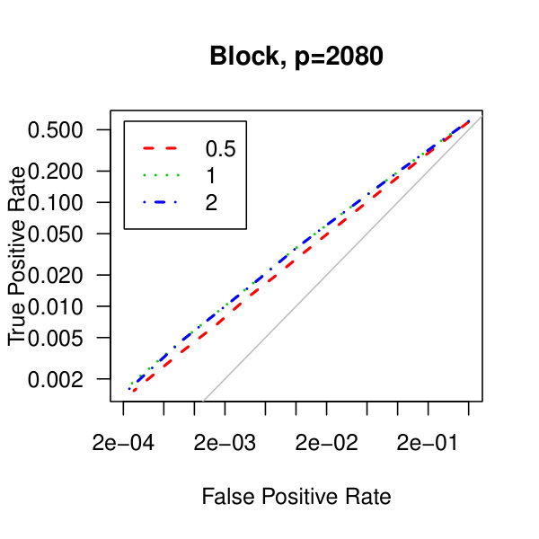 Figure 21
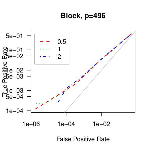 Figure 22
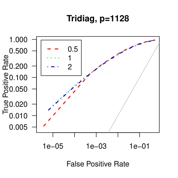 Figure 23
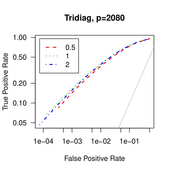 Figure 24
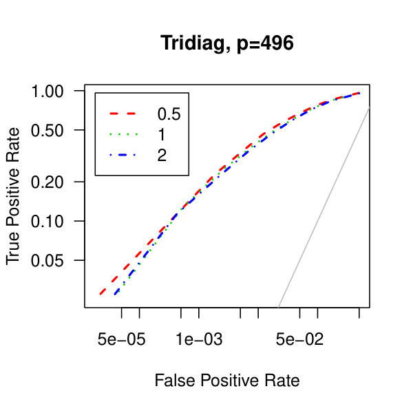 Figure 25
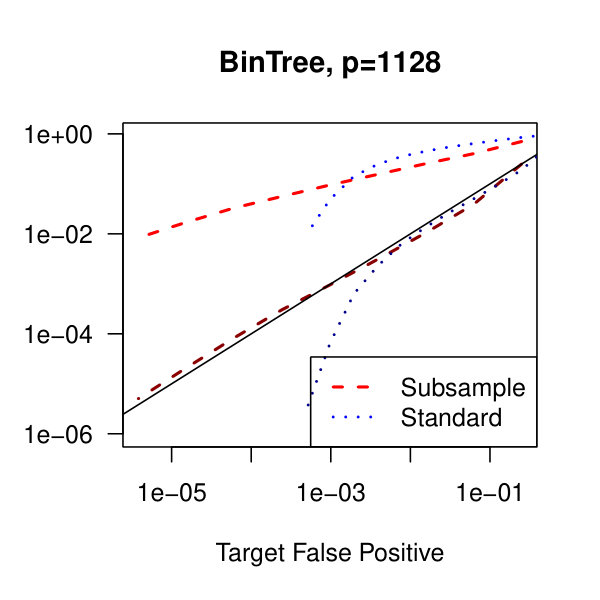 Figure 26
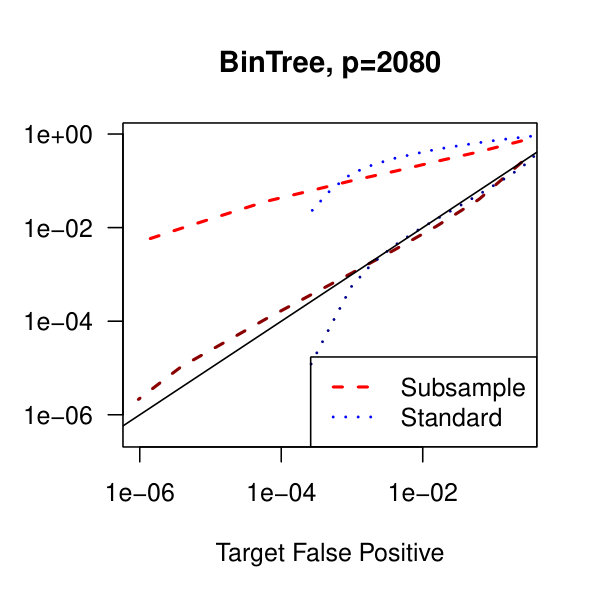 Figure 27
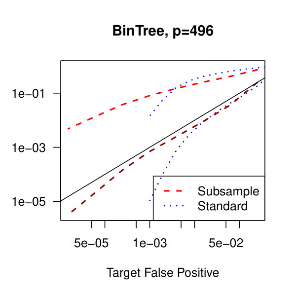 Figure 28
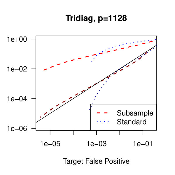 Figure 29
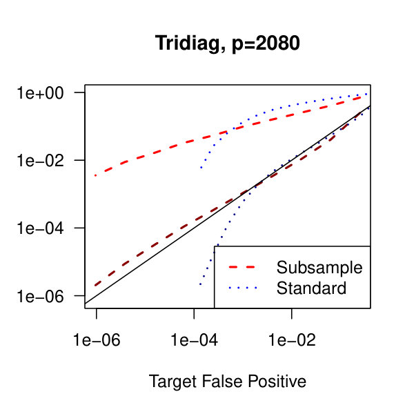 Figure 30
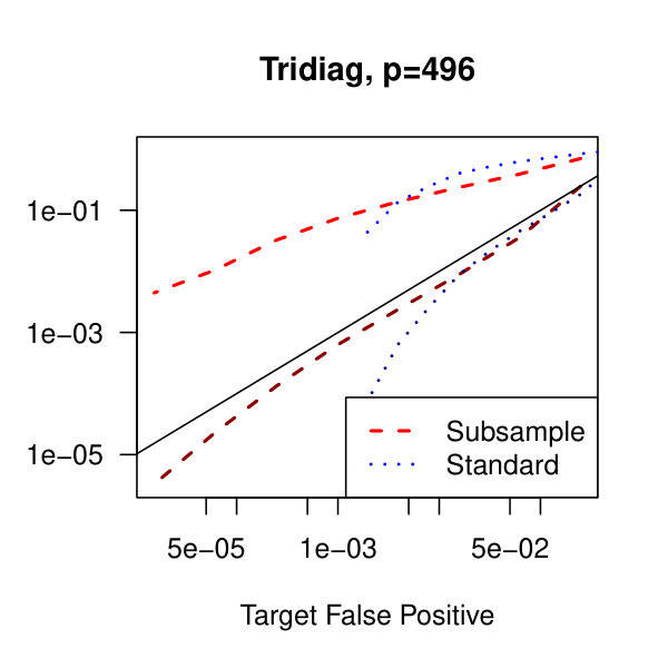 Figure 31
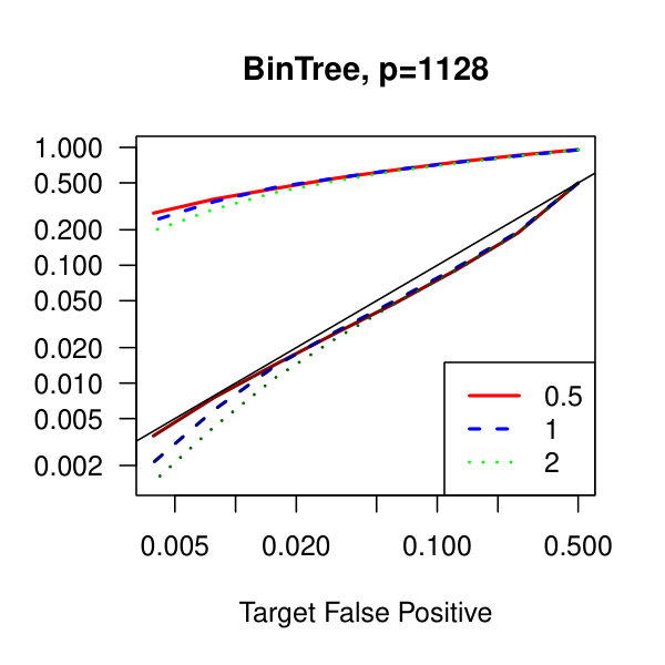 Figure 32
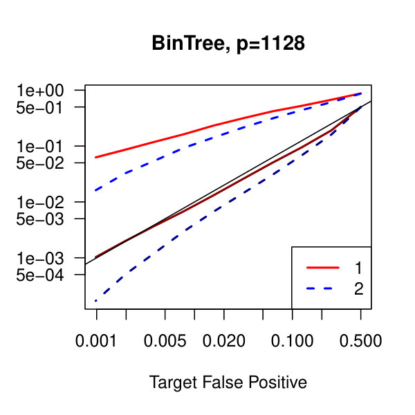 Figure 33
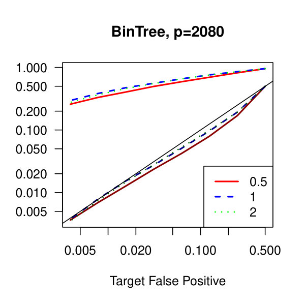 Figure 34
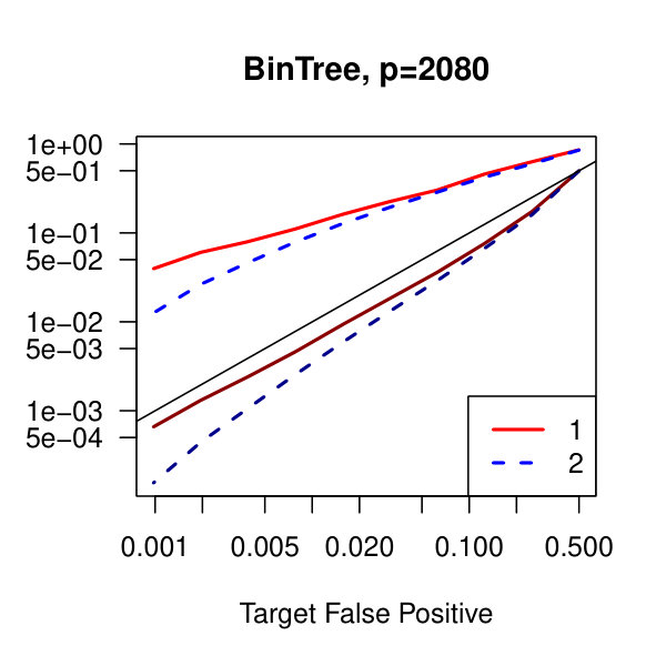 Figure 35
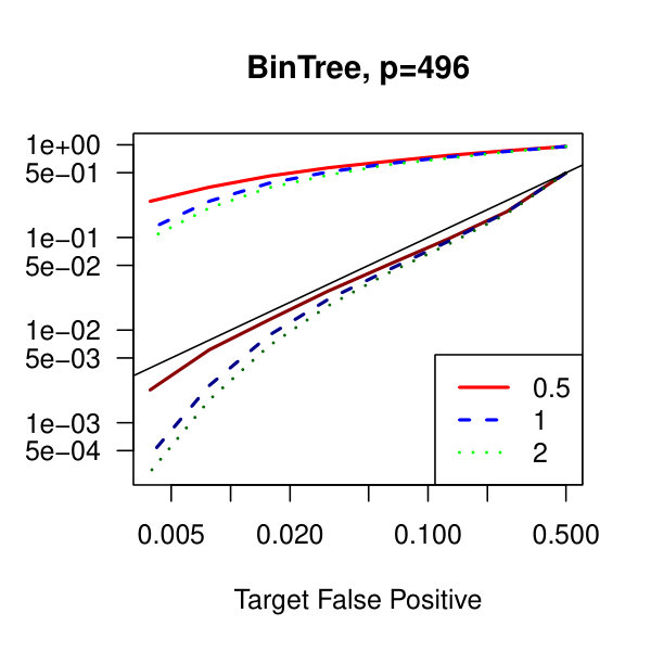 Figure 36
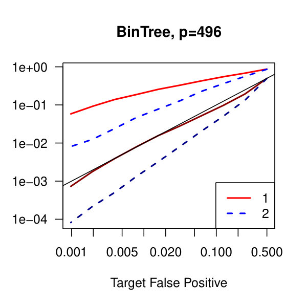 Figure 37
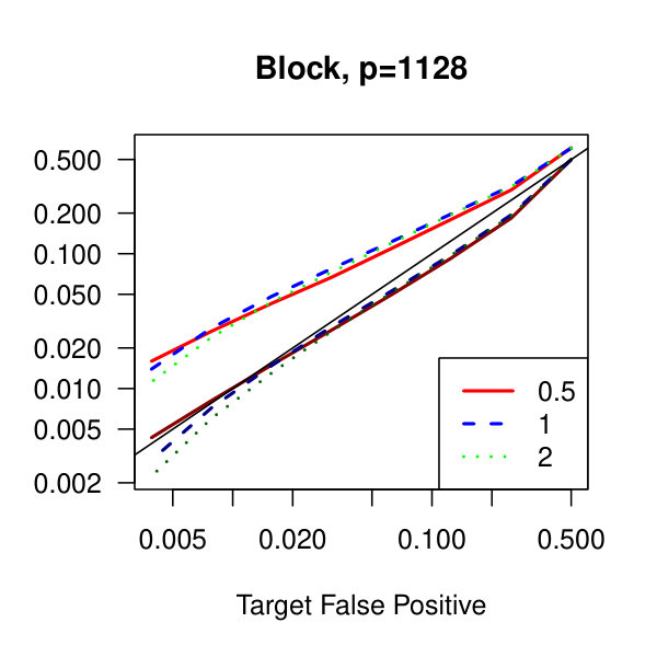 Figure 38
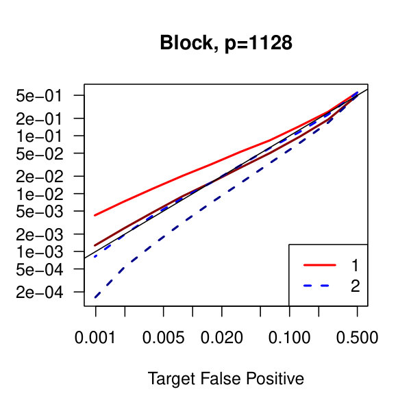 Figure 39
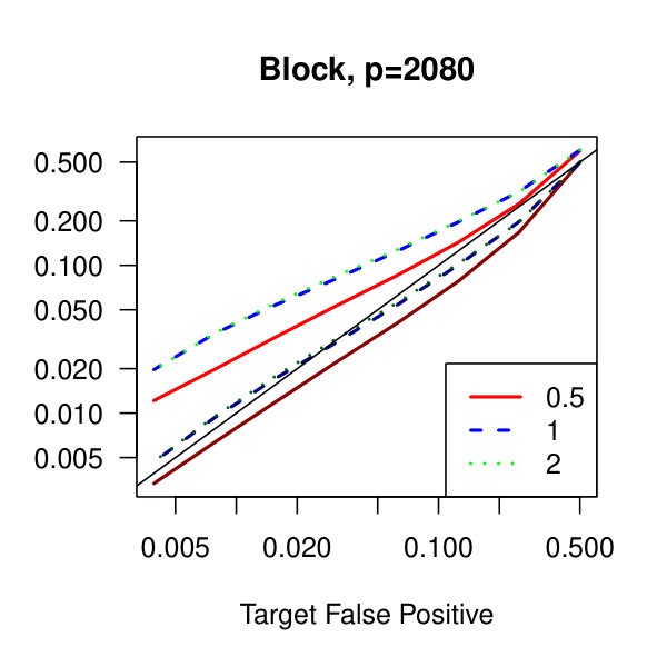 Figure 40
Peer Reviews
No public reviews on file for this paper yet. If you reviewed it on a platform where reviews are public (OpenReview, ICLR, NeurIPS, ICML), you can paste yours below so the community can read it here.
Videos
No videos yet. Explain this paper in a talk, walkthrough, or lecture? Add one.
Non-asymptotic error controlled sparse high dimensional
precision matrix estimation
Adam B Kashlak
Mathematical & Statistical Sciences
University of Alberta
Edmonton, Canada, T6G 2G1
Abstract
Estimation of a high dimensional precision matrix is a critical problem to many areas of statistics including Gaussian graphical models and inference on high dimensional data. Working under the structural assumption of sparsity, we propose a novel methodology for estimating such matrices while controlling the false positive rate–percentage of matrix entries incorrectly chosen to be non-zero. We specifically focus on false positive rates tending towards zero with finite sample guarantees. This methodology is distribution free, but is particularly applicable to the problem of Gaussian network recovery. We also consider applications to constructing gene networks in genomics data.
1 Introduction
Attempting to estimate the graphical structure of a high dimensional network is problemsome when edges are rare but the number of nodes is large. In standard statistical classification problems, we fix a palatable false positive rate and aim to recover as many true positives as possible. Thus, we treat support recovery as a binary classification problem. For nodes, the number of potential edges to consider is on the order of . With a sample size , there are too many parameters to accurately estimate. However, when trying to classify edges as significant or not under the assumption of sparsity, the assumption that most edges are not significant, if we have even a small false positive rate, then this will result in many erroneous connections potentially obscuring follow up research. For example, a genomics study considering the conditional correlation structure of, say, 2000 genes will have to consider over two million potential edges. A standard 1% false positive rate will result in tens of thousands of erroneous connections.
To address this issue, we consider the extreme estimation setting of recovering the support of a precision matrix in the high dimensional setting, , assuming belongs to a class of sparse positive definite matrices, and for false positive rates . Making use of debiased estimators (Bühlmann, 2013; Javanmard & Montanari, 2014; Van de Geer et al., 2014; Jankova & Van De Geer, 2015), the non-asymptotic results of Kashlak & Kong (2017), and a clever subsampling methodology, we can achieve finite sample guarantees in this extreme setting.
There has been much past work on covariance and precision matrix estimation much of which is summarized in the survey Fan et al. (2016). Most estimators for high dimensional precision matrices are based on penalization including the graphical lasso (Friedman et al., 2008), the CLIME and ACLIME estimators (Cai et al., 2011, 2016), and the debiased estimator of Jankova & Van De Geer (2015) used for constructing confidence sets and running hypothesis tests. These articles all rely on high dimensional asymptotics, which is that estimation is successful in the limit as and grow to infinity together generally such that , or some variant thereof, is . Our work differs as it considers guaranteed results for controlling the support recovery of as the false positive rate for fixed finite , which is asymptotic in , a controllable tuning parameter, instead of in and , which are generally fixed in the real world experimental setting.
Our method can be deconstructed into two steps. The first is to find a bias-corrected initial estimate for the precision matrix . The second is to construct a ball in the operator norm topology corresponding to the target false positive rate and then search this ball for a sparse estimator. In actuality, given a false positive rate of , we step down in a binary fashion constructing successive false positive rates of and a sequence of estimators tending towards one with the desired . Depending on the sample size, we can randomly partition our data set into smaller sets, apply this two-step procedure to each subsample in parallel, and combine the results for improved performance. In step two, we use a binary search procedure which converges rapidly minimizing the computational burden.
Our search methodology is effectively a method for controlled thesholding of the initial debiased estimator. The literature on thresholding for precision matrices is quite light when compared to thresholding covariance matrices (Bickel & Levina, 2008a, b; Rothman et al., 2009; Cai & Liu, 2011; Kashlak & Kong, 2017). The challenge is that unlike the unbiased empirical covariance estimator, there is no unbiased empirical precision estimator. Debiasing such precision matrix estimators allows for thresholding as mentioned in Jankova & Van De Geer (2015). Furthermore, Jankova & Van De Geer (2015) proposed an entrywise thresholding method given some false positive rate , which while working well in some high dimensional asymptotic sense, proved to not achieve the target false positive rate on simulated data.
2 Methodology
2.1 Notation
In this article, we primarily make use of the family of Schatten norms. For with th entry and eigenvalues , we define the trace norm , the Hilbert-Schmidt norm and the operator norm . We will also use the standard norms applied to vectors in and entrywise to matrices in .
The algorithm in Section 2.3 makes use of hard thresholding. For , we define the hard thresholding operator , which returns a matrix with th entry
[TABLE]
which simply removes entries from with magnitude less than .
2.2 Initial Estimator
Let be an independent and identically distributed collection of mean zero random vectors with common unknown positive definite covariance matrix and corresponding precision matrix . Of course, we require the covariance and its inverse to exist, but put no further assumptions on the distribution of the at the moment except to assume that is sparse. Specifically,
[TABLE]
where is the class of sparse matrices with no more than entries in each row or column non-zero and with non-zero entries bounded away from zero allowing them to be detectable. In practice, we attempt to recover the support of the normalized matrix with diagonal entries of 1 to avoid scale issues.
Our approach is similar to Kashlak & Kong (2017) who attempt to recover the support of a covariance matrix by starting with an initial estimator, constructing a confidence ball, and searching this ball for a sparser estimator. However, whereas this preceding work can use the empirical estimator, , as an unbiased initial estimator for controlled thresholding, we cannot construct an unbiased estimator for the precision matrix in the setting.
A standard estimator for sparse precision matrices is the graphical lasso (Friedman et al., 2008), which is based on an penalized maximum likelihood under the Gaussian distribution:
[TABLE]
for some tuning parameter . The graphical lasso is debiased in Jankova & Van De Geer (2015), which uses a correction factor based on the subgradient of the above optimization extending the work of Van de Geer et al. (2014) that debiases the classic lasso estimator for linear regression. The resulting debiased estimator is
[TABLE]
Alternatively, the CLIME method (Cai et al., 2011) solves a constrained optimization problem to find .
[TABLE]
with a more sophisticated version ACLIME (Cai et al., 2016) adapting to individual entries.
A different regularized estimator is the ridge estimator,
[TABLE]
whose closed form solution is . Consider the singular value decomposition where , , and for . In Bühlmann (2013), a bias corrected estimator for ridge regression is proposed. This is achieved by finding some other estimator, which is used to correct for the projection bias. We can apply the same method to the ridge precision matrix estimator to get
[TABLE]
where is some other estimate for and where is the projection in onto an dimensional subspace spanned by the columns of , and is that projection with the diagonal entries set to zero. Bühlmann (2013) uses the graphical lasso estimator for .
2.3 Binary Search
Given an initial estimator from the previous setting henceforth denoted for simplicity of notation and some such that for some positive integer corresponding to the number of iterates of the below algorithm, we aim to construct an estimator with false positive rate by carefully thresholding the entries in so that
[TABLE]
which is that the desired false positive rate is achieved. The two extreme estimators are the initial estimator and the diagonal matrix with diagonal entries coinciding with and off-diagonal entries set to zero. These correspond to the 100% and 0% false positive cases, respectively. For the remainder, we normalize to have unit diagonal thus making .
For values of tending towards zero, we consider the operator norm balls centred at being where refers to the operator norm for , which is the principal eigenvalue. This motivates the following algorithm:
Constructing an error controlled estimator
[TABLE]
In this algorithm, we quickly locate the densest estimator close to , alternatively being the sparsest estimator close to , by using a binary search procedure. Given the th iterated matrix as a starting point, we set the smallest half of the non-zero entries in magnitude in to zero, compute the distance to and then if the distance is greater than , we remove half of the remaining entries whereas if the distance is less than , we reintroduce half of the removed entries.
Remark 2.1**.**
For choice of and number of steps , values of closer to 1 result in smaller steps adding stability but requiring a larger to achieve a small false positive rate. In the simulations of Section 3.1, we use .
For the choice of initial estimator from Section 2.2, the best performance in simulated data experiments on multivariate normal data was achieved by beginning the above procedure with the debiased graphical lasso estimator of Jankova & Van De Geer (2015). This is mainly because their estimator follows the requirements of the theorems in the subsequent section as long as the data under analysis is sub-Gaussian. However, good performance is still observed when the data is sub-exponential as can be seen in the supplementary material.
Remark 2.2**.**
A similar search algorithm is proposed in Kashlak & Kong (2017). The main differences are that in the cited work, the operator norm balls are confidence sets centred about the empirical covariance estimator rather than centred about the identity matrix . Furthermore, the radii are reduced by a factor of in that previous work due to the low rank structure of the empirical covariance estimator. Specifically, rather than .
2.4 Theoretical Guarantees
The reason for shrinking the radius by in the above algorithm comes from applying tools from random matrix theory (Tao, 2012) to sparse matrices—see the supplementary material for proofs. The following result states that when is sufficiently sparse and , we can reduce the false positives by by shrinking the radius of an operator norm ball centred around the -dimensional identity matrix by .
Theorem 2.1** (Controlled False Positives).**
Let with for , and . For some false positive rate with , let the bias of the initial estimator be Then,
[TABLE]
Remark 2.3**.**
To control the false positive rate, we require a few assumptions in the theorem statement. Namely, the number of non-zero entries per row and the operator norm of cannot grow at a rate faster than as increases. In the simulations of Section 3.1, we have the much nicer setting where these quantities remain bounded as increases.
Remark 2.4**.**
The accuracy of the conclusion of Theorem 2.1 is improved as increases for a fixed sample size . This fact motivates the subsampling methodology in Section 2.5. Secondly, as the false positive rate decreases, the bias is allowed to be larger. Hence, we can choose based on . This is because as increases, we threshold more aggressively effectively fighting against increases in the bias.
As noted in Remark 2.1, we chose the method of Jankova & Van De Geer (2015) for our simulations in Section 3.1. It is shown in their work that this debiased estimator has the following maximal entrywise bias, or depending on specific assumptions on the sub-Gaussian nature of the data. Hence, . As we have control over the false positive rate , we can choose this to satisfy the conditions of the above theorem. Namely, considering false positive rates less than or , which are generally of more interest than large false positive rates.
Further considering the debiased estimator described in Jankova & Van De Geer (2015) and given the assumptions made in that article, we can recover the support of the matrix asymptotically as increase and . Indeed, Lemma 9 from Jankova & Van De Geer (2015) and equivalently Theorem 1 from Ravikumar et al. (2011) assume an irrepresentability condition common in the lasso literature and get convergence rates of the graphical lasso estimator depending on the tail behaviour of the random vectors . Thus, the graphical lasso estimator asymptotically recovers the support. Further assuming sub-Gaussian tails for the , Jankova & Van De Geer (2015) shows that the remainder term in the debiased graphical lasso estimator is asymptotically negligible. Thus, thresholding the debiased estimator will in turn re-recover the support. Similarly, the literature on sparse covariance matrix estimation generally requires sub-Gaussian tails for asymptotic support recovery (Bickel & Levina, 2008a, b; Rothman et al., 2009; Cai & Liu, 2011; Kashlak & Kong, 2017).
Beyond distributional assumptions, a quick calculation can demonstrate that the true positive probability is necessarily greater than the false positive probability. For some threshold corresponding to a false positive rate of , we have assuming symmetry of the distribution of that
[TABLE]
which is that the probability of a true positive at threshold corresponds to the probability of a false positive at threshold . Thus, this method is guaranteed to return at least as many true positives proportionally as false positives and generally, as will be seen in Section 3.1, performs much better.
2.5 Subsampling
As Theorem 2.1, becomes more accurate for large , we can run the above methodology in parallel by randomly partitioning the sample of size into subsamples of size . As a result, we run our method in parallel times returning estimators . For a false positive rate of and the assumption from Theorem 2.1 that with and , then the expected number of false positive recoveries is . After splitting the sample into disjoint pieces, we can run the above algorithm in parallel to construct independent estimators . The probability of recovering the same false positive entry in or more of the is a binomial tail sum: . When , then choosing is generally sufficient. Indeed, we can bound this binomial tail sum by the Kullback-Leibler divergence. For ,
[TABLE]
If we want a target false positive rate of , we can choose such that or to achieve the same false positive rate as when not subsampling. For example, if we take and keep , then we can relax the false positive rate for each individual subsampled estimator.
This addition of subsampling to the methodology allows for faster runtimes, as the estimators can be computed in parallel with fewer iterations, and also increases accuracy as the target false positive rate decreases below as will be seen in Section 3.1.
3 Applications
3.1 Simulated Data
We test our methodology for three different graphical structures. In the first case, tridiagonal–i.e. , if , if . This is the sparsest connected graph structure with edges on nodes. In the second case, represents a binary tree graph with depth resulting in nodes and edges, which is roughly edges for nodes. Similar to case one, diagonal entries are set to and non-zero off-diagonal entries are set to . In the third case, represents a disjoint collection of complete graphs on nodes. Thus, there are nodes and edges, and is a block diagonal matrix with blocks with being the matrix of all ’s and , the identity matrix.
For simulations, the sample size was fixed at . The dimensions considered are as they correspond to binary trees of depth , respectively, and correspond to block diagonal matrices with -blocks, respectively. In all nine cases considered, the non-zero off-diagonal entries are all set to with the diagonal entries set to .
In Figure 1, we plot the empirical true and false positive rates on the vertical axis against the target false positive rate on the horizontal axis. The target false positive rate acts as a tunable parameter. Three types of matrices, three dimensions, and three values of the graphical lasso regularization parameter are considered. Ideally, the observed false positive rates will be close to the solid black line, which is where the observed and target rates coincide. This occurs as the dimension increases in all three cases. For the sparser models–tridiagonal and binary tree structures–we are able to maintain a true positive rate above 20% as the false positive rate is taken to zero. Performance is much worse when trying to recover the block diagonal matrix. For the lowest dimension, , setting the penalization parameter gives the best results whereas in the higher dimensions gives the best performance albeit only slightly. Hence, it appears that for choosing an initial estimator, the graphical lasso penalization parameter can be set to regardless of dimension and true for this methodology. On this note, we also considered but the performance was terrible and thus it is not included in the figures. For an alternative look at the simulations, receiver operating characteristic curves are included in the supplementary material. The same simulations were also run on multivariate Laplace data with details in the supplementary material. In short, choosing allowed for the empirical false positive rate to stay close to the target rate whereas did not perform as well.
In Figure 2, we consider the tridiagonal and binary tree models estimated by the standard approach as before and by subsampling as in Section 2.5 with . By subsampling, we can extend the false positive rate from around , where the standard method begins to breakdown, all the way to around . Hence, we can have a controlled reduction in the empirical false positive rate to effectively zero, as the precision matrix only has entries, using the subsampling method.
In Table 1, we tabulate empirically achieved true and false positive rates from the cross validated graphical lasso (Friedman et al., 2018) and ACLIME estimators (Pang et al., 2016). These estimators were computed by splitting the sample in half and optimizing the tuning parameters with respect to the operator norm distance. The graphical lasso estimator’s achieved false positive was roughly halved as the dimension doubled. The ACLIME estimator much more aggressively penalized the matrix entries. The threshold method of Jankova & Van De Geer (2015) was also tested, which for a false positive rate , sets the individual entries in the debiased estimator to zero if
[TABLE]
where is the empirical covariance matrix and is the cumulative distribution function for the standard normal distribution. A figure in line with Figure 1 for this method is included in the supplementary material. In short, this approach should work asymptotically as . In our simulations, the empirically achieved false positive rate was not close to the target false positive rate.
3.2 Geonomics data
We apply our methodology to the dataset of gene expressions for a small round blue cell tumours mircoarray experiment from Khan et al. (2001), which is also analyzed in other works (Rothman et al., 2009; Cai & Liu, 2011). The data set consists of a training set of 64 vectors containing 2308 gene expressions. The data contains four types of tumours. Considering this , we construct error controlled precision matrix estimators using the algorithm from Section 2.3 choosing the debiased estimator of Jankova & Van De Geer (2015) as the initial estimator and for graphical lasso penalization parameter .
In Figure 3, we plot the cardinality of the support of the estimators for the three penalization parameters as the false positive rate ranges from to . For , the method plateaus quickly returning a small support of 74 nonzero off-diagonal entries. The other two lines continue to decay towards zero off-diagonal entries.
In Figure 4, we see kernel density plots of the number of non-zero entries per row aggregated over all 2308 rows. In these plots, and are considered. Comparing the top and bottom row of plots, we see that there are many rows with approx 500 nonzero entries when , which quickly drops to fewer than 10 nonzero entries per row once .
4 Supplementary Material
Supplementary material available at Biometrika online includes proofs for the main results and auxiliary results. Receiver operating characteristic curves for the data in Figure 1 are included, and additional simulations for exponential data and the method from Jankova & Van De Geer (2015) are also included.
5 Proofs
The theory behind the methodology in this article comes from redoing the results from random matrix theory, which generally achieves an operator norm of , under the assumption that only of the entries are non-zero. This gives similar results but with an operator norm of .
We first prove a lazy version of Hoeffding’s concentration inequality.
Lemma 5.1**.**
For some , let be independent mean zero random variables not necessarily equally distributed, and let also independent of the . Then,
[TABLE]
Proof.
The proof is more or less the same as that of the standard Hoeffding inequality. Without loss of generality, let . For any , we can bound the variance of by
[TABLE]
Thus, we have a bound on the cumulant generating function of that and Therefore, via Chernoff’s inequality, we have for any that
[TABLE]
Minimizing the righthand side over gives and finally that Running the proof for gives the reverse inequality. Combining those gives the desired result. Lastly, to adjust for , replace with in the above result. ∎
Using the lazy version of Hoeffding’s inequality, we can get concentration of the operator norm for a sparse random matrix using a modification of the standard -net argument as presented in Tao (2012) Section 2.3.
Theorem 5.1**.**
Let be a symmetric random matrix with entries , , and . Let be a symmetric Bernoulli random matrix with iid entries such that . If the lower triangular entries of are independent then,
[TABLE]
where denotes the entrywise or Hadamard product of and .
Proof.
For now, we consider and as iid ensembles—i.e. remove the and condition—and adjust for the symmetry at the end of the proof. Let . For any vector such that , we have that Therefore, from the proof of Lemma 5.1, independence of entries, and ,
[TABLE]
Thus, for any arbitrary unit vector , we can apply Lemma 5.1 to get
[TABLE]
To extend to , we construct a maximal -net of the unit sphere . That is, let be the maximal set of points in such that for any , . Let be the vector such that , which exists via compactness. Thus, there exists a such that as otherwise, the set would not be maximal. Furthermore, and thus . Therefore, by the union bound,
[TABLE]
From Lemma 2.3.4 of Tao (2012), for some absolute constant . Thus, for large enough, the righthand side becomes negligible.
Now, considering and symmetric with zero diagonal as in the theorem statement, we have that for and the strict lower and upper triangular portions of . Hence,
[TABLE]
∎
Remark 5.2**.**
The constants in the above proof are not necessarily optimal, but sufficient to justify our approach to controlled precision matrix estimation.
of Theorem 1.
For (a), has zero diagonal and off-diagonal entries bounded by two. Further, if , then . Hence, if , then so is . For the bias, let be a Bernoulli random matrix with probability that entry is 1. Then,
[TABLE]
Thus, we have by assumption and by applying theorem 5.1 as well as the Bai-Yin theorems in Tao (2012) Section 2.3 that
[TABLE]
and
[TABLE]
Therefore,
[TABLE]
For (b), let which is by the sparsity assumption.
[TABLE]
and similarly
[TABLE]
∎
6 Additional Simulations
6.1 Receiver operating characteristic curves
In Figure 5, we consider plots of the observed false positives against the observed true positives–that is, Receiver operating characteristic curves. Similarly to the analysis of Figure 1 from the main article,We see better performance for the tridiagonal and binary tree matrices than for the block diagonal matrix. Also, the graphical lasso penalization parameter does not have a large effect on the methodology. Though, perform marginally better than .
6.2 Sub-Exponential Data
The same simulations as in Section 3.1were rerun replacing the multivariate Gaussian distribution with the multivariate Laplace distribution, and are displayed in Figure 6. As expected, the true positive rate is not as large as in the Gaussian setting. When the penalization parameter for the graphical lasso is set to , we see that our methodology does not maintain the desired false positive rate as . However, for , the empirical false positive rate does approximately track with the desired false positive rate in the three simulation settings.
6.3 Asymptotic Threshold
In the work of Jankova & Van De Geer (2015), a thresholding method is proposed for the debiased graphical lasso estimator making use of the normal distribution function. Namely,
[TABLE]
where is the empirical covariance matrix and is the cumulative distribution function for the standard normal distribution. The same simulations as in Section 3.1 were run on this method for graphical lasso penalization parameters of . The larger values of resulted in all of the off-diagonal entries being set to zero. Hence, Figure 7 displays the false and true positive rates for only . This method should work asymptotically as . However, for our specific choices of and , this method failed to achieve anything close to the target false positive rate.
The reference list from the paper itself. Each links out to its DOI / PubMed record.
- 1Bickel & Levina (2008 a) Bickel, P. J. & Levina, E. (2008 a). Covariance regularization by thresholding. The Annals of Statistics , 2577–2604.
- 2Bickel & Levina (2008 b) Bickel, P. J. & Levina, E. (2008 b). Regularized estimation of large covariance matrices. The Annals of Statistics , 199–227.
- 3Bühlmann (2013) Bühlmann, P. (2013). Statistical significance in high-dimensional linear models. Bernoulli 19 , 1212–1242.
- 4Cai & Liu (2011) Cai, T. & Liu, W. (2011). Adaptive thresholding for sparse covariance matrix estimation. Journal of the American Statistical Association 106 , 672–684.
- 5Cai et al. (2011) Cai, T. , Liu, W. & Luo, X. (2011). A constrained ℓ 1 minimization approach to sparse precision matrix estimation. Journal of the American Statistical Association 106 , 594–607.
- 6Cai et al. (2016) Cai, T. , Liu, W. & Zhou, H. H. (2016). Estimating sparse precision matrix: Optimal rates of convergence and adaptive estimation. The Annals of Statistics 44 , 455–488.
- 7Fan et al. (2016) Fan, J. , Liao, Y. & Liu, H. (2016). An overview of the estimation of large covariance and precision matrices. The Econometrics Journal 19 , C 1–C 32.
- 8Friedman et al. (2008) Friedman, J. , Hastie, T. & Tibshirani, R. (2008). Sparse inverse covariance estimation with the graphical lasso. Biostatistics 9 , 432–441.