A splitting/polynomial chaos expansion approach for stochastic evolution equations
Andreas Kofler, Tijana Levajkovi\'c, Hermann Mena, Alexander, Ostermann

TL;DR
This paper introduces a novel approach combining splitting methods with polynomial chaos expansion to efficiently solve stochastic evolution equations, supported by convergence analysis and numerical validation.
Contribution
It develops a new method integrating deterministic splitting with polynomial chaos for stochastic PDEs, enhancing solution efficiency and accuracy.
Findings
Method effectively reduces stochastic PDEs to deterministic systems.
Convergence analysis confirms the method's reliability.
Numerical experiments validate the approach's accuracy.
Abstract
In this paper, we combine deterministic splitting methods with a polynomial chaos expansion method for solving stochastic parabolic evolution problems. The stochastic differential equation is reduced to a system of deterministic equations that we solve explicitly by splitting methods. The method can be applied to a wide class of problems where the related stochastic processes are given uniquely in terms of stochastic polynomials. A comprehensive convergence analysis is provided and numerical experiments validate our approach.
Click any figure to enlarge with its caption.
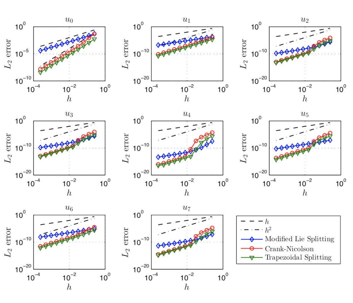 Figure 4
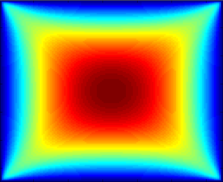 Figure 2
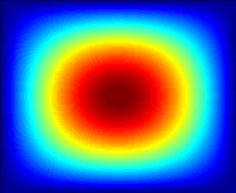 Figure 3
| CN | MLSPL | TSPL | |
|---|---|---|---|
| 0.0133 | 0.0373 | 0.0530 | |
| 0.0214 | 0.0241 | 0.0379 | |
| 0.1005 | 0.1008 | 0.0948 | |
| 0.4098 | 0.3652 | 0.4047 | |
| 2.7620 | 1.8051 | 1.8237 | |
| 41.1284 | 9.3921 | 13.5091 |
Peer Reviews
No public reviews on file for this paper yet. If you reviewed it on a platform where reviews are public (OpenReview, ICLR, NeurIPS, ICML), you can paste yours below so the community can read it here.
Videos
No videos yet. Explain this paper in a talk, walkthrough, or lecture? Add one.
\newunicodechar\textcommabelow
s\cbs
A splitting/polynomial chaos expansion approach for stochastic evolution equations
Andreas Kofler1, Tijana Levajković2,
Hermann Mena3 and Alexander Ostermann4
Abstract.
In this paper we combine deterministic splitting methods with a polynomial chaos expansion method for solving stochastic parabolic evolution problems. The stochastic differential equation is reduced to a system of deterministic equations that we solve explicitly by splitting methods. The method can be applied to a wide class of problems where the related stochastic processes are given uniquely in terms of stochastic polynomials. A comprehensive convergence analysis is provided and numerical experiments validate our approach.
Key words and phrases:
Splitting methods, Polynomial chaos expansion.
2000 Mathematics Subject Classification:
60H15, 65J10, 60H40, 60H35, 65M75, 11B83
1Andreas KOFLER, Department of Radiology, Charité-Universitätsmedizin Berlin, Germany, [email protected]
2Tijana LEVAJKOVIĆ, Institute of Stochastics and Business Mathematics, Vienna University of Technology, Austria, [email protected]
3Hermann MENA, Department of Mathematics, Yachay Tech University, Urcuquí, Ecuador, [email protected] & Department of Mathematics, University of Innsbruck, Austria, [email protected]
4Alexander OSTERMANN, Department of Mathematics, University of Innsbruck, Austria, [email protected]
1. Introduction
Splitting methods are numerical methods for solving differential equations, both ordinary and partial differential equations (PDEs), involving operators that are decomposable into a sum of (differential) operators. These methods are used to improve the speed of calculations for problems involving decomposable operators and to solve multidimensional PDEs by reducing them to a sum of one-dimensional problems [10]. Splitting methods have been successfully applied to many types of PDEs, e.g. [14], [16]. Exponential splitting methods are applied in cases when the explicit solution of a splitted equation can be computed. Such computations often rely on applying fast Fourier techniques, see for instant [38]. Resolvent splitting is used in cases when the splitted equation cannot be solved explicitly [17], [34]; here we consider this type of methods.
There are also many results in the literature about the approximation of solutions of SPDEs using splitting methods, see e.g. [2], [3], [4], [5], [9], [12], [15] and references therein. In [12] a splitting method for nonlinear stochastic equations of Schrödinger type is proposed. There the authors approximate the solution of the problem by a sequence of solutions of two types of equations: one without stochastic term and other containing only the stochastic term. They prove that an appropriate combination of the solutions of these equations converges strongly to the solution of the original problem. Exponential integrators for nonlinear Schrödinger equations with white noise dispersion were proposed in [5]. For a stochastic incompressible time-dependent Stokes equation different time-splitting methods were studied in [4]. In [2] the convergence of a Douglas–Rachford type splitting algorithm is presented for general SPDEs driven by linear multiplicative noise. In this work a splitting/polynomial chaos expansion is considered for stochastic evolution equations. Our approach has not been considered in the literature for solving these types of SPDEs so far.
We consider stochastic evolution equations of the form
[TABLE]
where , and are differential operators acting on Hilbert space valued stochastic processes, is a cylindrical Brownian motion on a given probability space and and are deterministic functions. In [30] equation (1.1) involving Gaussian noise terms was solved in an appropriate weighted Wiener chaos space. The deterministic problem that corresponds to (1.1), i.e., the case where and , for particular , and was studied in [10]. We consider equation (1.1) involving a non-Gaussian noise term. Namely, we consider inhomogeneous parabolic evolution equations involving the operators that can be split in and uniformly distributed random inputs. These equations, can be also written in the form
[TABLE]
where represents the noise term, see e.g. [20], [25], [28], [29], [30]. The existence of a random parameter is due to uncertainties coming from initial conditions and/or a random force term. Therefore, the solution is considered to be a stochastic process.
Stochastic processes with finite second moments on white noise spaces can be represented in series expansion form in terms of a family of orthogonal stochastic polynomials. The classes of orthogonal polynomials are chosen depending on the underlying probability measure [19], [20]. Namely, the Askey scheme of hypergeometric orthogonal polynomials and the Sheffer system [36], [37] can be used to define several discrete and continuous distribution types [39]. For example, in the case of the Gaussian measure, the orthogonal basis of the space of random variables with finite second moments is constructed by the use of the Hermite polynomials. We consider problems with non-Gaussian random inputs. The noise term is considered to be uniformly distributed. It is known that in order to obtain a square integrable solution of (1.1) with deterministic initial condition, it is enough to assume that the operator is elliptic and that the stochastic part (the noise term) is sufficiently regular, see e.g. [8]. In this work, the assumptions on the input data for problem (1.2) will be set such that the existence of a square integrable solution is always established. We do not consider solutions which are generalized stochastic processes as in [28], [30], since our focus is on numerical treatment.
Our approach is general enough to be applied to problems with additive noise, problems involving multiplicative noise and problems with convolution-type noise [28]. For instance, with this approach the heat equation with random potential, the heat equation in random (inhomogeneous and anisotropic) media and the Langevin equation can be solved. If (1.1) does have a sufficiently regular solution, this solution can be projected on an orthonormal basis in some Hilbert space, resulting in a system of equations for the corresponding Fourier coefficients. Thus, we use the so-called polynomial chaos method or the chaos expansion method and define the solution of (1.1) as a formal Fourier series with the coefficients computed by solving the corresponding system of deterministic PDEs [30]. With this method, the deterministic part of a solution is separated from its random part. Particularly, in the case of Gaussian noise, the orthonormal basis of stochastic polynomials involves the Hermite polynomials and in the case when the noise term is uniformly distributed, the orthonormal basis involves the Legendre polynomials [36]. By construction, the solution is strong in the probabilistic sense. It is uniquely determined by the coefficients, free terms, initial condition and the noise term. The coefficients in the Fourier series are uniquely determined by equation (1.1) and are computed by solving (numerically) the corresponding lower-triangular system of deterministic parabolic equations. The polynomial chaos method has been successfully applied for solving general classes of SPDEs. The list of references is long, here we mention just a few [20], [28], [32], [33]. In [25], [26], [27] this approach has been recently applied to the stochastic optimal regulator control problem [13].
Practical application of the Wiener polynomial chaos involves two truncations, truncation with respect to the number of the random variables and truncation with respect to the order of the orthogonal Askey polynomials used (in the particular case considered, the Legendre polynomials), see e.g. [21].
The paper is organized as follows. In Section 2 we introduce the notation and basic concepts used in the following sections. In Section 3 we present the splitting/polynomial chaos expansion approach and provide a complete convergence analysis. Finally, in Section 4 we validate our approach with a numerical experiment.
2. Preliminaries
In this section we briefly recall polynomial chaos representations of random variables and stochastic processes. Particular emphasis is given to Legendre polynomials and the corresponding Wiener–Legendre expansion, and to the Karhunen–Loève expansion.
2.1. Polynomial chaos representation
Let be the set of sequences of non-negative integers which have only finitely many nonzero components , , , . Particularly, is the zero vector. We denote by , the th unit vector. The length of is the sum of its components .
First, we briefly recall the main results from the Wiener–Itô chaos expansion. Let be a probability space with the Gaussian probability measure and let denote the space of random variables with finite second moments on the probability space . The space is a Hilbert space. The scalar product of two random variables is given by
[TABLE]
where denotes the expectation with respect to the measure .
Let be the Hermite polynomials given through the recursion
[TABLE]
Define the th Fourier–Hermite polynomial as the product
[TABLE]
represented in terms of the Hermite polynomials evaluated at appropriate components of the sequence of independent Gaussian variables with zero mean and unit variance. Especially,
[TABLE]
Theorem 2.1** (Wiener–Itô chaos expansion theorem, [20]).**
Each square integrable random variable can be uniquely represented in the form
[TABLE]
where for . Moreover, it holds
[TABLE]
The family of stochastic polynomials forms an orthogonal basis of such that
[TABLE]
for all , see [20]. Here denotes the Kronecker delta. Thus, the sequence of the coefficients in (2.1), which is a sequence of real numbers, is obtained from , . Also, we have
[TABLE]
Property (2.2) is a consequence of the orthogonality of the Hermite polynomials
[TABLE]
for all .
In [39] it was shown that the initial construction of the Wiener chaos which corresponds to the Gaussian measure and Hermite polynomials can be extended also to other types of measures, where instead of the Hermite polynomials other classes of orthogonal polynomials from the Askey scheme [36] are used. For example, the Gamma distribution corresponds to the Laguerre polynomials and thus to the Wiener–Laguerre chaos, while the Beta distribution is related to the Jacobi polynomials and thus to the Wiener–Jacobi chaos etc. Moreover, in [36] it was proven that the optimal exponential convergence rate for each Wiener-Askey chaos can be realized.
In this paper, we deal with stochastic evolution problems with non-Gaussian random inputs which are uniformly distributed. From the Askey scheme of orthogonal polynomials it follows that the uniform distribution, as a special case of the Beta distribution, corresponds to the special class of the Jacobi polynomials, the Legendre polynomials. Therefore, we are going to work with the Wiener–Legendre polynomial chaos.
2.2. Wiener–Legendre chaos representation
Denote by the Legendre polynomials on . These polynomials are defined by the recursion
[TABLE]
They can be also obtained from Rodrigues’ formula [36]
[TABLE]
The Legendre polynomials satisfy the second order differential equation , which appears in physics when solving the Laplace equation in spherical coordinates [36]. These polynomials are orthogonal and it holds
[TABLE]
The previous property (2.4) is equivalent to the orthogonality relation with respect to the uniform measure, i.e., the measure with the constant weighting function .
We consider square integrable random variables and stochastic processes on a probability space with the measure generated by the uniform distribution. Let be the Hilbert space of square integrable random variables with respect to the measure .
We define the th Fourier–Legendre polynomial as the product
[TABLE]
where are the Legendre polynomials and is a sequence of independent uniformly distributed random variables with zero mean and unit variance. Note that the product in (2.5) is finite since each has only finitely many nonzero components. Particularly,
[TABLE]
We also have
[TABLE]
since has zero mean. Moreover, from the orthogonality (2.4) of the Legendre polynomials we obtain that the family of the Fourier–Legendre polynomials is also orthogonal and
[TABLE]
for all .
Now we formulate the representation of a random variable in an analoguous way to Theorem 2.1.
Theorem 2.2** (Wiener–Legendre chaos expansion theorem).**
Each random variable can be uniquely represented in the form
[TABLE]
where
[TABLE]
is the corresponding sequence of real coefficients. Moreover, it holds
[TABLE]
Remark 2.1*.*
We note here that the chaos representation (2.8) of a random variable with finite second moment with respect to the underlying probability measure can be extended also to square integrable stochastic processes, where a family of real numbers is replaced by an appropriate family of functions with values in a certain Banach space . Particularly, an -valued square integrable process can be represented as
[TABLE]
In this context, the notation means that the coefficients of the process given in the form (2.9) satisfy for all . Additionally, the estimate
[TABLE]
holds, where the expectation is given by (2.7). Similarly, a process can be represented in the form (2.9), where its coefficients for all . Moreover, it holds
[TABLE]
2.3. Karhunen–Loève expansion
The Karhunen–Loève expansion gives a way to represent a stochastic process as an infinite linear combination of orthogonal functions on a bounded interval. It is used to represent spatially varying random inputs in stochastic models. Various applications of the Karhunen–Loève expansion can be found in uncertainty propagation through dynamical systems with random parameter functions [7], [11], [24].
Theorem 2.3** (Karhunen–Loève expansion theorem, [11]).**
Let be a spatially varying square integrable random field defined over the spatial domain and a given probability space , with mean and continuous covariance function . Then, can be represented in the form
[TABLE]
where and , are the eigenvalues and eigenfunctions of the covariance function, i.e., they solve the integral equation
[TABLE]
and are uncorrelated zero mean random variables that have unit variance.
For some particular covariance functions , the eigenpairs are known a priory, and the eigenvalues decay as increases. In general, the eigenvalues and eigenvectors of the covariance function have to be calculated numerically, i.e., by solving the discrete version of (2.11). This constitutes the bottleneck of the method as it requires a large number of calculations.
In practical applications, the series are truncated, i.e., the random field is approximated by
[TABLE]
which is the finite representation with the minimal mean square error over all such finite representations.
Remark 2.2*.*
Comparing the representation (2.10) with the form (2.8) we conclude that the random field is represented in terms of the Wiener–Askey polynomial chaos of orders zero and one, i.e., it is equivalent to the representation
[TABLE]
since , with being a sequence of uncorrelated uniformly distributed zero mean random variables that have unit variance. The truncated version of the representation (2.13) is given by
[TABLE]
There, corresponds to the finite number of random variables of the sequence that are applied in the approximation. This is used in Section 4.
More details on methods based on stochastic polynomial representations can be found, for example, in [1], [6], [11], [24], [39].
3. Splitting methods for SPDEs
In this section, we introduce a new numerical method which combines the Wiener–Askey polynomial chaos expansion [39] with deterministic splitting methods [10]. The method is then applied to problem (1.1) with non-Gaussian random inputs. First, we are going to state a theorem on the existence and uniqueness of the solution of (1.2). Then, we recall some convergence results of splitting methods in the deterministic setting. Finally, we provide a convergence analysis of our approach which is the main result of this section. Thorough this section we denote .
3.1. Existence and uniqueness of the solution
Recall that a solution of the considered stochastic evolution problem (1.2) belongs to the space of square integrable stochastic processes whose coefficients are continuously differentiable deterministic functions with values in .
Definition 3.1**.**
A process is a (classical) solution of (1.2) if and if satisfies (1.2) pointwise.
Let the following assumptions hold:
Let be a coordinatewise operator defined on some domain dense in , i.e.,
[TABLE]
for of the form (2.9). Moreover, let be the infinitesimal generator of a semigroup of type , i.e.,
[TABLE]
for some and . 2. (A2)
Let and , i.e.,
[TABLE] 3. (A3)
The noise process is given in the form , i.e., it holds
[TABLE]
We note here that the derivative is a coordinatewise operator, i.e., for a process it holds
[TABLE]
Theorem 3.1** (Existence and uniqueness of the solution).**
If the assumptions - hold, then the stochastic Cauchy problem
[TABLE]
has a unique solution
[TABLE]
in .
Proof.
We present the main steps of the proof. We are looking for a solution in chaos representation form
[TABLE]
Then, by applying the chaos expansion method, the stochastic equation (3.1) is transformed to the infinite system of deterministic problems
[TABLE]
for all that can be solved in parallel. Since the inhomogeneous initial value problem (3.3) has a solution for all . Moreover, the solution is given by
[TABLE]
see [35]. Thus, for all fixed the solution exists for all , and it is a unique classical solution on the whole interval . Also,
[TABLE]
Moreover, the series converges in . Namely, from the assumptions - we obtain
[TABLE]
where is a constant depending on and . ∎
Remark 3.1*.*
If an operator is the infinitesimal generator of a semigroup and is a bounded operator then the operator is also the infinitesimal generator of a semigroup and Theorem 3.1 holds. In particular, Theorem 3.1 also holds for analytic semigroups.
3.2. Splitting methods for deterministic problems
We briefly recall the convergence of two operator resolvent splitting methods: resolvent Lie splitting (a first-order method) and trapezoidal resolvent splitting (a second-order method). Resolvent splitting methods for the time integration of abstract evolution equations were studied in [17]. The convergence properties of splitting methods for inhomogeneous evolution equations were analyzed in [34]. Other splitting methods were also considered in the literature. For example, exponential splitting methods for homogeneous problems with unbounded operators were presented in [14], [16]. The inhomogeneous case was studied in [10]. Error bounds for exponential operator splittings were further discussed in [23].
3.2.1. Analytic setting
Let be an arbitrary Hilbert space with norm denoted by . Let be the dual space of . For we consider the inhomogeneous evolution equation
[TABLE]
where , and are linear unbounded operators in such that and . We recall the main results from [17] and [34].
Let the following assumptions hold:
- (a1)
The operators , and are maximal dissipative and densely defined in . 2. (a2)
3. (a3)
Let , let for all and
[TABLE]
with a moderate constant .
Recall that an operator is maximal dissipative in if the following conditions hold:
- (i)
for every there exists an element such that and
- (ii)
.
Since we assumed that is a Hilbert space, every maximal dissipative operator in is densely defined. The assumption is equivalent to claiming that the operators generate semigroups of contractions on , see [35]. Additionally, from the following estimates hold
[TABLE]
We recall briefly the results from regularity theory for analytic semigroups needed in the following sections.
Theorem 3.2**.**
([31])* Let be the generator of an analytic semigroup and let the data of problem (3.4) satisfy*
[TABLE]
for some . Then, the exact solution of problem (3.4) is given by the variation of constants formula
[TABLE]
It possesses the regularity
[TABLE]
The same regularity is obtained if is only continuous but has a slightly improved spatial regularity, see [31, Corollary 4.3.9].
Theorem 3.3**.**
([34])* Let be the generator of an analytic semigroup. Under the further assumptions*
[TABLE]
for some , the solution (3.5) of the evolution equation (3.4) possesses the improved regularity
[TABLE]
In the following we present two deterministic resolvent splitting methods [22], the resolvent Lie splitting and the resolvent trapezoidal splitting, that were both applied to inhomogeneous evolution equations (3.4) in [34].
3.2.2. Resolvent Lie splitting
The exact solution of the evolution equation (3.4) is given by the variation of constants formula (3.5). Then, at time , with a positive step size , the solution can be written as
[TABLE]
After expanding in Taylor form we obtain
[TABLE]
see [34]. For resolvent Lie splitting, the numerical solution of (3.4) at time is denoted by and it is given by
[TABLE]
Theorem 3.4** (Resolvent Lie splitting, [34]).**
Let the assumptions , and be fulfilled and let the solution satisfy (3.7). Then the resolvent Lie splitting (3.8) is first-order convergent, i.e., the global error satisfies the bound
[TABLE]
with a constant that can be chosen uniformly on and, in particular, independently of and .
Remark 3.2*.*
The constant in (3.9) depends on derivatives of the solution and on , which are uniformly bounded on due to the asumptions of Theorem 3.4. A detailed proof is given in [34].
In particular, for a homogeneous evolution problem () the global error (3.9) can be estimated as
[TABLE]
where the positive constant is independent on and , see [17].
We note that the full-order convergence of Lie resolvent splitting only requires additional smoothness in space of the inhomogeneity .
3.2.3. The trapezoidal splitting
For a trapezoidal splitting method, the numerical solution of (3.4) at time with a positive time step size is given by
[TABLE]
with .
As we are considering a second-order method, we need more regularity of the solution. For analytic semigroups, this requirement can be expressed in terms of the data. The following modification of the assumption is needed:
- (a4)
Let , let for all and
[TABLE]
with a moderate constant .
Since we assumed to be a Hilbert space, it follows from assumption (a1) that the estimates
[TABLE]
hold for all .
Theorem 3.5**.**
([34])*
Let be the generator of an analytic semigroup. If*
[TABLE]
for some , then the exact solution (3.5) of the inhomogeneous evolution equation (3.4) satisfies
[TABLE]
Theorem 3.6**.**
(The trapezoidal splitting method, [34])*
Let the assumptions , and be fulfilled and let the solution satisfy (3.12). Then the trapezoidal splitting method (3.10) is second-order convergent, i.e., the global error satisfies the bound*
[TABLE]
with a constant that can be chosen uniformly on and, in particular, independently of and .
Remark 3.3*.*
The constant in (3.13) depends on derivatives of the solution and on , which are uniformly bounded on due to the asumptions of Theorem 3.6. More details are given in [34].
3.3. Convergence analysis
In order to solve problem (3.1) numerically, we approximate the solution by the truncated chaos representation form
[TABLE]
where . Here, is the highest degree of Legendre polynomials and is the number of random variables we want to use in the approximation (3.14). The -dimensional random vector has independent and identically distributed components for . The choice of and influences the accuracy of the approximation. They can be chosen so that the norm of the approximation remainder is smaller than a given tolerance. The sum in (3.14) has
[TABLE]
terms, which means that coefficients of the solution will be computed. Thus, only the first equations of the system (3.3) are solved and in this way the approximation of the solution of the system is obtained. The global error of the proposed numerical scheme depends on the error generated by the truncation of the chaos expansion and the error of the discretisation method. Also, the statistics and of the approximated solution can be calculated in terms of the obtained discretized coefficients. For more details on the truncation (3.14) see for instance [39]. In the following, we consider the two numerical resolvent splitting methods, Lie splitting and trapezoidal splitting, and provide error analysis for both of them.
Theorem 3.7** (Error generated by the truncation of the Wiener–Legendre chaos expansion).**
Let denote the truncated chaos representation of the solution of the stochastic evolution problem (3.1) given in the form (3.14). Let the assumptions - hold. Then, approximates the solution and the approximation error satisfies the a priori bound
[TABLE]
Proof.
The approximation error due to the elimination of the higher order components of the Wiener–Legendre chaos expansion and the truncation of the noise term is obtained by
[TABLE]
which is finite by the assumptions (A1)-(A3). In the last estimate, we employed the bound derived in the proof of Theorem 3.1. ∎
Theorem 3.8** (Discretization error).**
Let denote the truncated chaos representation of the solution of the stochastic evolution problem (3.1) given in the form (3.14). Let a square integrable process be given in the form
[TABLE]
where its coefficients , are numerical approximations of for at time with a positive step size . Assume that the coefficients are sufficiently regular and the approximation
[TABLE]
holds for the particular numerical method applied. Then, the difference between evaluated at and can be estimated by the a priori bound
[TABLE]
Proof.
From Parseval’s identity and the orthogonality of the polynomial basis , and using that the error (3.17) for a concrete numerical method, we obtain
[TABLE]
which completes the proof. ∎
In order to apply the splitting methods in the setting of [34], we are going to consider the analytic case and adapt Theorem 3.8. We replace the assumption with the assumption:
- (B1)
Let , and be coordinatewise operators that generate analytic semigroups of contractions on . Let .
Further, for the case of the resolvent Lie splitting we replace the assumptions and by:
- (B2)
The noise process given by
[TABLE]
belongs to for some , i.e.,
[TABLE]
holds. 2. (B3)
Let and , i.e.,
[TABLE] 3. (B4)
Let , let for all and let the coefficients of given by (3.18), satisfy the estimate
[TABLE]
with a moderate constant for each .
Note that, under these assumptions, the existence theorem, Theorem 3.1, still holds. Particularly, for the resolvent Lie splitting it reads:
Theorem 3.9**.**
Let be the generator of an analytic semigroup. Under the assumptions and , the solution (3.2) of the stochastic evolution problem (1.2) posseses the improved regularity
[TABLE]
Proof.
By the method of chaos expansion, the stochastic evolution problem (1.2) transforms to the system of deterministic problems (3.3). From and it follows that and for each satisfy the assumptions (3.6). After applying Theorem 3.3 we obtain the improved regularity , . ∎
Theorem 3.10** (Discretization error, the resolvent Lie splitting).**
Let the assumptions - be fulfilled. Then, for the resolvent Lie splitting, Theorem 3.8 holds with
[TABLE]
The constants can be chosen uniformly on and, in particular, independently of and .
Proof.
The coefficients , for each are the exact solutions of the deterministic initial value problems (3.3) and are their numerical approximations obtained by the resolvent Lie splitting (3.8). Moreover, satisfy the assumptions (3.6) for all . Thus, we can apply Theorem 3.4 to each initial value problem (3.3) and obtain the global estimate (3.9) for each , i.e. , for . This leads to the desired result. ∎
In the case of the trapezoidal resolvent splitting, we need the following additional assumptions:
- (B5)
The noise process given by (3.18) belongs to for some . 2. (B6)
Let , i.e.,
[TABLE] 3. (B7)
Let , let for all and let the coefficients of given by (3.18), satisfy the estimate
[TABLE]
with a moderate constant for each .
Theorem 3.11**.**
Let be the generator of an analytic semigroup. Under the assumptions , and , the solution (3.2) of the stochastic evolution problem (1.2) posseses the improved regularity
[TABLE]
Proof.
The method of chaos expansion transforms the stochastic evolution problem (1.2) to the system of deterministic problems (3.3). From , and it follows that and for each satisfy the assumptions (3.11). Then, the improved regularity , for follows from Theorem 3.5. ∎
Theorem 3.12** (Discretization error, the trapezoidal resolvent splitting).**
Let the assumptions , and - be fulfilled. Then, for the trapezoidal resolvent splitting, Theorem 3.8 holds with
[TABLE]
The constants can be chosen uniformly on and, in particular, independently of and .
Proof.
From the assumptions it follows that the coefficients and satisfy (3.11) for each . We apply the trapezoidal resolvent splitting (3.10) in order to obtain the approximation of the exact solution evaluated at of the initial value problem (3.3) for each . Thus, by Theorem 3.6 we obtain the global error estimate (3.13), i.e. for each . ∎
Denote by the constant on the right hand side of the estimate (3.16) obtained in Theorem 3.7. The full error estimates of the Wiener–Legendre chaos expansion combined with the two splitting methods are given in the following theorem.
Theorem 3.13** (Full error estimate).**
**
Let the assumptions of Theorem 3.10 hold. Then, the full error estimate of the Wiener–Legendre chaos expansion combined with the resolvent Lie splitting satisfies the following bound
[TABLE] 2.
Let the assumptions of Theorem 3.12 hold. Then, the full error estimate of the Wiener–Legendre chaos expansion combined with the trapezoidal resolvent splitting satisfies the bound
[TABLE]
Proof.
The full error estimate reads
[TABLE]
by the triangle inequality and the orthogonality property (2.7). We apply Theorem 3.7 to the first term. In the case of the resolvent Lie splitting, the estimate (3.21) follows after applying Theorem 3.10, while in case of the trapezoidal resolvent splitting, Theorem 3.12 leads to the desired estimate (3.22). ∎
4. Numerical Results
In this section, we validate the proposed method and the convergence analysis presented in the previous section. For this purpose, we consider the two-dimensional problem
[TABLE]
where the operator is defined by over the spatial domain with state variables and , spatial non-Gaussian noise given in the form (2.10) and for some . This problem is an example of the problem class (1.2) with zero initial and boundary conditions. The solution of the considered problem (4.1) is given in its polynomial chaos representation (2.9) and approximated by a truncated expansion (3.14) in terms of Fourier–Legendre polynomials. The truncation procedure is explained in detail in Section 3.3.
Consider the set of multiindices , i.e.,
[TABLE]
In this section, elements will be denoted as -tuples , omitting the components , . Moreover, we set
[TABLE]
For fixed we consider an index function
[TABLE]
which enumerates multi-indices . The function is a bijection and each corresponds to a unique . For our purpose, we define the function by
[TABLE]
We use the index function to enumerate the Fourier–Legendre polynomials for each . Thus, we denote by the ordered Fourier–Legendre polynomials
[TABLE]
for , , where we use the definition (2.5) of the Fourier–Legendre polynomials. For example, following the just introduced notation, we have and
[TABLE]
Also, by applying the definition of the Legendre polynomials (2.3) we have
[TABLE]
as well as
[TABLE]
Moreover, it holds
[TABLE]
In the next step, we represent the solution of problem (4.1) by its truncated polynomial chaos expansion (3.14) and the noise term by its representation (2.14). Inserting the representations in (4.1) gives
[TABLE]
By performing a Galerkin projection we obtain
[TABLE]
for .
Then, by applying the properties of the Fourier–Legendre polynomials (2.6) and (2.7), we obtain a system of deterministic equations (3.3). Particularly,
- (i)
for :
[TABLE] 2. (ii)
for , i.e., , :
[TABLE] 3. (iii)
for :
[TABLE]
From (4.4) we clearly deduce that for . In the calculations we also used for and
[TABLE]
This particularly implies
[TABLE]
which was used in equation (4.3).
The obtained system (4.2), (4.3) and (4.4) can be represented in terms of the index function , i.e., in the form
[TABLE]
for , where each corresponds to an Each equation in (4.5) has the form of an inhomogeneous deterministic initial value problem, where the inhomogeneities are given by: and for and for .
One way to approximate numerically a problem of the form
[TABLE]
with is to define a grid consisting of equidistant computational points and define the discrete operators and by
[TABLE]
where
[TABLE]
for and . Due to the homogeneous Dirichlet boundary conditions we have:
[TABLE]
for all . By setting we obtain the discretized problem
[TABLE]
where denotes the discretization of the inhomogeneity .
Note that the number of partial differential equations one has to solve in (4.5) increases fast due to the factorials occurring in (3.15). Since for all , is consequently the solution of the th partial differential equation of (4.5). Therefore, we only have to solve the first partial differential equations instead of all . Further, we see that the solution does not depend on the highest degree of the -dimensional Legendre polynomials.
Let denote the numerical solution at time and the function evaluated at time . By setting
[TABLE]
the Lie resolvent splitting method is defined, see (3.8).
The trapezoidal splitting method is given by
[TABLE]
see (3.10).
In our numerical experiment, we consider (4.1) with constant coefficients for all and set . Note that for some the inhomogeneities might be incompatible with the boundary conditions at the corners of the spatial domain . Such an incompatibility results in order reduction, see [18]. This in particular leads to large errors near the corners of . To overcome this problem, we apply the modified Lie resolvent splitting [18] in this situation.
For , let be the solution of the partial differential equation (4.5). Let be the set of indices of the corners of the spatial domain . They are enumerated from 1 to 4 counter-clockwise starting from the corner with coordinates . Suppose that the inhomogeneity does not vanish at the corners . Let denote the value of the function at corner and time . For we set
[TABLE]
where the polynomials are given by
[TABLE]
These four polynomials form a partition of unity.
Let be the solution of the stationary problem
[TABLE]
for . Note that can be computed once and for all. Then, let
[TABLE]
and apply the resolvent Lie splitting to the problem
[TABLE]
By setting
[TABLE]
we obtain the modified splitting scheme. Note that in our case for all and for all since none of the inhomogeneities is time dependent.
In the implementation, the set for is constructed by checking the values of the inhomogeneities at the corners, i.e.,
[TABLE]
for a user chosen tolerance TOL. If , the standard Lie resolvent splitting given in (4.6) is applied.
In the following, we consider problem (4.1) with given by (2.10) with covariance function
[TABLE]
The reference solution at time is calculated according to
[TABLE]
where and denotes the matrix exponential. In all the examples shown we fix the highest degree of ordered Fourier–Legendre polynomials to and use a maximal number of uncorrelated zero-mean random variables used in the truncated Karhunen–Loève expansion (2.12). If not stated explicitly, we fix the number of computational points to .
Figure 4.1 illustrates the impact of the modification of the Lie resolvent splitting method. The figure shows the pointwise error of the numerical solution at time , i.e., over the spatial domain when calculated with the Lie splitting and the modified Lie splitting given in (4.6) and (4.7), respectively. The pointwise error of the solution is not only reduced at all the four corners of the domain but also approximately decreases by an order of magnitude.
Figure 4.2 shows the discrete error of , calculated with different time step sizes . The time step sizes are set to for . The blue line denotes the error of the modified Lie splitting scheme of order 1. The red line and the green line illustrate the error of the Crank–Nicolson scheme and the trapezoidal splitting method, both of order two. The black dashed lines have slope 1 and 2, respectively. We see that for each , the order plots confirm the respective orders of the methods which can be derived from theory.
The empirical variance of is given by
[TABLE]
where we used the linearity of and the orthogonality of the Fourier–Legendre polynomials. Furthermore, since for , i.e., for , the number of non-zero summands in the sum is and since for , reduces to
[TABLE]
Figure 4.3 shows the discrete error of the empirical variance of at time where the summation is truncated at different . The time step used for the calculations is . Here, we clearly see the superiority of
the methods of order two compared to the modified Lie splitting for which the numerical approximation error prevails over the error induced by the truncation of the sum.
Finally, we report the computational work which is needed to solve the system of partial differential equations given in (4.2)-(4.4). Table 4.1 summarizes the computational time needed to obtain one solution of the system of partial differential equations as a function of the number of spatial grid points for . The highest number of grid points we are able to use (16 384) is quite low due to the fact that the calculation of the eigenvalues and eigenfunctions of the integral equation given in (2.11) requires the storage of a dense matrix of the size . We clearly see that the Crank–Nicolson method is by far the slowest. Both splitting methods perform approximately the for smaller , while for , Lie splitting starts to clearly outperform trapezoidal splitting in terms of computational time.
5. Acknowledgements
This work was partially supported by a Research grant for Austrian graduates granted by the Office of the Vice Rector for Research of University of Innsbruck. The computational results presented have been partially achieved using the HPC infrastructure LEO of the University of Innsbruck. A. Kofler was supported by the program Nachwuchsförderung 2014 at University of Innsbruck. H. Mena was supported by the Austrian Science Fund – project id: P27926.
The reference list from the paper itself. Each links out to its DOI / PubMed record.
- 1[1] I. Babuska, R. Tempone, G. E. Zouraris, Galerkin finite element approximations of stochastic partial differential equations, SIAM J. Numer. Anal. 42(2), 800–825 (2004)
- 2[2] V. Barbu, M. Röckner, A splitting algorithm for stochastic partial differential equations driven by linear multiplicative noise, Stoch. PDE: Anal. Comp., 5, 457–471 (2017)
- 3[3] A. Bensoussan, R. Glowinski, A. Rǎ \cb scanu, Approximation of some stochastic differential equations by the splitting up method, Appl. Math. Optim., 25, 81–106 (1992)
- 4[4] E. Carelli, E. Hausenblas, A. Prohl, Time-splitting methods to solve the stochastic incompressible Stokes equation, SIAM J. Numer. Anal., 50(6), 2917–2939 (2012)
- 5[5] D. Cohen, G. Dujardin, Exponential integrators for nonlinear Schrödinger equations with white noise dispersion, Stoch. PDE: Anal. Comp., 5, 592–613 (2017)
- 6[6] P. Constantine, A primer on stochastic Galerkin methods. Stanford University, Preprint (2007)
- 7[7] P. G. Constantine, A. Doostan, G. Iaccarino, A hybrid collocation/Galerkin scheme for convective heat transfer problems with stochastic boundary conditions, Internat. J. Numer. Methods Engrg., 80(6-7), 868–880 (2009)
- 8[8] G. Da Prato, J. Zabczyk, Stochastic equations in infinite dimensions. Encyclopedia of Mathematics and its Applications, 44. Cambridge University Press, Cambridge, (1992)