Error-Disturbance Trade-off in Sequential Quantum Measurements
Ya-Li Mao, Zhi-Hao Ma, Rui-Bo Jin, Qi-Chao Sun, Shao-Ming Fei, Qiang, Zhang, Jingyun Fan, Jian-Wei Pan

TL;DR
This paper derives and experimentally verifies a state-dependent error-disturbance trade-off in sequential quantum measurements using photonic qubits, advancing understanding of quantum uncertainty principles.
Contribution
It introduces a new error-disturbance relation based on statistical distance and demonstrates its validity experimentally with photonic qubits.
Findings
Derived a state-dependent error-disturbance relation.
Experimentally verified the relation with photonic qubits.
Stimulates further research on quantum uncertainty and measurement applications.
Abstract
We derive a state dependent error-disturbance trade-off based on a statistical distance in the sequential measurements of a pair of noncommutative observables and experimentally verify the relation with a photonic qubit system. We anticipate that this Letter may further stimulate the study on the quantum uncertainty principle and related applications in quantum measurements.
Click any figure to enlarge with its caption.
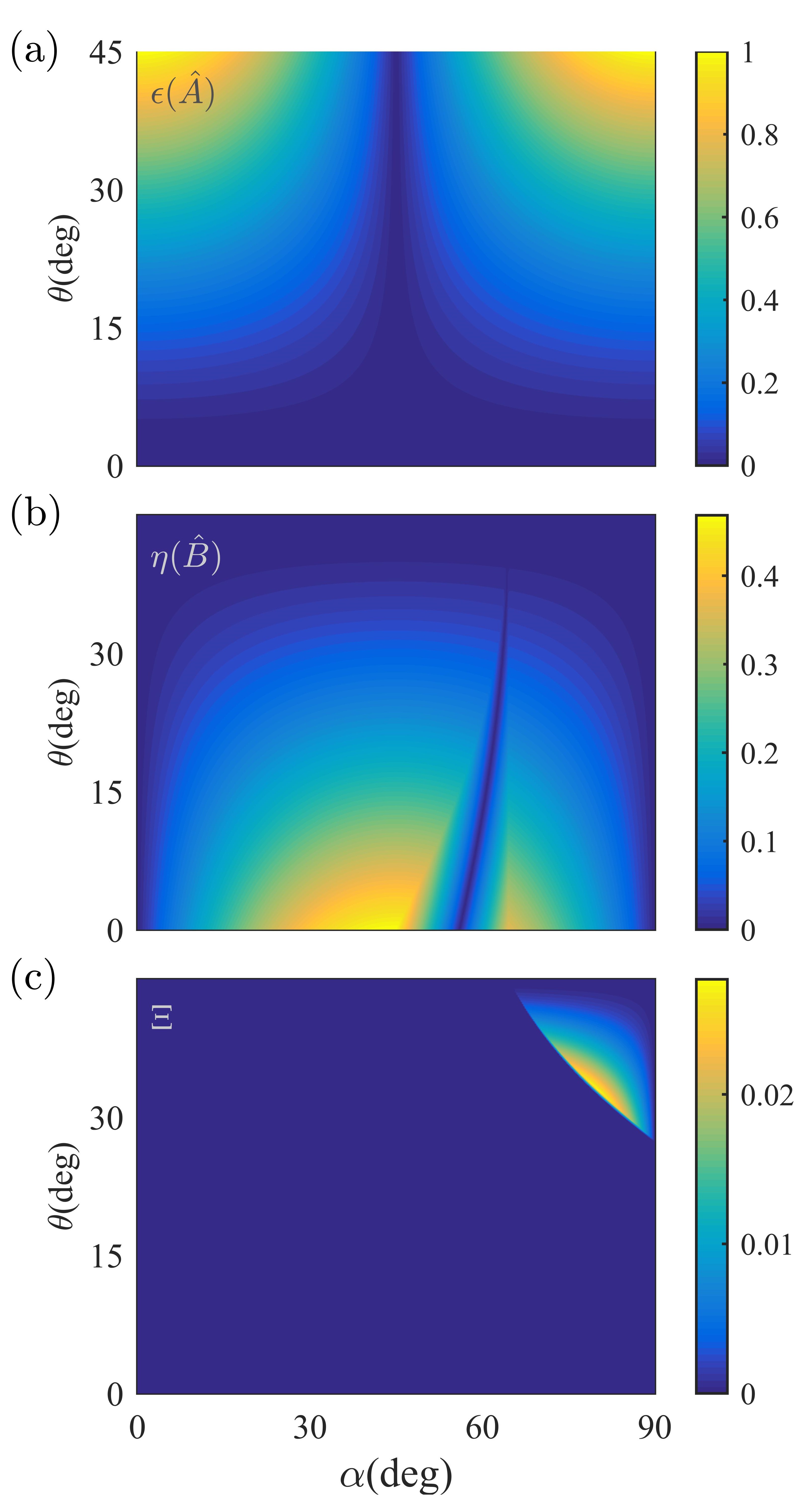 Figure 1
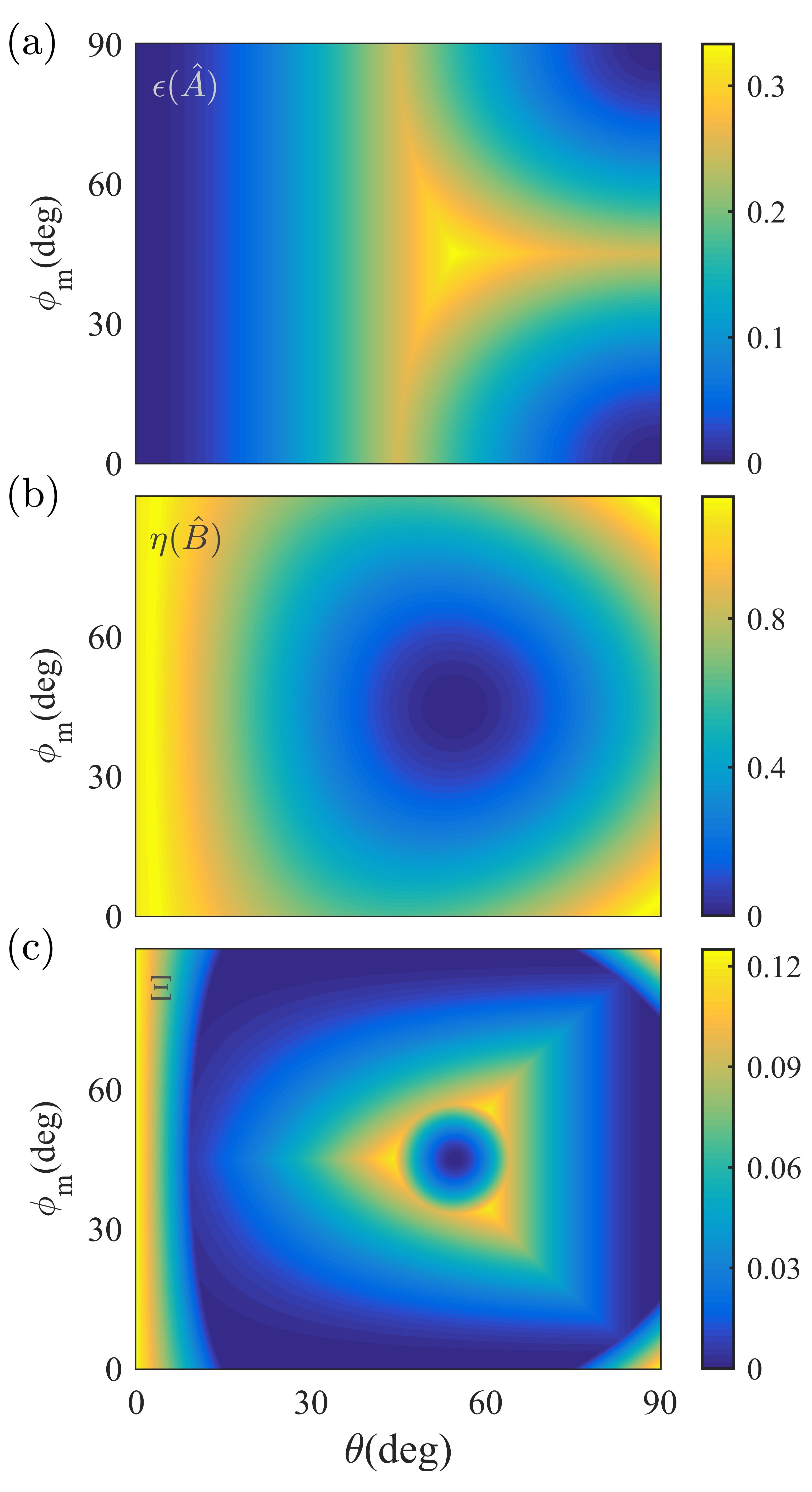 Figure 2
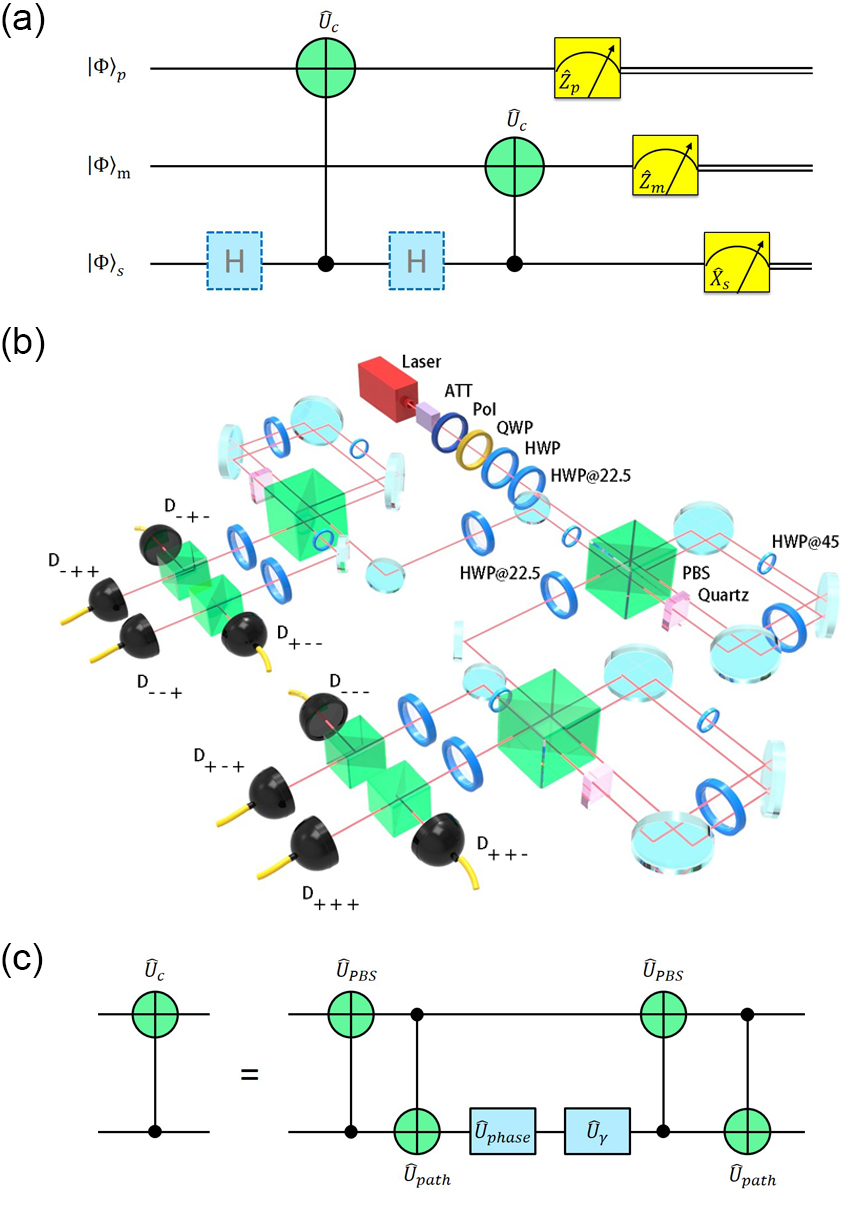 Figure 3
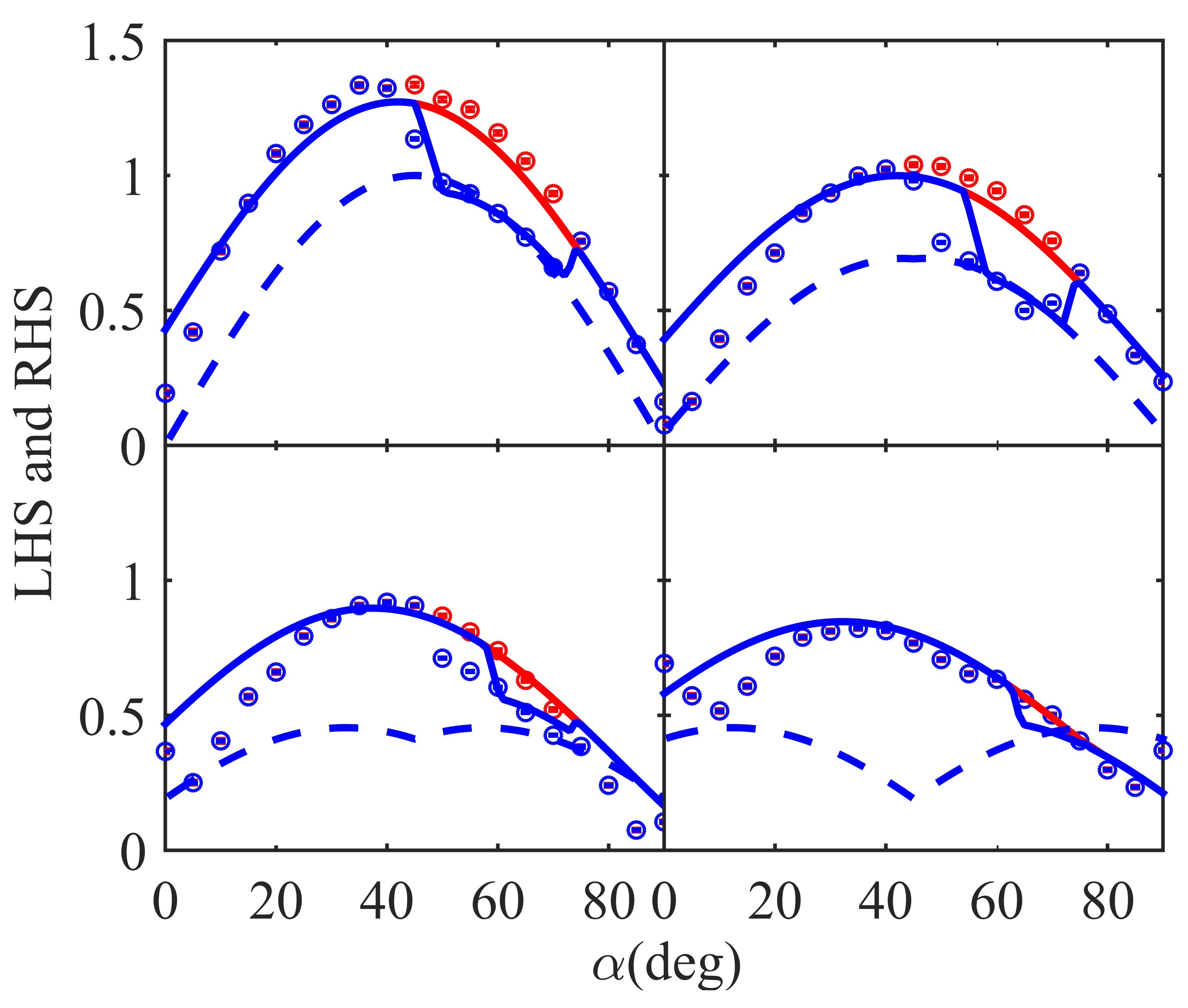 Figure 4
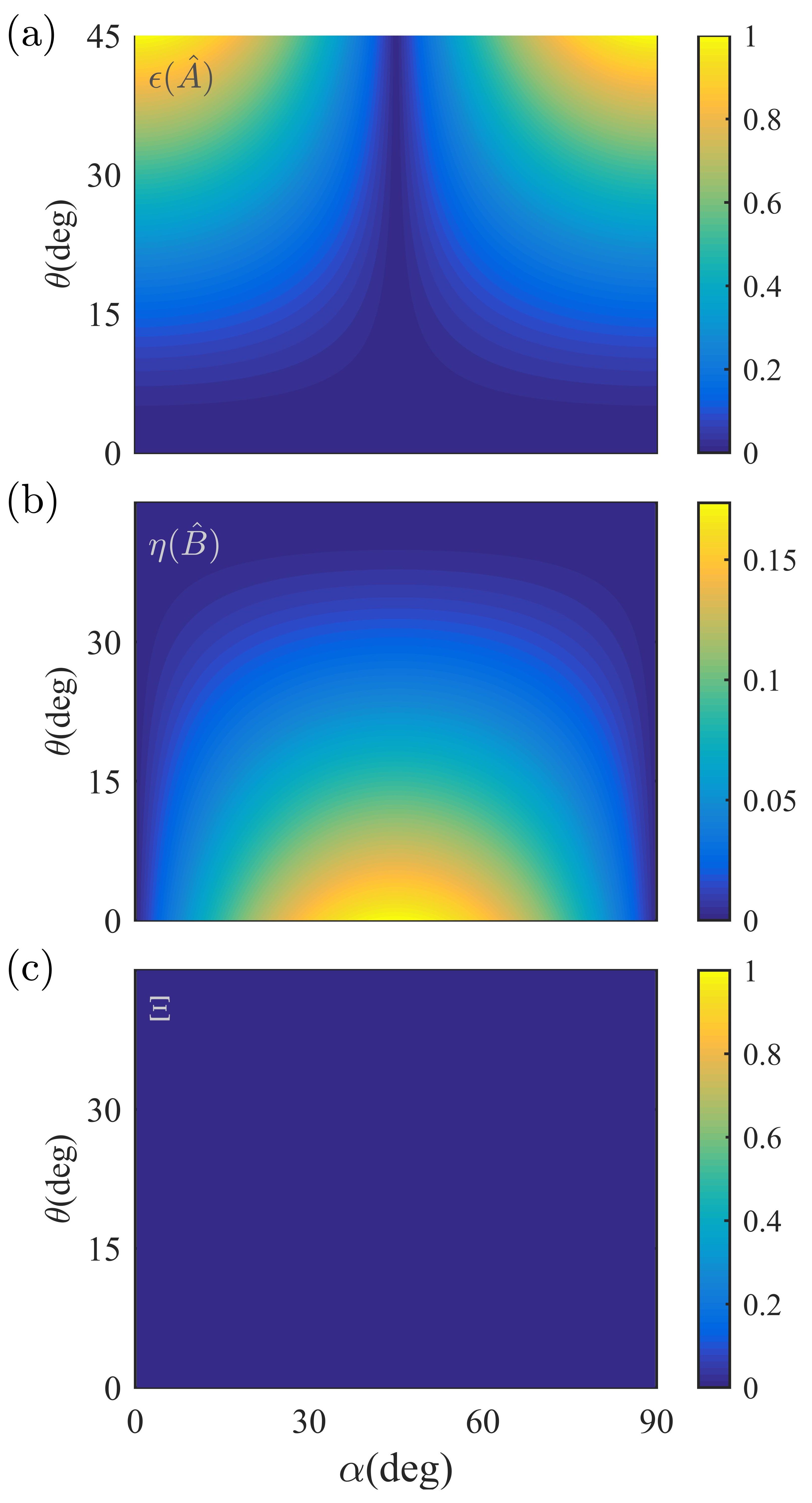 Figure 5
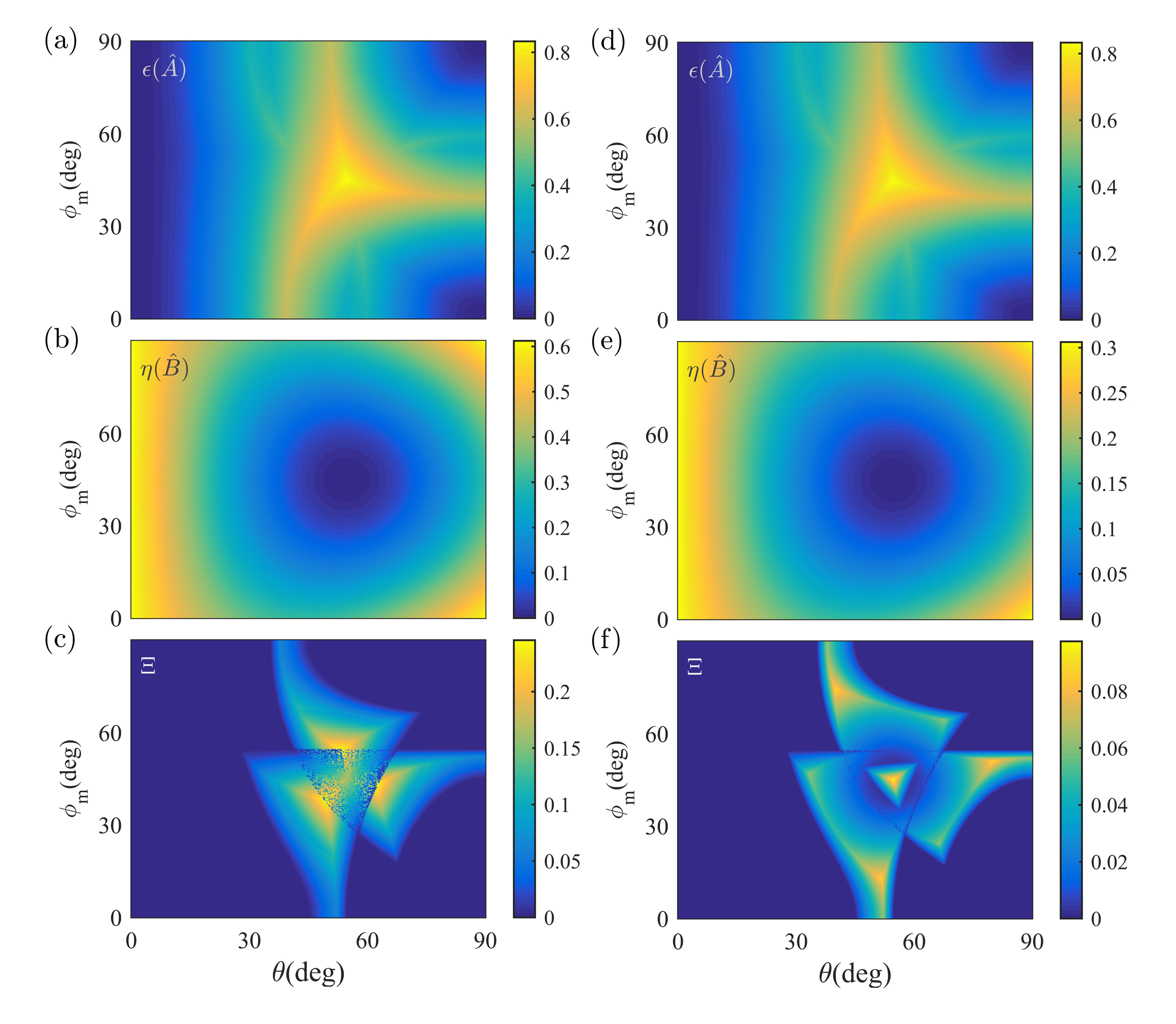 Figure 6
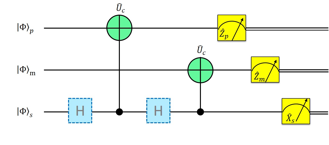 Figure 7
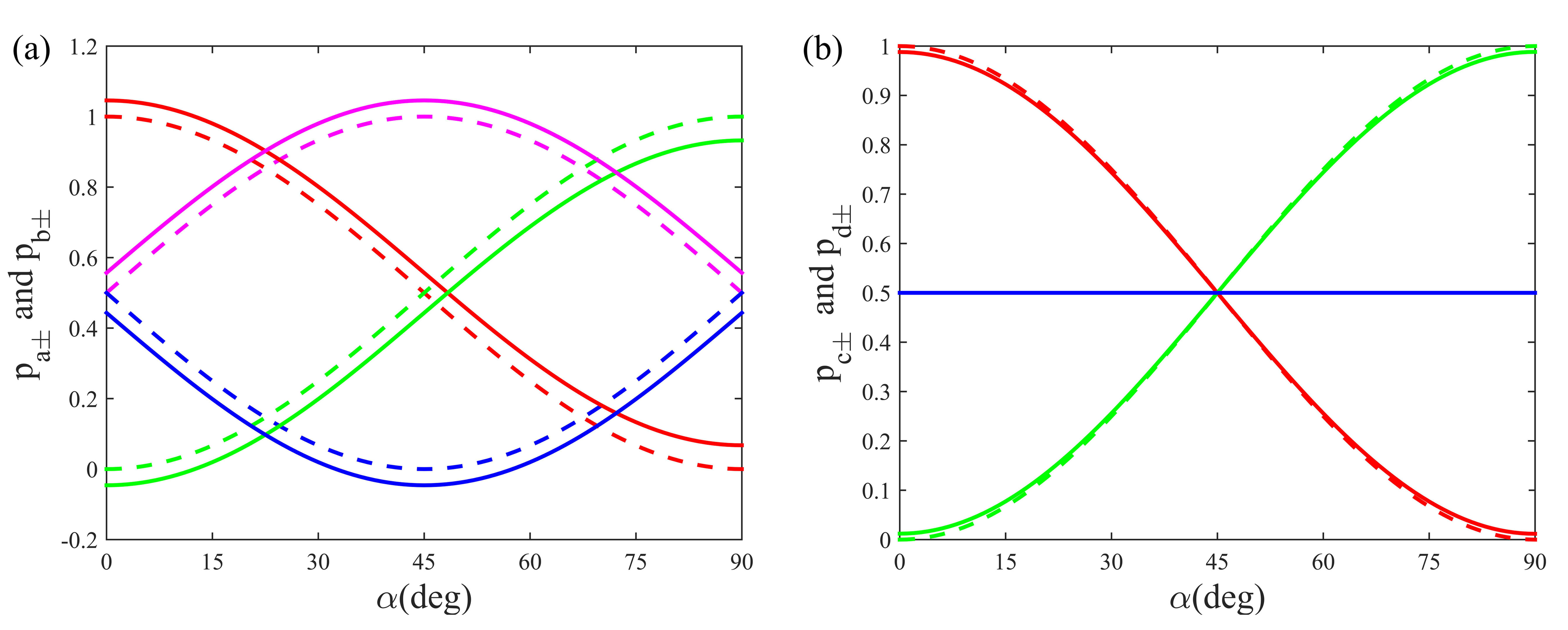 Figure 8
 Figure 9
 Figure 10
Peer Reviews
No public reviews on file for this paper yet. If you reviewed it on a platform where reviews are public (OpenReview, ICLR, NeurIPS, ICML), you can paste yours below so the community can read it here.
Videos
No videos yet. Explain this paper in a talk, walkthrough, or lecture? Add one.
Error-Disturbance Trade-off in Sequential Quantum Measurements
Ya-Li Mao
Department of Modern Physics and National Laboratory for Physical Sciences at Microscale, Shanghai Branch, University of Science and Technology of China, Hefei, Anhui 230026, China
CAS Center for Excellence and Synergetic Innovation Center in Quantum Information and Quantum Physics, Shanghai Branch, University of Science and Technology of China, Hefei, Anhui 230026, China
Zhi-Hao Ma
School of Mathematical Sciences, Shanghai Jiao Tong University, Shanghai 200240, China
Rui-Bo Jin
Hubei Key Laboratory of Optical Information and Pattern Recognition, Wuhan Institute of Technology, Wuhan 430205, China
Qi-Chao Sun
Department of Modern Physics and National Laboratory for Physical Sciences at Microscale, Shanghai Branch, University of Science and Technology of China, Hefei, Anhui 230026, China
CAS Center for Excellence and Synergetic Innovation Center in Quantum Information and Quantum Physics, Shanghai Branch, University of Science and Technology of China, Hefei, Anhui 230026, China
Shao-Ming Fei
School of Mathematical Sciences, Capital Normal University, Beijing 100048, China
Max-Planck-Institute for Mathematics in the Sciences, 04103 Leipzig, Germany
Qiang Zhang
Department of Modern Physics and National Laboratory for Physical Sciences at Microscale, Shanghai Branch, University of Science and Technology of China, Hefei, Anhui 230026, China
CAS Center for Excellence and Synergetic Innovation Center in Quantum Information and Quantum Physics, Shanghai Branch, University of Science and Technology of China, Hefei, Anhui 230026, China
Jingyun Fan
Department of Modern Physics and National Laboratory for Physical Sciences at Microscale, Shanghai Branch, University of Science and Technology of China, Hefei, Anhui 230026, China
CAS Center for Excellence and Synergetic Innovation Center in Quantum Information and Quantum Physics, Shanghai Branch, University of Science and Technology of China, Hefei, Anhui 230026, China
Jian-Wei Pan
Department of Modern Physics and National Laboratory for Physical Sciences at Microscale, Shanghai Branch, University of Science and Technology of China, Hefei, Anhui 230026, China
CAS Center for Excellence and Synergetic Innovation Center in Quantum Information and Quantum Physics, Shanghai Branch, University of Science and Technology of China, Hefei, Anhui 230026, China
Abstract
We derive a state-dependent error-disturbance trade-off based on a statistical distance in the sequential measurements of a pair of noncommutative observables and experimentally verify the relation with a photonic qubit system. We anticipate that this Letter may further stimulate the study on the quantum uncertainty principle and related applications in quantum measurements.
††preprint: APS/123-QED
Introduction.—Uncertainty is an essential feature of quantum mechanics, which underlies the quantum measurement and the emerging quantum information science Busch et al. (2014a); Coles et al. (2017) and is best reflected in the joint measurements of a pair of noncommutative observables and . When measured separately, their measurement precisions, denoted by standard deviations and , are jointly constrained by the celebrated Heisenberg-Robertson relation, Heisenberg (1927); Kennard (1927); Robertson (1929). For sequential (or joint) measurements that are an important aspect of the quantum uncertainty principle, a simple and intuitive trade-off between the error and the disturbance has remained a long-sought goal Scully et al. (1991); Storey et al. (1994); Wiseman and Harrison (1995). Heisenberg’s intuition, Heisenberg (1927), was negated in the experiments Erhart et al. (2012); Rozema et al. (2012); Baek et al. (2013); Sulyok et al. (2013, 2013); Kaneda et al. (2014); Ringbauer et al. (2014). Ozawa recently showed that the error and disturbance quantified by the root-mean-square (rms) deviations, and , satisfy the following relation Ozawa (2003, 2004a, 2004b),
[TABLE]
where and are noise operators, and the unitary operator couples the system state to the meter state . [] is extracted as the rms difference between the value of () measured with the initial system state and the value of () measured with the coupled state . and are analogs of the classical rms values. Relation (1) was soon verified in a number of experiments Erhart et al. (2012); Rozema et al. (2012); Baek et al. (2013); Sulyok et al. (2013), which thereafter has stimulated a great deal of interest in the investigation of joint measurability of two observables with fruitful outcomes Branciard (2013); Coles et al. (2017); Kaneda et al. (2014); Di Lorenzo (2013); Weston et al. (2013); Busch et al. (2013); Branciard (2014); Buscemi et al. (2014a); Busch et al. (2014b, c); Lu et al. (2014); Dressel and Nori (2014); Korzekwa et al. (2014); Ringbauer et al. (2014); Busch et al. (2014a); Sulyok et al. (2015); Busch and Stevens (2015); Demirel et al. (2016); Ma et al. (2016); Zhou et al. (2016); Sulyok and Sponar (2017); Barchielli et al. (2018).
Quantum mechanics is fundamentally probabilistic. A quantum measurement gives rise to a probability distribution associated with the eigenvalues of the measurement observable. While the rms (or a similar value comparison) approach uses the information of both values and probability distributions of observables, studying the joint measurability from the information theoretic perspective, which characterizes error and disturbance only based on probability distributions in the format of relative entropy, statistical distances, etc., has also been explored in depth Busch et al. (2013, 2014b, 2014c); Buscemi et al. (2014a); Sulyok et al. (2015); Ma et al. (2016); Zhou et al. (2016); Sulyok and Sponar (2017); Barchielli et al. (2018). Inspired by this remarkable progress, we present in this Letter a new study on the error-disturbance trade-off. By adopting the probability distance used in characterizing the incompatibility of the two measurements Busch et al. (2013, 2014c), we show that the error and disturbance trade-off relation in the sequential measurements are naturally constrained by a triangle inequality. This relation satisfies the natural and significant requirements for operational error and disturbance Korzekwa et al. (2014), is free of the shortcomings of relation (1) and is state dependent.
Main results.—Consider a given quantum state and two observables, and , where and ( and ) are the projective measurements with respect to the eigenvectors (eigenvalues) of and , respectively. The measurement () on state gives rise to the probabilities of obtaining (): []. We define the statistical distance, . The statistical distance has the following properties: and if two statistics coincide.
Similarly, we introduce as a complete set of projective measurements on the meter state, with and with as complete sets of projective measurements with respect to the noise operators and , respectively. Correspondingly, one has probabilities and . In terms of statistical distance, the error and disturbance are defined by
[TABLE]
where the minimization takes over all index permutations of .
We rewrite Eq. (2) as , and Eq. (3) as by relabelings the subindices of and , respectively. Correspondingly, we have and . Utilizing the triangle inequality for any metric functions, we have and . Therefore, we obtain . Taking into account that (similarly for ), we define , where the maximization takes over all index permutations . We then reach the following theoretical result:
Theorem 1.—The sequential measurements associated with observables and satisfy the following error-disturbance trade-off,
[TABLE]
We note that and are the general measurement operators associated with and , respectively. The lower bound may be viewed as the error induced by the general measurements. if and reduce to and for sharp measurements.
We notice that relation (1) is “nonideal” Buscemi et al. (2014a, b) at several aspects. For maximally mixed states, the right hand side (RHS) of relation (1) vanishes for any and . It is not physically reasonable that can vanish for noisy measurements, while needs not to vanish for nondisturbing measurements. Note that in Demirel et al. (2016) the right hand side of relation (1) is replaced by a stronger constant given by , which does not vanish for a maximally-mixed state. In addition, relation (1) varies with the relabelings of eigenvalues and measurement outcomes. We remark that relation (4) is free of these shortcomings. Relation (4) is also state dependent, which is different from previous state independent results from the information perspective Busch et al. (2014a, 2013, b, c); Buscemi et al. (2014a); Barchielli et al. (2018). Furthermore, we note that our statistical distance-based measures of error and disturbance satisfy the natural and significant requirements for operational error and disturbance Korzekwa et al. (2014). We present below two theoretical analyses of relation (4) for qubit and qutrit, followed by an experimental verification of relation (4) in the photonic qubit system. We note that the Wasserstein-2 distance was used in characterizing the incompatibility of the two measurements Busch et al. (2013, 2014c); Sulyok and Sponar (2017), which coincides with trace distance for the qubit case up to a constant factor 2 Busch et al. (2014c).
We plot the error and disturbance computed with Eqs. (2) and (3) for the measurements of a pair of noncommutative Pauli operators and on qubit, respectively, in Figs. 1(a) and 1(b), which generally exhibit a complementary feature between error and disturbance (see Supplemental Material Sec. I). Defining , we plot the value of in Fig. 1(c). It is evident that , hence confirming relation (4). We note that if and in their Bloch representations and are orthogonal, , we have , the complementary property is more pronounced (see Supplemental Material Sec. I). The stripe appearing on the lower part of Fig. 1(b) is due to the nonorthogonal part, which may be interpreted as the partial information gained in the measurement of that is compatible with the measurement of .
We plot the computed error and disturbance for the measurements of a pair of noncommutative angular momentum observables on qutrit, with and , , respectively in Figs. 2(a) and 2(b), which exhibits a clear complementary feature (see Supplemental Material Sec. I). We plot the value of in Fig. 2(c). It is evident that , hence confirming relation (4).
We now present an experimental verification of relation (4) with the measurements of a pair of noncommutative Pauli operators and on a photonic qubit system. The quantum circuit for the experimental implementation is given in Fig. 3(a) Lund and Wiseman (2010). The system qubit is sequentially coupled (via a unitary operation ) to a probe qubit, , and a meter qubit, . All three states are normalized. The quantum circuit yields eight joint measurement outcomes , with , and , which are completely described by a set of positive-operator-valued measures (POVMs) , with , and . Denote , and , with . Here the one-to-one correspondence is given between and , and , and and . Associated with the POVMs, the probabilities , , , and in relation (4) are given by (see Supplemental Material Sec. II),
[TABLE]
where and . It is straightforward to show that the error and disturbance trade-off relation (4) holds tight (dashed lines in Fig. 4).
Experimental implementation.—As shown in Fig. 3(b), we encode the system, probe and meter qubits using the polarization and path degrees of freedom of single photons, respectively. We first attenuate the emission of a continuous wave, distributed feedback laser with a linewidth of 2 MHz at 1560 nm to approximate a single photon source, with . We then pass the single photons through a polarizer (with polarization extinction better than ). With a pair of half and quarter wave plates, we can create arbitrarily a polarization qubit on the Bloch sphere as the system qubit, , where is the angle of the fast axis of a HWP oriented from the vertical, states and stand for horizontal and vertical polarization states and , respectively, and is the phase. The probe qubit, , is encoded with the path degree of freedom of single photons, with for clockwise and for counterclockwise propagation states in the Sagnac interferometer.
We implement the unitary coupling of the system qubit, , to the probe qubit with a Sagnac interferometer Lund and Wiseman (2010); Busch and Stevens (2015), with illustrated in Fig. 3(c). Both and are CNOT gates. While is implemented with a polarizing beam splitter (PBS) with polarization qubit as the control and the path qubit as the target, is implemented with a half wave plate oriented at (HWP@45) from the vertical with the path qubit as the control and the polarization qubit as the target. is a -phase gate, where we simply use the fact that single photons in state acquire a phase with respect to photons in state upon reflection on a mirror. describes the coupling of the polarization qubit to path qubit by a HWP.
We subsequently couple the system qubit to the meter qubit with two Sagnac interferometers to account for the two paths (see Supplemental Material Sec. III). Note that a quartz plate is used to null the phase difference between the clockwise and counterclockwise propagation states in the interferometer, and HWPs are inserted to realize the Hadamard gate for the measurement of .
We use InGaAs single photon detectors [labeled by in Fig. 3(b), with ] to detect single photons from the eight output ports in the experiment, with the gating window of the detectors set to 2 ns and the duty cycle set to 1 s to reduce background noise. With the number of single photon detection events at the eight output ports, , we compute the probabilities as , , and , respectively, where . We then obtain for the measurement of (), and .
Note that varies from for no coupling to for projective (sharp) measurement. We set to work in the weak measurement limit in the experiment.
For the linearly polarized system qubit, , we vary in the experiment the linear polarization of the system qubit from state to state and the strength to couple the system qubit to the meter qubit from zero for no coupling to one for projective measurement. As we noted earlier in the text, we have in this case. For a better illustration, we plot the values of the LHS and RHS of relation (4) (red and blue circles), respectively, in Fig. 4. They generally coincide with each other with a few exceptions that the LHS is greater than RHS. By incorporating the imperfection of PBS, i.e., the imperfect PBS reflects (transmits) a very small percentage of single photons in state (), we theoretically reproduce the experimental observations (smooth line), hence verifying the error-disturbance relation (4). (see Supplemental Material Sec. IV for details and V for results on the circularly polarized system qubit).
Conclusion.—We theoretically derived and experimentally verified that the summation of error and disturbance quantified by the statistical distance is lower bounded by a tight inequality. This new trade-off relation is free of the shortcomings of relation (1) and the lower bound is state dependent. We anticipate that our work may stimulate further investigations on quantum uncertainties and applications in measurement science.
This work has been supported by the National Key R&D Program of China (2017YFA0303900, 2017YFA0304000), National Fundamental Research Program, Chinese Academy of Sciences, National Natural Science Foundation of China (11675113) and Key Project of Beijing Municipal Commission of Education (KZ201810028042).
Y-L. M., and Z-H. M. contributed equally to this work.
Supplemental Materials: Error-Disturbance trade-off in Sequential Quantum Measurements
I The theoretical results of
According to the main text, we consider a given quantum state , meter state , and two observables, and , where and ( and ) are the projective measurements with respect to the eigenvectors (eigenvalues) of and , respectively. The measurement () on state gives rise to the probabilities of obtaining (): ().
Following the indirect measurement model Lund and Wiseman (2010), with and with are complete sets of general measurements with respect to sharp measurements and , respectively. Here we set with as a complete set of projective measurements on the meter state. In the following we examine our error-disturbance trade-off for qubits and qutrits.
I.1 The theoretical results of for qubits
We consider the system state , so the density matrix is , where and are the three Pauli matrices. The meter state is , with the density matrix and . The unitary operater is a Controlled-NOT (CNOT) gate, . We choose two observables and with and . Consequently, we have
[TABLE]
where and . Correspondingly, the measurement errors () of the observables () are given by
[TABLE]
where
[TABLE]
For , we have
[TABLE]
We then have
[TABLE]
For , we have
[TABLE]
we then have
[TABLE]
We now consider two cases:
. reduces to , and we have
[TABLE]
It is obvious that . Hence the relation (4) is tight .
We plot the error and disturbance computed for the measurements of a pair of noncommutative Pauli operators and on qubit respectively in Fig. 5(a) and (b), which generally exhibits a complementary feature between error and disturbance. We plot the value of in Fig. 5(c). It is evident that , hence confirming our relation.
. We set and , see the main text.
I.2 The theoretical results of for qutrits
We consider the sets of angular momentum operators {, , }, with . We set with eigenvalues 1, 0 and -1. The corresponding eigenvectors
[TABLE]
we then have
[TABLE]
We consider , with eigenvalues 1, 0 and -1, and eigenvectors
[TABLE]
Accordingly, we take the measurements on the meter state and the unitary operater Wilmott (2011) as:
[TABLE]
We consider a system state , where , , and . The meter state is , where . We compute , , and , which are given as
[TABLE]
Note that for and , we have , the measurement of is identical to the measurement of , which is the projective measurement performed on the meter state. For , we have , which is the weak measurement limit in this case.
For a given system state, with , , and (, ), we plot the computed error, disturbance and for the measurements of and in Fig. 6(a)–(c) (6(d)–(f)), respectively. It is evident that , hence confirming relation (4).
II Calculation of the probabilities of four measurements: , , and for qubit state
In this section, we detailedly analyze the quantum circuit model Lund and Wiseman (2010); Busch and Stevens (2015) of measuring and in Fig. 7 (Fig. 1 (a) in the main text). The top and middle wires represent the probe state and the meter state , while the bottom wire corresponds to the system state , where, for convenience, we replace and in the main text with and , respectively. Each state is in a 2-dimensional Hilbert spaces , and , respectively. It is obvious that we can prepare in Hilbert space as the input state. All three states are properly normalized. The system state is sequentially coupled to the probe qubit and the meter qubit by two CNOT gates. Two Hadamard gates are inserted to the system state before and after the first CNOT gate when the weak measurement for is taken. The projective measurement , , is separately performed on the probe state, meter state and system state, with the corresponding measurement outcomes represented by , and , respectively. Then, the outcomes of our scheme can be described as joint measurement of three three valued observables, with probabilities
[TABLE]
which are determined by a set of positive-operator-valued-measures (POVMs) . Associated with the POVMs, it is straightforward to calculate the probabilities , , and of the measurements , , , , respectively. Next, we will show the calculation of , , and in detail.
II.1 Calculation of the probabilities and for qubit state
Following the procedures in Ref Busch and Stevens (2015), after coupling the input system state to the probe state by the first CNOT gate, the state is given as
[TABLE]
where
[TABLE]
Then, the meter state is added into the whole system through the second CNOT gate. Hence the final system state is evolved to be
[TABLE]
where
[TABLE]
Denote and , which are the eigenstates of . can be rewritten as
[TABLE]
Finally, we can perform the projective measurement , and on the probe state, system state and meter state, respectively. Hence, the probabilities of each outcome can be read out as =:
[TABLE]
This gives the respective 8-outcome POVMs with positive operators on the target system:
[TABLE]
According to the definition of the POVMs, represents the initial weak measurement:
[TABLE]
We take advantage of the outcomes of the weak measurement to calculate the POVM of ,
[TABLE]
Correspondingly, the probabilities of measuring observable are given by
[TABLE]
Following the similar procedure, the POVM of , which is the general measurement associated with the observable , can be calculated,
[TABLE]
The probabilities with respect to are:
[TABLE]
II.2 Calculation of the probabilities and for qubit state
In order to get the probabilities and , two Hadamard gates are inserted to the system state before and after the first CNOT gate. Everything else in the model is entirely identical as before. We still continue to perform similar steps. Firstly, the state is given by
[TABLE]
where
[TABLE]
Secondly, the meter state is added into the whole system through the second CNOT gate. The final system state is evolved to be:
[TABLE]
where
[TABLE]
Denote and . can be written as
[TABLE]
Finally, we can carry out the projective measurement , and on the probe state, system state and meter state, respectively. Hence, the probabilities of each outcome can be read out as :
[TABLE]
The corresponds to 8 POVM on the target system:
[TABLE]
Here represents the initial weak measurement:
[TABLE]
Associated with the POVM , one has
[TABLE]
The corresponding probabilities with respect to the observable are given by
[TABLE]
Similarly, for the POVM , which is the general measurement associated with the observable , we have
[TABLE]
with the corresponding probabilities
[TABLE]
III The Sagnac interferometer
In the Sagnac interferometer in Fig. 1 (b) Kaneda et al. (2014), the polarization and path degree of freedoms of single photons acts as the system qubit and probe (meter) qubit, respectively. The polarization beams plitter (PBS) serves as the CNOT gate controlled by system qubit. The probabilities of joint measurement are strongly correlated with the performance of PBSs in the measurement setup. In order to take account of the unideal extinction ratio of PBS Baek et al. (2013), we define the reflection extinction ratio as follows:
[TABLE]
where the quantities and are the PBS reflectance of vertical polarization and horizontal polarization, respectively. It’s obvious that when , . We also define are the PBS transmittance of vertical polarization and horizontal polarization. The PBS behaviour can be accounted by the general unitary matrix:
[TABLE]
We discuss the performence of the Sagnac interferometer with the perfect and imperfect PBSs in sequence.
III.1 The Sagnac interferometer with the perfect PBSs
In the ideal case, the parameters of the PBS satisfy , , and . Hence the unitary matrix . is a CNOT gate by a half-wave plate (HWP) oriented at with path qubit as control and polarization qubit as target: . The is the -phase gate induced by the difference between the reflections of and polarized photons on mirrors. is used to couple polarization qubit and path qubit with a HWP. Then the matrix of the Sagnac interferometer can be described by
[TABLE]
We prepare the input state . After passing through the Sagnac interferometer, the output state is evolved into . By introducing the measurement operators with , the measurement can be described as
[TABLE]
where
[TABLE]
The corresponding POVM elements are
[TABLE]
For two Sagnac interferometers after the weak measurement, we replace with , with . It’s similar to obtain that . The corresponding POVMs are .
III.2 The Saganc interferometer with the imperfect PBSs
In the real experiment, all the instruments are not perfect. Therefore, it is necessary to consider the POVMs of the Sagnac interferometer with the imperfect extinction ratio of PBSs. Suppose that the extinction ratio of two sides of the PBS diagonal plane is and , the unitary operator of the quantum circuit in Fig. 2 (c) is given by
[TABLE]
where , , and . Similarly,the measurement operators are given by
[TABLE]
[TABLE]
The corresponding POVM elements are
[TABLE]
where
[TABLE]
Expressing in terms of the parameters , we have
[TABLE]
It is obvious that with the perfect PBS, there are , and . Hence the coefficients of Pauli matrices are
[TABLE]
The POVMs in Eq. (51) reduce to that of Eq. (47).
IV Analysis of the experimental results for the linearly polarized system qubit
In the section II, the probabilities of is given by in the Eq. (27), where we consider the ideal CNOT gate. For the linearly polarized system qubit, , it is obvious that the LHS and RHS of the relation (4) coincide, and they are symmetrical along the straight line in the ideal case, which is shown in the Fig. 3 of the main text. But they are no longer symmetrical in the practical experiment. There is a gap near between red and the blue dots, and the gap becomes smaller as the measured strength becomes smaller (from figure (a) to (e)). It can also be seen that the experimental results are reconstructed by the dashed line when we take the imperfect PBS into account. Therefore the imperfect PBS is the most important factor influencing the results of the experiment. Below we analyze how it affects the results in detail.
In the last section, we have discussed the Sagnac interferometer with the imperfect PBSs in the subsection B, where we calculated the POVMs in Eq. (51). If we use these POVMs to calculate the probabilities , we can find that
[TABLE]
For the linearly polarized system qubit, we have , , . Combining the coefficients and in the Eq. (52) or (LABEL:eq:CEO2), the probabilities can be simplified to
[TABLE]
where
[TABLE]
In a similar way, we can calculate the probability by adding Hardmard gate before and after the Sagnac interferometer.
[TABLE]
where and in the Eq. (56) and (LABEL:eq:pb) are the key parameters. It is obvious that the expressions in the Eq. (56) and (LABEL:eq:pb) reduce to the ideal results and , respectively, when , and .
In the following, all dashed lines are the results with the perfect PBSs, while the smooth lines are the theoretical results with corrected imperfection in PBSs, .
In the Fig. 8(a), , , and are plotted by red, green, purple, and blue lines, respectively. We note that and are greater than 1 for some input states, meanwhile the corresponding and are less than 0, due to the system imperfection in the experiment. While the impact is not so severe for the general measurements and , whose probabilities are direct physical observations. The probabilities , , and are plotted by red, green, purple, and blue lines in the Fig. 8(b), respectively, with the measurement strength . It is obvious that the and have a very slight difference in the ideal and unideal cases, they are symmetrical with respect to line . Moreover, and are always 0.5. So the main influence to the LHS and RHS are the probabilities , , and . By direct calculation we have
[TABLE]
and , see Fig. 9, where the red, cyan, black, and blue lines correspond to the results (LHS), , , (RHS). It is clear why the experimental results of LHS and RHS do not coincide for some system states.
V Experimental results for the circularly polarized system qubit
For the circularly polarized system qubit, we also set the angle in the measurement strength to , , , and , respectively. In each measurement strength, we scan the angle in the system state from to . All the experimental results of LHS (red circles) and RHS (blue circles) are shown in the Fig. 10, the former is always greater than or equal to the latter.
The reference list from the paper itself. Each links out to its DOI / PubMed record.
- 1Busch et al. (2014 a) P. Busch, P. Lahti, and R. F. Werner, Rev. Mod. Phys. 86 , 1261 (2014 a) . · doi ↗
- 2Coles et al. (2017) P. J. Coles, M. Berta, M. Tomamichel, and S. Wehner, Rev. Mod. Phys. 89 , 015002 (2017) . · doi ↗
- 3Heisenberg (1927) W. Heisenberg, Z. Phys. 43 , 172 (1927) . · doi ↗
- 4Kennard (1927) E. H. Kennard, Z. Phys. 44 , 326 (1927) . · doi ↗
- 5Robertson (1929) H. P. Robertson, Phys. Rev. 34 , 163 (1929) . · doi ↗
- 6Scully et al. (1991) M. O. Scully, B.-G. Englert, and H. Walther, Nature (London) 351 , 111 (1991) . · doi ↗
- 7Storey et al. (1994) P. Storey, S. Tan, M. Collett, and D. Walls, Nature (London) 367 , 626 (1994) . · doi ↗
- 8Wiseman and Harrison (1995) H. Wiseman and F. Harrison, Nature (London) 377 , 584 (1995) . · doi ↗