Partial invariants, large-scale dynamo action, and the inverse transfer of magnetic helicity
Nicholas Rathmann, Peter Ditlevsen

TL;DR
This paper investigates how partially conserved quantities in MHD turbulence influence inverse energy transfer and large-scale dynamo action, using spectral decomposition and shell models to analyze the role of local and nonlocal interactions.
Contribution
It identifies new enstrophy-like invariants in spectral triad interactions that help explain inverse magnetic helicity transfer and dynamo processes in MHD turbulence.
Findings
Partial invariants help understand spectral energy flux contributions.
Inverse energy transfer can occur if enstrophy-like interactions are favored.
Shell model simulations support the role of partial invariants in energy transfer mechanisms.
Abstract
The existence of partially conserved enstrophy-like quantities is conjectured to cause inverse energy transfers to develop embedded in magnetohydrodynamical (MHD) turbulence, in analogy to the influence of enstrophy in two-dimensional nonconducting turbulence. By decomposing the velocity and magnetic fields in spectral space onto helical modes, we identify subsets of three-wave (triad) interactions conserving two new enstrophy-like quantities which can be mapped to triad interactions recently identified with facilitating large-scale -type dynamo action and the inverse transfer of magnetic helicity. Due to their dependence on interaction scale locality, the invariants suggest that the inverse transfer of magnetic helicity might be facilitated by both local- and nonlocal-scale interactions, and is a process more local than the -dynamo. We test the predicted embedded…
Click any figure to enlarge with its caption.
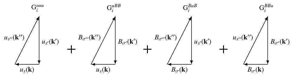 Figure 1
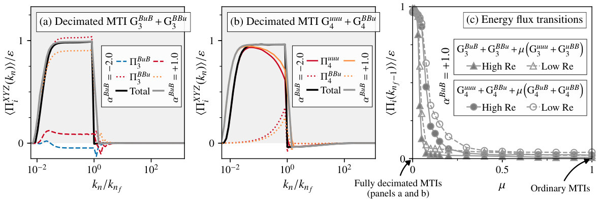 Figure 2
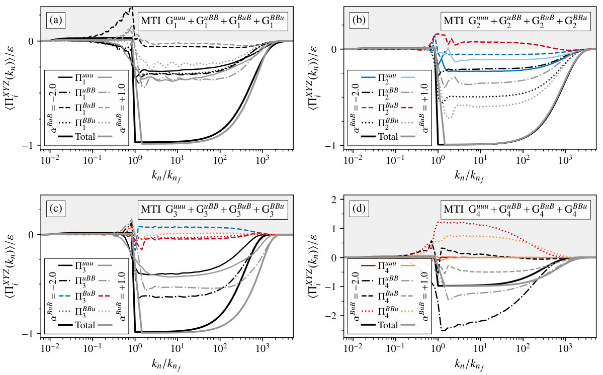 Figure 3
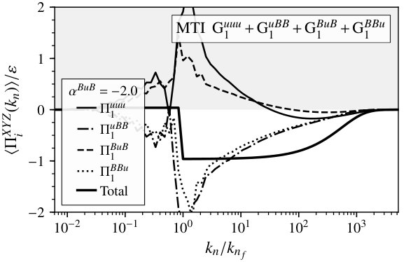 Figure 4
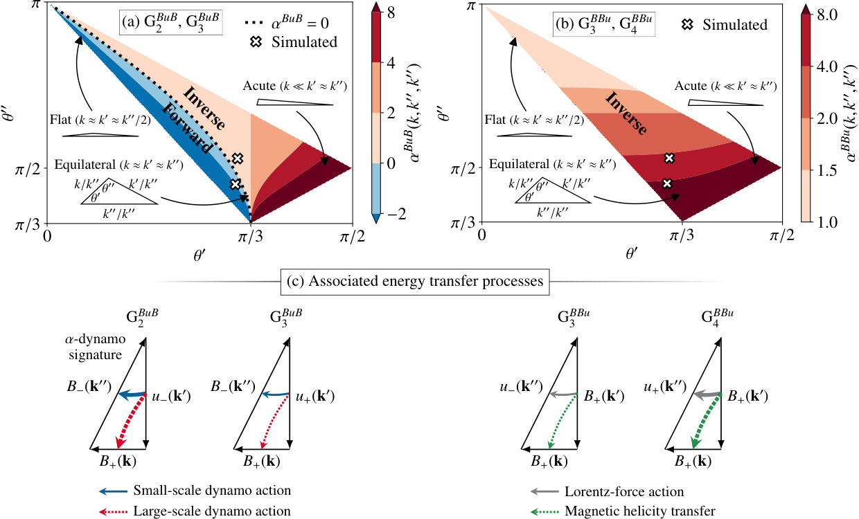 Figure 5
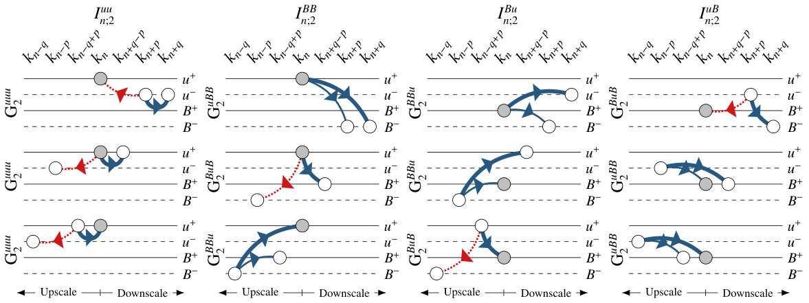 Figure 6
Peer Reviews
No public reviews on file for this paper yet. If you reviewed it on a platform where reviews are public (OpenReview, ICLR, NeurIPS, ICML), you can paste yours below so the community can read it here.
Videos
No videos yet. Explain this paper in a talk, walkthrough, or lecture? Add one.
Partial invariants, large-scale dynamo action, and the inverse transfer of magnetic helicity
Niels Bohr Institute, University of Copenhagen, Denmark
Niels Bohr Institute, University of Copenhagen, Denmark
(Received —; Revised —; Accepted —)
Abstract
The existence of partially conserved enstrophy-like quantities is conjectured to cause inverse energy transfers to develop embedded in magnetohydrodynamical (MHD) turbulence, in analogy to the influence of enstrophy in two-dimensional nonconducting turbulence. By decomposing the velocity and magnetic fields in spectral space onto helical modes, we identify subsets of three-wave (triad) interactions conserving two new enstrophy-like quantities which can be mapped to triad interactions recently identified with facilitating large-scale -type dynamo action and the inverse transfer of magnetic helicity. Due to their dependence on interaction scale locality, the invariants suggest that the inverse transfer of magnetic helicity might be facilitated by both local- and nonlocal-scale interactions, and is a process more local than the -dynamo. We test the predicted embedded (partial) energy fluxes by constructing a shell model (reduced wave-space model) of the minimal set of triad interactions (MTI) required to conserve the ideal MHD invariants. Numerically simulated MTIs demonstrate that, for a range of forcing configurations, the partial invariants are, with some exceptions, indeed useful for understanding the embedded contributions to the total spectral energy flux. Furthermore, we demonstrate that strictly inverse energy transfers may develop if enstrophy-like conserving interactions are favoured, a mechanism recently attributed to the energy cascade reversals found in nonconducting three-dimensional turbulence subject to strong rotation or confinement. The presented results have implications for the understanding of the physical mechanisms behind large-scale dynamo action and the inverse transfer of magnetic helicity, processes thought to be central to large-scale magnetic structure formation.
magnetohydrodynamics (MHD) — magnetic fields — dynamo — turbulence
††journal: ApJ
\savesymbol
tablenum \restoresymbolSIXtablenum
1 Introduction
A central problem in astrophysics is understanding how large-scale magnetic fields are generated by astrophysical bodies such as planets, stars, and galaxies (Parker, 1979). A popular explanation is that large-scale dynamo action occurs, which allows a small magnetic seed field to grow by stretching, twisting, and folding through interactions with the velocity field inside the electroconducting fluid of the body, whereby kinetic energy is converted to magnetic energy (Moffatt, 1978; Krause & Rädler, 1980; Brandenburg & Subramanian, 2005; Tobias et al., 2013). A celebrated example of a large-scale dynamo is the -effect of mean-field electrodynamics (Steenbeck et al., 1966; Moffatt, 1978; Krause & Rädler, 1980), where the mean electromotive force caused by small-scale field fluctuations is related to the large-scale magnetic field by a coefficient, . In the presence of small-scale kinetic helicity (net imbalance between left- and right-handed helical motion), the -effect leads to the development of large- and small-scale magnetic helicity of opposite signs, where the small-scale magnetic and kinetic helicity share signs (Brandenburg & Subramanian, 2005). This process can conceptually be related to a stretch-twist-fold dynamo for closed magnetic flux tubes which generates opposite signs of magnetic helicity at large and small scales (Vainshtein & Zel’Dovich, 1972; Childress & Gilbert, 1995). Combining the -effect with the influence of differential rotation (-effect), the – dynamo (Moffatt, 1978; Parker, 1979; Krause & Rädler, 1980) has widely been invoked to explain the amplification and maintenance of large-scale magnetic fields. In spiral galaxies, for example, this mechanism leads to predicted magnetic (spiral) pitch angles in the middle of observed ranges (Widrow, 2002; Brandenburg & Subramanian, 2005), among other observations in support of dynamo action (Shukurov, 2004). Likewise, large-scale solar magnetic phenomena, such as solar flares and spots, are generally attributed dynamo action in combination with differential rotation within the solar convective zone (Hood & Hughes, 2011; Brun & Browning, 2017).
Magnetic helicity is an inviscid integral of motion in magnetohydrodynamical (MHD) turbulence, and is observed in, e.g. the solar photosphere (Démoulin, 2007; Blackman, 2016) and the solar wind (Howes & Quataert, 2010), and plays a role in coronal mass ejections by effecting magnetic flux tubes topologies (Malapaka & Müller, 2013a). The inverse (upscale) transfer of magnetic helicity (Frisch et al., 1975) is another transfer process suggested to contribute to large-scale magnetic structure formation by virtue of the spectral bounds between magnetic energy and magnetic helicity (Pouquet et al., 1976; Moffatt, 1978; Biskamp, 1993). In spite of receiving a lot of attention, less is known about the nonlinear dynamics enabling an inverse transfer of magnetic helicity.
Simulations of homogeneous MHD turbulence in a box with triple periodic boundaries have been the subject of many studies attempting to better understand the conditions under which large-scale magnetic structure formation takes place due to the -effect (Brandenburg, 2001; Linkmann et al., 2017) and the inverse transfer of magnetic helicity (Alexakis et al., 2006; Müller et al., 2012; Malapaka & Müller, 2013b; Linkmann & Dallas, 2016, 2017; Linkmann et al., 2017). As an outcome, different degrees of scale locality among interactions between fields have been reported, and it is currently thought that long-range interactions might be more important in MHD turbulence than in nonconducting fluids (Mininni, 2011). On this note, we shall refrain ourselves from referring to the inverse transfer of magnetic helicity as a cascade process, since the latter is generally associated with a constant flux through wavenumber space due to scale-local interactions, which the transfer of magnetic helicity might not be (Alexakis et al., 2006; Aluie & Eyink, 2010; Müller et al., 2012).
In an attempt to better understand the mechanisms which facilitate large-scale magnetic structure formation of astrophysical interest, such as the inverse transfer of magnetic helicity and large-scale dynamo action, it is therefore important to study the nonlinear dynamics by which inviscid invariants are transferred across spatial scales. This is the focus of our work.
Role of inviscid invariants
In three-dimensional (3D), isotropic, hydrodynamical (HD) turbulence, kinetic energy is, on average, transferred from the large integral (pumping) scale of motion to the small, dissipative Kolmogorov scale (where dissipated as heat) by scale-local interactions, called a forward or direct energy cascade. In certain cases of HD turbulence, however, such as two-dimensional (2D) flows (Boffetta & Musacchio, 2010; Mininni & Pouquet, 2013) and strongly rotating 3D flows with a broken mirror symmetry (Sulem et al., 1989; Mininni et al., 2009), an inverse (or reverse) energy cascade has been observed.
In 3D HD turbulence, the dissipation of energy at the Kolmogorov scale is proportional to the enstrophy (vorticity squared) at this scale. The energy cascade in high Reynolds number turbulence must therefore be facilitated by a production of enstrophy, which is possible by means of the stretching and bending term in the vorticity equation. In 2D HD turbulence, however, the stretching and bending term is absent, and enstrophy, too, is an inviscid invariant along with energy and can only grow by increased pumping. Because the energy spectrum, , and the enstrophy spectrum, , are related by , the cascades of the two quantities cannot be treated independently, which leads to dual and counter-directional cascades whereby enstrophy cascades forwardly and energy cascades inversely (Kraichnan, 1967; Alexakis & Biferale, 2018).
In 3D HD flows, a second inviscid invariant also exists: kinetic helicity, defined as the integral of the inner product between velocity and vorticity (Moffatt, 1969; Kraichnan, 1973; Brissaud et al., 1973). In contrast to enstrophy in 2D, the effect of helicity on the directionality of the energy cascade in 3D is less understood. Although the helicity spectrum can also dominate over the energy spectrum at small scales (large wavenumber, ) as enstrophy, helicity is not sign definite as opposed to enstrophy. As a consequence, helicity does not place similar restrictions on the direction of the energy cascade (Alexakis & Biferale, 2018).
By decomposing the velocity field in spectral space onto helical modes, each velocity component evolves according to the Navier–Stokes equation by helical three-wave (triad) interactions which separately conserve kinetic energy and kinetic helicity (Constantin & Majda, 1988; Waleffe, 1992). Recently, new additional quantities were identified that are partially conserved among helical triad interactions (De Pietro et al., 2015; Rathmann & Ditlevsen, 2016, 2017), henceforth referred to as pseudo-invariants or partial invariants; that is, quantities which are conserved only by a subset of all possible helical triad interactions.
In a further subset of helical triad interactions, the associated pseudo-invariants become enstrophy-like and have been suggested to induce embedded (partial) inverse energy cascades in 3D HD turbulence (Rathmann & Ditlevsen, 2017) [relevant to the interpretation of other numerical studies such as Biferale et al. (2012); De Pietro et al. (2015); Alexakis (2017); Sahoo et al. (2017a)]. Since these triad interactions are predominantly responsible for channelling energy upscale within rotating flows (Buzzicotti et al., 2018), and with possible relevance for thin-layered turbulence (Benavides & Alexakis, 2017), there are reasons to believe that inverse energy transfers might generally exist embedded in 3D HD turbulence due to partial invariants with implications for the net transfer of energy.
Because of their clear physical interpretation, quadratic invariants, such as enstrophy, play a central role in the study of turbulent cascade dynamics. In this work, we conjecture that the spectral–helically decomposed energy fluxes in ideal MHD turbulence might also be understood in terms of pseudo-invariants, which has potential implications for large-scale magnetic structure formation insofar as the aggregate of triads interactions conserving them are relevant for the velocity and magnetic field evolutions. We show that two new enstrophy-like quantities are partially conserved by the ideal MHD equations, and argue that embedded, inverse energy transfers might develop as a result. Intriguingly, the new quantities are conserved by triad interactions recently argued to facilitate large-scale -type dynamo action and the inverse transfer of magnetic helicity (Linkmann et al., 2016). By constructing a shell model (reduced wave-space model), we show the new pseudo-invariants are indeed useful for understanding the simulated partial (forward and inverse) spectral energy fluxes and, moreover, demonstrate that strictly inverse energy transfers might develop if enstrophy-like conserving interactions are favoured, such as results for nonconducting turbulence subject to strong rotation (Buzzicotti et al., 2018) or confinement (Benavides & Alexakis, 2017) suggest.
2 The spectral–helical decomposition
In real space, the incompressible, ideal MHD equations are
[TABLE]
where is the velocity field, the magnetic field in Alfvén units, is the kinematic viscosity, the magnetic resistivity, the pressure, and the density set to for convenience. In spectral space, the divergence-free constraints on and translate into and . The helical basis (Constantin & Majda, 1988; Waleffe, 1992) exploits this property by decomposing each complex spectral component into two helical modes, , which are mutually perpendicular to and are eigenmodes of the curl operator, i.e. where . In this basis, the velocity and magnetic components are given by
[TABLE]
and the ideal MHD invariants energy (), magnetic helicity (), and cross helicity (), are given by
[TABLE]
where is a helical sign coefficient, and , , and , are the respective spectra.
Lessinnes et al. (2009) first proposed applying the decomposition also to the MHD equations (1), giving
[TABLE]
where are helical sign coefficients of the interacting helical modes, and
[TABLE]
is an interaction coefficient. Velocity modes thus evolve by helical triad (three-wave) interactions involving and , while magnetic modes evolve by helical triad interactions involving and , provided that triads close ().
Note that the splitting of the curl of the electromotive force in the induction equation into an advective term, , and dynamo (stretching) term, , is obfuscated by the spectral–helical decomposition and these terms are therefore not directly associated with the two sums in (6).
For each of the four types of helical triad interactions, distinct combinations of helical signs are possible as indicated by the sums over helical signs in (5)–(6). If sorted against shared interaction coefficients, however, only four unique sign combinations remain per triad type: for each of the triad types , , , and , the associated helical signs , , , and , respectively, may be any one of the combinations , and . From here on, these four possible combinations of helical signs shall be referred to as sign groups , respectively. Any particular helical triad interaction may therefore be referred to by a combination of the triad type and its sign group number, henceforth denoted compactly by . In this notation, refers to the sign group number, and and are placeholders for the fields of the interacting modes. Note that only the four types exist, and that is the field associated with wave-vector , with , and with .
Isolating terms in (5)–(6) involving a single triad of waves, , only four triad interactions remain per possible combination of helical signs, namely , hereafter referred to as a minimal set of triad interactions (MTI) following Linkmann et al. (2017) (Figure 1). Note that distinct MTIs are possible, and that only in the case of homochiral MTIs (, , and ) do the four MTI components share sign group numbers ().
By noting the cyclic property of , the evolution of velocity and magnetic modes in a given MTI is governed by (Linkmann et al., 2016)
[TABLE]
where the compact notations , , and are used (and likewise for ). While the relative magnitudes of energy, magnetic helicity, and cross-helicity fluxes between the three triad legs are fixed and determined by the coefficients in (7), the magnitudes and directions of the average fluxes (to or from a leg) depend on the unknown triple-correlators , and .
From this simpler form of the spectral dynamics, it follows that each MTI conserves energy, magnetic helicity, and cross-helicity, by noting
[TABLE]
The ideal MHD invariants (2)–(4) are thus conserved per triad of waves, but only collectively by the four components constituting a MTI (for any choice of helical signs), hence the notion of a minimal set.
Linkmann et al. (2016) recently proposed the behaviour of a given MTI might be understood from the linear stability of (7) around trivial steady-states, inspired by a similar approach in HD turbulence (Waleffe, 1992). Waleffe (1992) suggested that energy, on average, flows from the most unstable triad mode (leg) and in to the other two. In this regard, the behaviour of a given triad may be classified as either forward (F-class) if the smallest wavenumber mode (largest scale) is linearly unstable, suggesting that energy is transferred to the two smaller scales (forward cascade), or reverse (R-class) if either the middle or largest wavenumber modes are unstable, suggesting that energy is transferred either partly or fully to larger scales (inverse cascade), respectively. By considering the linear stability of the states , where and are constants, Linkmann et al. (2016) showed that the modes evolve by [and similarly for , but with different ]. The modal (leg) stabilities therefore depend on the existence eigenvalues for with real, positive parts, which have complicated dependencies compared to the HD case: in addition to depending on the helical signs of the three interacting modes, such as a stability analysis of the pure HD case also does, it moreover depends on the ratio , and the alignment between velocity and magnetic modes (cross-helicity).
3 The pseudo-invariants
In HD turbulence, quadratic invariants play a fundamental role in the understanding of turbulent cascade dynamics, such the energy cascade reversal in 2D which may be understood by both energy and enstrophy being strictly positive quantities and enstrophy dominating the small scales (Alexakis & Biferale, 2018). The fact that interactions in 3D conserve both signs of kinetic helicity separately is an intriguing possible explantation for the identified R-class nature of interactions (Biferale et al., 2012) in analogy to enstrophy-conserving interactions in 2D. Recently, the mixed forward–inverse behaviour exhibited by interactions depending on triad geometry (Waleffe, 1992; De Pietro et al., 2015; Rathmann & Ditlevsen, 2017) was also proposed to be explained by the existence of a new enstrophy-like pseudo-invariant , where depends on the specific triad shape and hence interaction locality in wave space (Rathmann & Ditlevsen, 2017).
Following Rathmann & Ditlevsen (2017), we here show that a subset of MHD triad interactions exists that also conserve enstrophy-like quantities, which might help in understanding the behaviour of MTIs in terms of conserved quantities in analogy to enstrophy-conserving interactions in 2D HD turbulence. Inspired by the HD pseudo-invariant, consider therefore the generalized spectral energy density defined as
[TABLE]
This quantity is thus enstrophy-like for exponents , and might induce an inverse (upscale) contribution to the total transfer of energy if conserved by triad interactions. Note that corresponds to energy which is conserved by any MTI.
Applying (7) to (8), it follows that the pseudo-invariant is conserved if , implying
[TABLE]
where [suppressing dependences on wavenumbers and helical signs in the definitions of ]
[TABLE]
Conservation by an MTI thus requires the existence of solutions that simultaneously fulfil for all . Since this is not possible, we are here interested in the possibility that the four individual MTI components (Figure 1) might separately conserve different pseudo-invariants, leading to inverse partial fluxes developing.
Equations (9)–(12) are functions of the wavenumber ratios and , and consist of a constant term and two monotonically increasing or decreasing terms.
For solutions to exist besides energy (), the signs of the three terms in each of (9)–(12) must alternate (considering the ordering without loss of generality). On inspection, it follows that only interactions solve for .
The HD pseudo-invariant associated with triads has previously been investigated (Rathmann & Ditlevsen, 2017), finding a cascade reversal indeed takes place for a nonlocal subset of triad geometries due to the invariant becoming enstrophy-like (). The pseudo-invariant associated with the velocity–magnetic triads , and have, however, not previously been considered. Unlike the HD -term (9), the -terms (10)–(12) do not depend on the helical signs of all three triad legs: the helical sign of the velocity mode does not enter (10)–(12), implying and share -terms, and thus pseudo-invariants, as do and .
Figures 2a and 2b show the numerical solutions w.r.t. for and , respectively, hereafter referred to as and . The solutions are shown for all possible (noncongruent) triad geometries (coloured area) by expressing each triad in terms of the two interior angles and using the Sine rule: and . Figure 2a shows that and interactions may, similarly to , contribute either to a forward transfer of energy (, blue colors) or inversely (, red colors). The exact transition line through the space of triad geometries separating the two behaviours is given by , yielding
[TABLE]
which corresponds to the geometries for which the energy and pseudo-invariant solutions collapse (Figure 2a, black dotted line). Figure 2b, on the other hand, shows that and interactions always conserve an enstrophy-like quantity () regardless of triad geometry, suggesting they should contribute with an inverse transfer of energy.
We have thus arrived at several testable predictions for the contributions to the total transfer of energy from the four individual MTI components: (i) triads contribute to a forward transfer (for all sign groups ), (ii) and contribute to a forward transfer while and may contribute either to a forward or inverse transfer depending on triad geometry, and (iii) and contribute to a forward transfer while and contribute inversely.
4 The MTI shell model
To test the predictions based on the pseudo-invariants, we constructed an MTI shell model (reduced wave-space model). Shell models have previously provided valuable insight into the spectral dynamics of MHD turbulence (Lessinnes et al., 2009; Plunian et al., 2013), and are especially convenient in MHD turbulence due to the added number of nonlinear interactions (Figure 1) making direct numerical simulations computationally expensive. Only relatively recently have direct numerical simulations of (5)–(6) been conducted giving some insight into the behaviour of helical MHD triad dynamics and the role of the ideal MHD invariants in the spectral–helical basis (Linkmann et al., 2017) (see section 6).
Shell models allow simulating very long inertial–inductive ranges at the expense of severely truncating spectral space: only wavenumbers distributed exponentially according to are retained, where are the shell indices, , and . The golden ratio is the upper limit such that any set of nearest neighbour waves fulfils the triangle inequality as required by (5)–(6). All spectral components are generally reduced to depend only on wave magnitudes expect for a few cases (Gürcan, 2017; Monthus, 2018; Gürcan, 2018), and shell models may therefore be regarded as simple, structureless cascade models.
The pioneering work on constructing helical shell models was done by Benzi et al. (1996), which has since inspired other helical shell models and led to important insights on helically decomposed triad dynamics of HD turbulence (Ditlevsen & Giuliani, 2001a, b; Lessinnes et al., 2011; De Pietro et al., 2015; Rathmann & Ditlevsen, 2016; Sahoo et al., 2017b; De Pietro et al., 2017) and MHD turbulence (Lessinnes et al., 2009; Plunian et al., 2013; Stepanov et al., 2015). Following Rathmann & Ditlevsen (2016) for the Navier–Stokes equations, (5)–(6) may similarly be cast into a shell model by noting that the triadic interaction structure is similar but with different interaction coefficients. Considering only homochiral MTIs (elaborated on below) with fixed shape triads (fixed interior angles) and adopting the usual shorthand notation and , the shell model for a single kind of MTI is given by
[TABLE]
where the resolved triad interactions are collected in , defined as
[TABLE]
Here, the helical signs of each sign group are for convenience referred to by , such that for groups , respectively, and the interactions coefficients are given by
[TABLE]
The integers can be related to any triangular shape through the Sine rule. The possible resolved triad shapes depend therefore on the combination of : For any triad geometry may be constructed for large/small enough values of , while for triads collapse to a line. Hence, for each chosen set of , the shell model consists, independently of scale , only of fixed-shaped triad interactions. The outer sums over all triad shapes in (5)–(6) are thus reduced to just three (fixed-shape) helical triad interactions per MTI component per resolved scale , exemplified in Figure 3 for the case of . Note that only contains triad interactions of one MTI component exclusively, namely . The remaining three (, and ) contain a mix of the velocity–magnetic triads and .
The dissipation terms are defined as and where the drag terms, and , are added the usual way to remove energy building up at large scales.
Like the ideal MHD equations (5)–(6), the MTI shell model also inviscidly conserves energy (), magnetic helicity (), and cross-helicity (), which can be shown by applying (14)–(15) to (2)–(4), telescoping sums, and inserting the boundary conditions for and . Unlike the ideal MHD equations (5)–(6), however, the MTI shell model (14)–(15) conserves all MHD invariants only if the resolved MTIs are homochiral; that is, each MTI component must share the same sign group, . Hence, the four possible shell model MTIs are for .
4.1 Forcing mechanism
The velocity () and magnetic () forcing terms may be constructed to allow full control over the pumping of energy (), kinetic helicity (), magnetic helicity (), and cross-helicity (), where the superscripts and refer to the injection fields. For the kinetic forcing term, this amounts to solving the forcing balance equations , , , and . For the magnetic forcing term, the balance equations are similar but with and interchanged, and with the balance of magnetic helicity being given by . Solving these closed sets of equations, the mechanical–electromagnetic helical forcing becomes
[TABLE]
which provides a constant pumping of energy, kinetic helicity, magnetic helicity, and cross-helicity, for constant , , , and , respectively, thus allowing the simulated spectral fluxes to easily be normalized against pumping rates.
4.2 Spectral energy flux
The total spectral flux of energy (kinetic+magnetic), carried by a homochiral MTI of sign group through the th scale, is given by , where includes only the nonlinear terms in (14)–(15). Decomposing the total flux into the four separate MTI-component contributions, or partial fluxes, such that
[TABLE]
requires isolating the terms in (14)–(15) corresponding to triad interactions , and , which can be shown to give
[TABLE]
Using these MTI-decomposed equations, the partial fluxes follow as (telescoping sums and applying the boundary conditions for and ):
[TABLE]
where the triple correlators, , are defined as
[TABLE]
5 Numerical results
For each of the four homochiral MTIs, two different triad shapes (crosses in Figure 2) were considered in order to test the partial flux predictions. The model was configured using a shell spacing of with and , corresponding to pseudo-invariant exponents of and , respectively. The chosen triad geometries thus sample contributions from both the forward and inverse parts of interaction space (Figure 2a).
For simplicity, all model simulations were configured with identical free parameters (the values of which were found not to influence results): 1\text{\times}{10}^{-8}\text{,} (i.e. a magnetic Prandtl number of one), $\nu_{L}=\mu_{L}=$1\text{\times}{10}^{1}\text{\,}, , and . The modes and were initialized in a K41-scaling state (the shell model equivalent of ) with zero helicity of any kind, and stepped forward using a fourth-order Runge–Kutta integration scheme with a time-step of 5\text{\times}{10}^{-7}\text{,}$$. The injection rates , and (i.e. no forcing handedness, elaborated on in the discussion) were evenly applied over shells, starting from shell . Thus, in the configuration, shells #31 and #32 were also forced. Note that while dynamo studies typically inject only kinetic energy, both kinetic and magnetic energy were injected in the present simulations. Although no difference in the energy flux partitioning between MTI components was found for homochiral MTIs , the magnetic field collapsed for unless magnetic energy was injected.
The simulated partial energy fluxes within the four homochiral configurations are shown in figures 4a, 4b, 4c, and 4d, respectively, calculated using (16)–(19). The energy flux partitionings are shown for both triad shapes, labeled in the legends by the corresponding exponents. Gray/black lines represent components without pseudo-invariants, whereas components marked by coloured lines posses pseudo-invariants: blue colors indicate components for which the pseudo-invariant exponents are negative (, hypothesised forward contribution), whereas red/orange colors mark components conserving enstrophy-like quantities with positive exponents (, hypothesised inverse contribution).
Figures 4a and 4b show the partitionings within homochiral MTIs and conform with the pseudo-invariant predictions: all MTI components contribute to a forward transfer, whereas (conserving an enstrophy-like quantity, ) contributes to an inverse transfer.
Figure 4c shows the partitioning within MTI almost behaving as expected: all components contribute to a forward transfer of energy, except for and interactions which have their behaviours reversed — i.e. components conserving enstrophy-like quantities are found to contribute to a forward energy transfer and vice-versa.
Figure 4d shows the partitioning within MTI also conforms with predictions: all components contribute to a forward transfer of energy, whereas (conserving an enstrophy-like quantity, ) contributes inversely. For the simulated triad shape corresponding to , however, the component carries a small inverse contribution in spite of not conserving any enstrophy-like quantity.
6 Discussion
6.1 Effect of coupling MTI components
The homochiral MTIs of sign groups and show discrepancies between simulated partial fluxes and predictions based on the pseudo-invariants (section 5).
In the case of the shell model, we find that coupling-induced effects, caused by the coupling of MTI components, might play an important role by altering the component-wise behaviours (partial fluxes) compared to predictions. This is exemplified by considering additional decimated simulations in which only and are coupled, i.e. decomposing the MTIs by disregarding and interactions. Using the same model configuration as above, Figure 5a shows the resulting energy flux partitioning between the two components and in the decimated MTI . For all four decimated MTIs (), the component-wise partial fluxes are found to conform with the pseudo-invariant predictions ( not shown), suggesting the discrepancies between the full and decimated MTIs might be due to coupling-induced effects. Whether this is a model artefact or a property also shared by large triad networks (5)–(6) is not clear.
6.2 Universality of energy flux partitioning
The partitioning of the energy cascade between symmetrized helical triad interactions was recently investigated by Alexakis (2017) in a direct numerical simulation of the spectral–helical Navier–Stokes equation. Like here, it was found that the energy cascade partitions itself into approximately constant partial-flux components within the inertial range, an intriguing result given that only the total energy flux is required to be constant. Moreover, Alexakis (2017) found that the partitioning was unaffected by the pumping of kinetic helicity, suggesting the partitioning might be universal (among a given set of resolved triads). If so, the physical explanation for the directionalities of the partial fluxes in terms of pseudo-invariants might be applicable in a general, forcing-independent sense.
Inspired by this result, we conducted additional simulations where the four homochiral MTIs were forced with kinetic helicity (), magnetic helicity (), and cross-helicity () besides energy, in contrast to the nonhelical forcing used above (). While the partitionings were found to be independent of and , suggesting the partitionings might be universal, the same was not found for a nonzero injection of cross-helicity (). This is exemplified in Figure 6 for the homochiral MTI (similar results were found for ), demonstrating the divergent, non-constant partial fluxes which develop in the case of . In addition, when pumping cross-helicity, the simulated directionalities of the partial fluxes generally do not agree with the pseudo-invariant predictions: in Figure 6, all components are predicted to contribute to a forward energy transfer since no enstrophy-like quantities are conserved.
Because the evolution of magnetic modes depends on the alignment between velocity and magnetic modes (cross-helicity) according to (6), it is not entirely surprising that injecting cross-helicity can affect the detailed partitioning. Note that this result is in agreement with a linear stability analysis which also predicts that triad leg (modal) stabilities depend on velocity–magnetic alignments (Linkmann et al., 2016).
The present analysis considered only a magnetic Prandtl number of one. While investigating large and small magnetic Prandtl number flows is out of scope of the present work, studies such as Verma & Kumar (2016) indicate that under some forcing conditions the partitioning might be unaffected, although helically decomposed dynamics were not considered in that case.
7 Conclusion
In conclusion, we identified new, partially conserved quantities among the elementary three-wave (triad) interactions in spectral–helically decomposed ideal magnetohydrodynamical (MHD) turbulence. Because the new quantities conserved by a subset of triad interactions are enstrophy-like, we conjecture that such interactions might contribute to embedded, inverse energy transfers developing in three-dimensional MHD turbulence in analogy to enstrophy-conserving triad interactions in two-dimensional hydrodynamical (HD) turbulence.
In order to test the predictions based on the new pseudo-invariants, we introduced a helically decomposed reduced wave-space model (shell model). By conducting numerical simulations of the four kinds of homochiral minimal sets of triad interactions (MTIs) (minimal in the sense of being required to conserve the ideal MHD invariants), we demonstrated the usefulness of the partial invariants for understanding the resulting embedded energy flux contributions (partial fluxes) from the triadic components constituting an MTI.
While for simplicity this study concerned itself with the case of a magnetic Prandtl number of one, we find that the embedded partial fluxes are generally constant over inertial–inductive ranges, indicating that forward and inverse energy cascades might generally exist embedded in MHD turbulence. Importantly, however, we note that the injection of cross-helicity by the forcing mechanism, and the effect of coupling certain types of MTI components (triad interactions), demonstrate cases where the directions of the simulated partial fluxes do not agree with the pseudo-invariant predictions. Whether this is a model artefact or a property shared by more comprehensive (and thus more realistic) large triad networks as represented by the spectral–helically decomposed MHD equations (5)–(6), is not clear.
The reference list from the paper itself. Each links out to its DOI / PubMed record.
- 1Alexakis (2011) Alexakis, A. 2011, Physical Review E, 84, 056330
- 2Alexakis (2017) —. 2017, Journal of Fluid Mechanics, 812, 752
- 3Alexakis & Biferale (2018) Alexakis, A., & Biferale, L. 2018, Physics Reports
- 4Alexakis et al. (2005 a) Alexakis, A., Mininni, P., & Pouquet, A. 2005 a, Physical review letters, 95, 264503
- 5Alexakis et al. (2005 b) Alexakis, A., Mininni, P. D., & Pouquet, A. 2005 b, Physical Review E, 72, 046301
- 6Alexakis et al. (2006) —. 2006, The Astrophysical Journal, 640, 335
- 7Aluie (2017) Aluie, H. 2017, New Journal of Physics, 19, 025008
- 8Aluie & Eyink (2009) Aluie, H., & Eyink, G. L. 2009, Physics of Fluids, 21, 115108