
TL;DR
This paper explores the structure and metrics of the real Jacobi group, providing explicit calculations of invariant forms, metrics, and their relations to the Siegel-Jacobi upper half-plane, enriching the geometric understanding of this mathematical object.
Contribution
It offers explicit formulas for invariant forms and metrics on the real Jacobi group and related manifolds, connecting group theory with geometric structures.
Findings
Computed left-invariant one-forms and vector fields for the real Jacobi group.
Derived invariant metrics depending on multiple parameters on associated manifolds.
Expressed the Kähler balanced metric as a sum of squares of invariant forms.
Abstract
The real Jacobi group , defined as the semi-direct product of the group with the Heisenberg group , is embedded in a matrix realisation of the group . The left-invariant one-forms on and their dual orthogonal left-invariant vector fields are calculated in the S-coordinates , and a left-invariant metric depending of 4 parameters is obtained. An invariant metric depending of in the variables on the Sasaki manifold is presented. The well known Kähler balanced metric in the variables of the four-dimensional Siegel-Jacobi upper half-plane depending…
Click any figure to enlarge with its caption.
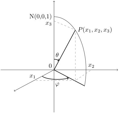 Figure 1
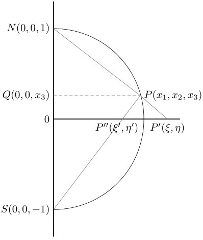 Figure 2
| Nr. cr. | a | b | c | d | e | f |
|---|---|---|---|---|---|---|
| 1 | ||||||
| 2 | ||||||
| 3 | ||||||
| 4 | ||||||
| 5 |
Peer Reviews
No public reviews on file for this paper yet. If you reviewed it on a platform where reviews are public (OpenReview, ICLR, NeurIPS, ICML), you can paste yours below so the community can read it here.
Videos
No videos yet. Explain this paper in a talk, walkthrough, or lecture? Add one.
\FirstPageHeading
\ShortArticleName
The Real Jacobi Group Revisited
\ArticleName
The Real Jacobi Group Revisited
\Author
Stefan BERCEANU
\AuthorNameForHeading
S. Berceanu
\Address
National Institute for Physics and Nuclear Engineering, Department of Theoretical Physics,
PO BOX MG-6, Bucharest-Magurele, Romania
[email protected] \URLaddresshttp://www.theory.nipne.ro/index.php/mcp-home
\ArticleDates
Received May 09, 2019, in final form November 25, 2019; Published online December 07, 2019
\Abstract
The real Jacobi group , defined as the semi-direct product of the group with the Heisenberg group , is embedded in a matrix realisation of the group . The left-invariant one-forms on and their dual orthogonal left-invariant vector fields are calculated in the S-coordinates , and a left-invariant metric depending of 4 parameters is obtained. An invariant metric depending of in the variables on the Sasaki manifold is presented. The well known Kähler balanced metric in the variables of the four-dimensional Siegel–Jacobi upper half-plane depending of is written down as sum of the squares of four invariant one-forms, where denotes the Siegel upper half-plane. The left-invariant metric in the variables depending on of a five-dimensional manifold is determined.
\Keywords
Jacobi group; invariant metric; Siegel–Jacobi upper half-plane; balanced metric; extended Siegel–Jacobi upper half-plane; naturally reductive manifold \Classification32F45; 32Q15; 53C25; 53C22
1 Introduction
The Jacobi group [39, 55] of degree is defined as the semi-direct product , where and denotes the -dimensional Heisenberg group [16, 17, 108]. To the Jacobi group it is associated a homogeneous manifold, called the Siegel–Jacobi ball [16], whose points are in , i.e., a partially-bounded space. denotes the Siegel (open) ball of degree . The non-compact Hermitian symmetric space admits a matrix realization as a homogeneous bounded domain [63]:
[TABLE]
The Jacobi group is an interesting object in several branches of Mathematics, with important applications in Physics, see references in [13, 16, 21, 28, 29].
Our special interest to the Jacobi group comes from the fact that is a coherent state (CS) group [79, 80, 84, 85, 86, 87], i.e., a group which has orbits holomorphically embedded into a projective Hilbert space, for a precise definition see [12, Definition 1], [13], [22, Section 5.2.2] and [29, Remark 4.4]. To an element in the Lie algebra of we associated a first order differential operator on the homogenous space , with polynomial holomorphic coefficients, see [23, 24, 25] for CS based on hermitian symmetric spaces, where the maximum degree of the polynomial is 2. In [12, 26, 27] we have advanced the hypothesis that for CS groups the coefficients in are polynomial, and in [13] we have verified this for .
It was proved in [16, 17, 21] that the Kähler two-form on , invariant to the action of the Jacobi group , has the expression
[TABLE]
It was emphasized [17] that the change of coordinates , called FC-transform, has the meaning of passing from un-normalized to normalized Perelomov CS vectors [92]. Also, the FC-transform (1.2) is a homogeneous Kähler diffeomorphism from to , in the meaning of the fundamental conjecture for homogeneous Kähler manifolds [53, 61, 103].
We reproduce a proposition which summarizes some of the geometric properties of the Jacobi group and the Siegel–Jacobi ball [21, 22], see the definitions of the notions appearing in the enunciation below in [13, 19, 20, 22] and also Appendix B for some notions on Berezin’s quantization:
Proposition 1.1**.**
The Jacobi group is a unimodular, non-reductive, algebraic group of Harish-Chandra type. 2.
The Siegel–Jacobi domain is a homogeneous, reductive, non-symmetric manifold associated to the Jacobi group by the generalized Harish-Chandra embedding. 3.
The homogeneous Kähler manifold is contractible. 4.
The Kähler potential of the Siegel–Jacobi ball is global. is a Q.-K. Lu manifold, with nowhere vanishing diastasis. 5.
The manifold is a quantizable manifold. 6.
The manifold is projectively induced, and the Jacobi group is a CS-type group. 7.
The Siegel–Jacobi ball is not an Einstein manifold with respect to the balanced metric corresponding to the Kähler two-form (1.1), but it is one with respect to the Bergman metric corresponding to the Bergman Kähler two-form. 8.
The scalar curvature is constant and negative.
The properties of geodesics on the Siegel–Jacobi disk have been investigated in [13, 19, 20], while in [22] we have considered geodesics on the Siegel–Jacobi ball . We have explicitly determined the equations of geodesics on . We have proved that the FC-transform (1.2) is not a geodesic mapping on the non-symmetric space , see definition in [82].
However, it was not yet anlayzed whether the Siegel–Jacobi ball is a naturally reductive space or not, even if its points are in , both manifolds being naturally reductive, see Definition A.8 and Proposition A.9. In fact, this problem was the initial point of the present investigation. The answer to this question has significance in our approach [19] to the geometry of the Siegel–Jacobi ball via CS in the meaning of Perelomov [92]. We have proved in [8] that for symmetric manifolds the FC-transform gives geodesics, but the Siegel–Jacobi ball is not a symmetric space. Similar properties are expected for naturally reductive spaces [9, 10].
In the standard procedure of CS, see [16, 92], the Kähler two-form on a homogenous manifold is obtained from the Kähler potential via the recipe
[TABLE]
where is the scalar product of two CS at . In [21] we have underlined that the metric associated to the Kähler two-form (1.3) is a balanced metric, see more details in Appendix B.
The real Jacobi group of degree is defined as , where is the real -dimensional Heisenberg group. and are isomorphic to and respectively as real Lie groups, see [17, Proposition 2].
We have applied the partial Cayley transform from the Siegel–Jacobi ball to the Siegel–Jacobi upper half-plane and we have obtained the balanced metric on , see [17, Proposition 3].
However, the mentioned procedure of obtaining the invariant metric on homogeneous Kähler manifolds works only for even dimensional CS manifolds. For example, starting from the six dimensional real Jacobi group , we have obtained the Kähler invariant two-form (2.4) on the Siegel–Jacobi upper half-plane, a four dimensional homogeneous manifold attached to the Jacobi group, [13, 14, 18, 19], obtained previously by Berndt [37, 38], and Kähler [68, 69].
In the present paper we determine the invariant metric on a five dimensional homogeneous manifold, here called the extended Siegel–Jacobi upper half-plane, denoted . It will be important to find applications in Physics of the invariant metric (5.25) on the five-dimensional manifold .
In order to obtain invariant metric on odd dimensional manifolds, we are obliged to change our strategy applied previously to get the invariant metric on homogeneous Kähler manifolds. Instead of the mentioned first order differential operators on with holomorphic polynomial coefficients associated to in the Lie algebra of [12, 26], we have to use the fundamental vector field associated with , see Appendix A. We have to abandon the approach in which the Jacobi algebra is defined as the semi-direct sum , where only the generators of have a matrix realization, see [13] and the summary in Section 2.
The approach of mathematicians is to consider the real Jacobi group as subgroup of . In the present paper we follow the notation in [39, 55] for the real Jacobi group , realized as submatrices of of the form
[TABLE]
where
[TABLE]
is related to the Heisenberg group .
To get the invariant metric on , we have determined the invariant one-forms on , the main tool of the present paper, see details on the method in Appendix D.1.1. Then we have determined the invariant vector fields verifying the relations , , such that are orthonormal with respect to the metric in the -variables , see [39, p. 10]. This is the idea of the method of the moving frame of E. Cartan [49, 50, 56] explained in Section 5.4.
Firstly, we recover the well known two-parameter balanced metric on as sum of squares of the invariant one-forms , , , . Then the invariant metric on is obtained as the sum of the squares of .
The paper is laid out as follows. In Section 2 we recall how we have obtained the Kähler two-forms on the Siegel–Jacobi disk and on the Siegel–Jacobi upper half-plane , specifying the FC-transforms. Section 3 describes the real Heisenberg group embedded into : invariant one-forms, invariant metrics in the variables . Note that in the formula (3.4) the last parenthesis replaces on the Euclidean space and the idea of the paper is to see the effect of this substitution in the invariant metric of the five-dimensional manifold . Section 4 deals with the group as subgroup of in the variables , which describe the Iwasawa decomposition. is treated as a Sasaki manifold, with the invariant metric written down as sum of squares of the invariant one-forms à la Milnor [83], while the metric on is just . Invariant metrics on in other coordinates previously obtained by other authors are mentioned in Comment 4.2. Details on the calculations referring to are presented also in Appendix C.3. Section 5 presents the real Jacobi group in the EZ and S-coordinates [39]. The action of the reduced Jacobi group on the four-dimensional manifold is recalled [13, 14] and the fundamental vector fields on it are obtained. Also the action of on the 5-dimensional manifold , called extended Siegel–Jacobi upper half-plane, is established in Lemma 5.1. The well known Kählerian balanced metric on the Siegel–Jacobi upper-half plane is written down as sum of the square of four invariant one-forms in Section 5.4. For this we have obtained the invariant one-forms on in (5.16). In Comment 5.5 we discuss the connection of our previous papers [13, 15, 19] on with the papers of Berndt [37, 38, 39] and Kähler [68, 69], developed by Yang [108, 109, 110, 111, 112] for . We have also determined the Killing vector fields as fundamental vector fields on the Siegel–Jacobi upper half-plane with the balanced metric (5.21b). The same procedure is used to establish the invariant metric on the extended Siegel–Jacobi upper half-plane, which is not a Sasaki manifold. All the results concerning the invariant metrics on homogenous manifolds of dimensions 2–6 attached to the real Jacobi group of degree 1 are summarized in Theorem 5.7. As a consequence, we show by direct calculation that the Siegel–Jacobi upper half-plane is not a naturally reductive space with respect to the balanced metric, but it is one in the coordinates furnished by the FC-transform. In fact, this is the answer to the starting point of our investigation referring to the natural reductivity of . We also calculate the g.o. vectors [77] on applying the geodesic Lemma A.19.
In four appendices we recall several basic mathematical concepts used in paper. Appendix A is devoted to naturally reductive spaces [51, 71, 88]. We have included the notions of Killing vectors, Riemannian homogeneous spaces [4], the list of 3 and 4-dimensional naturally reductive spaces [35, 36, 76, 100], the famous BCV-spaces [41, 48, 104]. Appendix B recalls the notion of balanced metric in the context of Berezin quantization. The Killing vectors on , , are presented in Appendix C. Appendix D refers to notions on Sasaki manifolds [42, 45, 95].
The main results of this paper are stated in Lemma 5.1, Remark 4.3, Propositions 4.1–5.8, and Theorem 5.7.
Notation. We denote by , , , and the field of real numbers, the field of complex numbers, the ring of integers, and the set of non-negative integers, respectively. We denote the imaginary unit by , and the Real and Imaginary part of a complex number by and respectively , i.e., we have for , , and . We denote by or by the determinant of the matrix . denotes the set of matrices with entries in the field . We denote by the set . If , then () denotes the transpose (respectively, the Hermitian conjugate) of . denotes the identity matrix of degree . We consider a complex separable Hilbert space endowed with a scalar product which is antilinear in the first argument, , , . We denote by “” the differential. We use Einstein convention that repeated indices are implicitly summed over. The set of vector fields (1-forms) are denoted by (). If and , then denotes their pairing. We use the symbol “” to denote the trace of a matrix. If , are vectors in vector space over the field , then denotes their span over .
2 The starting point in the coherent states approach
We recall firstly our initial approach [11, 13] to the Jacobi group which we have followed in all our papers devoted to the Jacobi group, except [28] and [29]. The Lie algebra attached to is
[TABLE]
where is an ideal in , i.e., \big{[}{\mathfrak{h}}_{1},{\mathfrak{g}}^{J}_{1}\big{]}={\mathfrak{h}}_{1}, determined by the commutation relations
[TABLE]
The Heisenberg algebra is
[TABLE]
where () are the boson creation (respectively, annihilation) operators which verify the canonical commutation relations (2.1a). The Lie algebra of the group is
[TABLE]
where the generators , , verify the standard commutation relations (2.1b), and we have considered the matrix realization
[TABLE]
We have determined the invariant metric on the Siegel–Jacobi upper half-plane from the metric on and the FC-transforms, see [13, 14, 18, 21]. For the actions in Proposition 2.1, where , see [17, Proposition 2] and Lemma 5.1 below.
Proposition 2.1**.**
Let us consider the Kähler two-form
[TABLE]
-invariant to the action on the Siegel–Jacobi disk
[TABLE]
We have the homogeneous Kähler diffeomorphism ,
[TABLE]
and
[TABLE]
The Kähler two-form (2.3) is invariant to the action of on : .
Using the partial Cayley transform
[TABLE]
we get the Kähler two-form
[TABLE]
-invariant to the action on the Siegel–Jacobi upper half-plane
[TABLE]
We have the homogeneous Kähler diffeomorphism
[TABLE]
The situation is summarized in the commutative diagram of the table FC-transforms
[TABLE]
where
[TABLE]
We recall that in Proposition 2.1 the parameters and come from representation theory of the Jacobi group: indexes the positive discrete series of (), while indexes the representations of the Heisenberg group. Note that in the Berndt–Kähler approach the Kähler potential (5.24) is just “guessed”, see Comment 5.5.
Here we just verify the invariance of the Kähler two-form (2.4) to the action (2.5), see also Lemma 5.1. We use equations (2.6)
[TABLE]
and the particular case of equations in [17, p. 17]
[TABLE]
where is given in (2.4).
3 The Heisenberg subgroup of
The composition law of the 3-dimensional Heisenberg group in (1.4) is:
[TABLE]
We denote an element of embedded in as in (1.4) with
[TABLE]
A base of the Lie algebra of the Heisenberg group in the realization (3.1) in the space consists of the matrices
[TABLE]
which verify the commutation relations
[TABLE]
If we write
[TABLE]
then, using the formulas, see details in Appendix D.1,
[TABLE]
we find the left-invariant one-forms (vector fields)
[TABLE]
and the right-invariant one-forms (respectively vector fields)
[TABLE]
We have the commutation relations
[TABLE]
We get the right (respectively left) invariant metric on
[TABLE]
The left (right) invariant action of on itself is given by
[TABLE]
With (3.5), we calculate the fundamental vector fields
[TABLE]
4 The subgroup of
An element is realized as an element in by the relation
[TABLE]
A basis of the Lie algebra consists of the matrices in
[TABLE]
, , verify the commutation relations (C.11). With the representation (4.1), we have
[TABLE]
Using the parameterization (4.1) for , we find
[TABLE]
We use the notation of [39, Section 1.4]. The Iwasawa decomposition of an element as in (4.1) reads
[TABLE]
Comparing (4.3) with (4.1), we find
[TABLE]
and
[TABLE]
From (4.4), we get the differentials
[TABLE]
Let such that , matrices of the form (4.1). With (4.4) we calculate the explicit action of on
[TABLE]
With (4.7), we find out
[TABLE]
Introducing (4.4) and (4.6) into (4.2), we find the left (right)-invariant one-forms -s with respect to the action , and given by (4.7) (respectively -s),
[TABLE]
We determine the left-invariant vector fields , , on , dual orthogonal to the left-invariant one-forms , , (4.8)
[TABLE]
which verify the commutation relations (C.11) of the generators , , of the Lie algebra . In fact, , , in (4.9) give the Lie derivative of the matrices , , respectively , see, e.g., [78, p. 114].
From (4.8), we also get
[TABLE]
and
[TABLE]
Taking , let us introduce the left invariant one-forms
[TABLE]
The parameters , introduced in (4.10) will appear in the invariant metrics (4.21) on and (5.27) on , while only will appear in the invariant metrics (5.22) on and (5.25) on .
Note that in the commutation relations of the generators , , of the Lie algebra
[TABLE]
where
[TABLE]
there are 2 positive structure constants and one negative, as in the scheme of classification of three-dimensional unimodular Lie groups, see [83, p. 307].
We determine the left-invariant vector fields such that , ,
[TABLE]
If we take in (4.11) the limit , we project the invariant vector fields of on the Siegel half-plane {\mathcal{X}}_{1}=\big{\{}(x,y)\in{\mathbb{R}}^{2}\,|\,y>0\big{\}}, and we recover the invariant vector fields which appear in Theorem A.10(2) equation (A.11)
[TABLE]
Now we calculate the fundamental vector fields , , of manifold attached to the base , , respectively , invariant to the action given by the composition law , applying (C.21), (4.4), (4.5):
[TABLE]
where we have denoted with a subindex 1 the fundamental vector fields (C.23) of , corresponding to the action of the group on the Siegel upper half-plane . In fact, , , are , , in the convention of Section 1. Evidently, the vector fields (4.13) verify the same commutation relations as , , , with a minus sign.
Using (C.22) or directly with (4.13), we calculate the fundamental vector fields , , of corresponding to
[TABLE]
Now we consider as a contact manifold in the meaning of Definition D.3. Firstly we define an almost contact structure as in Definition D.1. We take and , verifying (D.3a). We have , and the condition (D.6) (with ) that be a contact form is verified. The only nonzero component of the associated two form in (D.7) is , i.e.,
[TABLE]
From (D.5) applied to the metric matrix (4.21) of , we get
[TABLE]
It is convenient to work with the matrix
[TABLE]
With chosen as \big{(}\lambda_{3},L^{3},\Phi^{\prime}\big{)}, equation (D.3b) and the conditions of Theorem D.2 for an almost contact structure for the manifold , where , are verified.
We have
[TABLE]
and we can write the -tensor (D.2) as
[TABLE]
If , then , and the contact distribution verifies the condition of Remark D.4.
We also observe that is a homogeneous contact manifold in the sense of Definition D.5.
Now we construct the 4-dimensional symplectization of , where
[TABLE]
In order to see that the Riemann cone of the manifold is normal in the sense of Definition D.10, we calculate the components (D.17) of the -tensor (D.9), using equations (4.15) and (4.16). Because the tensor (D.10) is antisymmetric in the lower indexes , , we have to calculate only the 9 components \big{(}N^{1}\big{)}^{i}_{x,y}, \big{(}N^{1}\big{)}^{i}_{x,\theta}, \big{(}N^{1}\big{)}^{i}_{y,\theta}, , which were found to be 0. In accord with Definition D.10, the Riemann cone is Sasaki, and, in accord with Theorem D.12, it is a Kähler manifold.
It can be verified that the vector is a Killing vector for the metric (4.20), and has a K-contact structure, in the sense of Definition D.10. In fact, with Remark A.3, it is verified that and are Killing vectors for the metric (4.21) below, because none of the coordinates and appear explicitly in (4.20). For completness, if then the equations (A.6) of the Killing vectors in the case of the homogeneous metric (4.21) are
[TABLE]
In fact, we have
Proposition 4.1**.**
The metric on the group , invariant to the action (4.7), is
[TABLE]
The matrix associated with the metric (4.20) is
[TABLE]
The invariant vector fields , , given by (4.11) are orthonormal with respect to the metric (4.20). The Killing vector fields associated to the metric (4.20), solutions of the equations (4.19), are given by (4.14).
\big{(}L^{3},\lambda_{3},\Phi^{\prime}\big{)}* defines an almost contact structure on , where , , are given respectively by (4.11c), (4.10c), (4.16). is the contact structure for , is the Reeb vector and the contact distribution is given by (4.17). \big{(}{\rm SL}(2,{\mathbb{R}})(x,y,\theta),{\mathcal{X}}_{1},{\rm d}s^{2}_{{\mathcal{D}}}\big{)} is a sub-Riemannian manifold and*
[TABLE]
where is the Beltrami Kähler metric (A.11), (A.17),
[TABLE]
on the Siegel upper half-plane . The invariant vector fields , given by (4.12) are orthonormal with respect to the metric (4.22).
The manifold admits the homogenous contact metric structure \big{(}\lambda_{3},L^{3},\Phi^{\prime},g_{{\rm SL}(2,{\mathbb{R}})}\big{)}. The group has the K-contact structure associated with , and it is a Sasaki manifold with the Riemann cone with respect to the metric (4.21), where and are given by (4.18).
The last assertion in Proposition (4.1) is well known, see [2, Example 7].
Now we enumerate other invariant metrics on appearing in literature, different of the metric (4.20) in Proposition 4.1:
Comment 4.2**.**
An explicit invariant metric on in coordinates different of the coordinates appears in [74, Theorem 2, p. 141], see also Theorem A.11. A different form of the invariant metric on appears in the context of the BCV spaces, see our Remark A.17, where we have applied the Cayley transform to the metric appearing in Theorem A.15, reproduced after [101] and [47, Example 2.1.10, p. 59]. See also [91, Proposition 2.2, p. 1072 and equation (2.14)].
We also give a direct proof of the some well-known facts, see (b2) in Theorem A.11.
Remark 4.3**.**
The Siegel upper half-plane admits a realization as noncompact Hermitian symmetric space
[TABLE]
is a symmetric, naturally reductive space.
Proof.
We use the equivalence (C.14), but we look at the level of groups. We consider the case of . The group is the group of matrices , where is or , for which
[TABLE]
and
[TABLE]
i.e., we have (4.24)
[TABLE]
We can identify the complex linear group with the subgroup of matrices of that commutes with , i.e., is identified with the real matrix (4.25), see, e.g., [71, p. 115]
[TABLE]
It is easy to prove, see, e.g., [97, 60], that if , then is similar with and . If is as in (4.24), then the matrices in (4.24) verify the equivalent conditions
[TABLE]
Note that the inverse of the matrix (4.24) is given by
[TABLE]
The matrices from have the determinant 1.
Using the expression (4.27) it can be shown that the matrix
[TABLE]
has the expression (4.24) and
[TABLE]
If has the property (4.28), let
[TABLE]
and the correspondence of (4.28) with (4.29) is a group isomorphism
[TABLE]
We identify with via the correspondence ,
[TABLE]
Following Bargmann [7], it is useful to introduce the transformation
[TABLE]
where
[TABLE]
To as in (4.24) we associate
[TABLE]
If , then
[TABLE]
From (4.26) we see that . Next we apply (4.30) to , and we get , where , , i.e., because . In particular, if , , , , then , , and is proved.
Now we prove that is a naturally reductive space verifying that the condition (A.10) is fulfilled. We take into account (C.14) and (C.15a). If we consider for the homogeneous space as in (4.23), then , , and the relation (A.7c) follows, i.e., is reductive.
In order to verify the condition (A.10), we take , , . We get and . (A.10) is trivially satisfied. ∎
We mention that naturally reductive left-invariant metrics on in the context of BCV-spaces have been investigated in [62].
5 The Jacobi group embedded in
5.1 The composition law
The real Jacobi group is the semi-direct product of the real three dimensional Heisenberg group with . The Lie algebra of the Jacobi group is given by , where the first three generators , , of verify the commutation relations (3.2), the generators , , of verify the commutation relations (C.11) and the ideal in is determined by the non-zero commutation relations
[TABLE]
Let , where is as in (4.1), while , and similarly for . The composition law of is
[TABLE]
where
[TABLE]
The inverse element of is given by
[TABLE]
where was defined in (1.5).
Using the notation of [39, p. 9], the EZ-coordinates (EZ – from Eichler and Zagier) of an element (1.4) are , where is related with by (4.4), (4.5).
The S-coordinates (S – from Siegel) of are , where are expressed as function of by (4.5).
5.2 The action
Let
[TABLE]
Let be the Siegel–Jacobi upper half-plane, where is the Siegel upper half-plane, and denotes the extended Siegel–Jacobi upper half-plane. Simultaneously with the Jacobi group consisting of elements , we consider the group of elements . It should be mentioned that there is a group homomorphism , through which the action of on can be defined, see [17, Proposition 2]. Then
Lemma 5.1**.**
The action is given by
[TABLE]
where , as in (5.4),
[TABLE]
while are given by (4.7a).
The action is given by
[TABLE]
Proof.
The assertion (5.5) is expressed in [39, p. 11], reproduced in [13, Remark 9.1]. Details of the proof are given in [14, Remark 1]. The calculation of in (5.8) is an easy consequence of the composition law (5.2). The expression of in (5.8) is a consequence of (5.4). ∎
5.3 Fundamental vector fields
In order to calculate the change of coordinates of a contravariant vector field under the change of variables (5.4) , where (p,q)=\big{(}\frac{\eta}{y},\xi-\frac{\eta}{y}x\big{)}, we firstly observe that the Jacobian is , and we get easily
[TABLE]
In order to calculate the change of coordinates of a contravariant vector field under the change of variables (5.4) , we get easily
[TABLE]
With (5.9) and the action (5.5) on , and then with (5.10) for the action (5.8) on , we get
Proposition 5.2**.**
The fundamental vector fields expressed in coordinates of the Siegel–Jacobi upper half-plane on which act the reduced Jacobi group by (5.5) are given by the holomorphic vector fields
[TABLE]
Then the real holomorphic fundamental vector fields corresponding to , , in the variables are
[TABLE]
where , , are the fundamental vector fields (C.23) attached to the generators , , of corresponding to the action (5.5) of on .
If we express the fundamental vector fields in the variables where , , we find
[TABLE]
Now we consider the action (5.8) of on the points of .
Instead of (5.11), we get the fundamental vector fields in the variables
[TABLE]
Instead of (5.12), we get the fundamental vector fields in in the variables
[TABLE]
Instead of (5.13), we ge the fundamental vector fields in the variables
[TABLE]
5.4 Invariant metrics
We explain the method to get invariant metrics on -homogeneous manifolds from invariant metrics of , see also Appendix D.1.1.
Let be a reductive homogeneous space. If is the Lie algebra of (respectively, ), then there exists a vector space such that we have the vector space decomposition , , and the tangent space at , , can be identified with , where is the isotropy group at , see Definition A.5 and Lemma A.6. Then let , be a basis of the Lie algebra such that
[TABLE]
where . The left-invariant one forms on are given by
[TABLE]
and the left-invariant vector fields on are determined from the relations , . Then the invariant metric on is given by and , where . Let now be the projections on of the vector fields , . We stil have , and . The fundamental vector fields , are Killing vectors of the metric .
Now we calculate the left-invariant one-forms on
[TABLE]
where is as in (1.4) and as in (5.3). We find the left-invariant one-forms on
[TABLE]
In (5.15), equations (5.15c), (5.15e), (5.15f) are expressed in the S-coordinates , , , have the expression (3.3) in the -coordinates, while , , have the expressions (4.2) in the -coordinates of and (4.8) are expressed in the -coordinates. Also the elements , , , of the matrix (1.4) are expressed in the -coordinates by (4.4).
Now we calculate the left-invariant vector fields for the real Jacobi group
Proposition 5.3**.**
The left-invariant vector fields for the real Jacobi group orthogonal with respect to the invariant one-forms ,
[TABLE]
are given by the equations
[TABLE]
The invariant vector fields , , , , , verify the commutations relations (C.11), (3.2) and (5.1) of the generators , , , , , of the Lie algebra .
Besides the formulas for , , defined in (4.10), we introduce the left-invariant one-forms:
[TABLE]
where , , are defined in (5.15). Note that the parameters , introduced in (5.17) will appear also in the invariant metrics (5.25) on and (5.27) on , while in the metric (5.22) on appears only . The invariant metrics on and depend only of two parameters [16, 17, 21, 109, 111]. In fact, the first time they appear in the papers of Kähler [68, 69] and Berndt [37, 38], parameterizing the invariant metric on .
Also, besides the left-invariant vector fields , , defined in (4.11), we introduce the left invariant one forms
[TABLE]
where , , are defined in (5.16). The vector fields , verify the commutations relations
[TABLE]
Similarly, we introduce
[TABLE]
Recalling also Proposition 2.1, where we have replaced , with , respectively , and , , we have proved:
Proposition 5.4**.**
The balanced metric (5.21) on the Siegel–Jacobi upper half-plane , left-invariant to the action (5.5), (5.6), (5.7) of reduced group is
[TABLE]
The metric (5.21) is Kähler.
If we denote , , then the matrix attached to the left invariant metric (5.21b) on reads
[TABLE]
The metric (5.21b) can be written as
[TABLE]
The vector fields dual orthogonal to the invariant one-forms , , , with respect to the bases , , , and , , , are
[TABLE]
and , defined by (5.20). The metric (5.21b) is orthonormal with respect to the vector fields , , , .
The fundamental vector fields given by (5.13) are the solutions of the equations of the Killing vector fields (5.23) on in the variables corresponding to the metric (5.21b), invariant to the action (5.5), made explicit in (4.7) and (5.7), (5.8):
[TABLE]
We make a “historical” comment
Comment 5.5**.**
In [37, p. 8], Berndt considered the closed two-form on Siegel–Jacobi upper half-plane , -invariant to the action (5.5), obtained from the Kähler potential
[TABLE]
where , comparatively to our formula (2.4). Formula (5.24) is presented by Berndt as “communicated to the author by Kähler”, where it is also given equation (5.21a), while (5.21b) has two printing errors. Later, in Section 36 of his last paper [68], reproduced also in [69], Kähler argues how to choose the potential as in (5.24); see also [68, Section 37, equation (9)], where , , and the metric (8) differs from the metric (5.21) by a factor two, because the hermitian metric used by Kähler is .
We also recall that in [110] Yang calculated the metric on , invariant to the action of . The equivalence of the metric of Yang with the metric obtained via CS on and then transported to via partial Cayley transform is underlined in [17]. In particular, the metric (5.21c) appears in [110, p. 99] for the particular values , . See also [109, 111, 112].
Now we shall establish a metric invariant to the action given in Lemma 5.1 of on the extended Siegel–Jacobi upper half-plane . Because the manifold is 5-dimensional, we want to see if the extended Siegel–Jacobi upper half-plane is a Sasaki manifold, as in the case of in Proposition 4.1. If we take as contact form , then , and . If we try to determine a contact distribution , we get {\mathcal{D}}=\big{\langle}\frac{\partial}{\partial p}-q\frac{\partial}{\partial\theta},\frac{\partial}{\partial q}+p\frac{\partial}{\partial\theta}\big{\rangle}. From (D.4), we find , and , , where . So has . In conclusion, chosen as above can not be an almost contact structure for the extended Siegel–Jacobi upper half-plane .
We obtain
Proposition 5.6**.**
The metric on the extended Siegel–Jacobi upper half-plane , in the partial S-coordinates :
[TABLE]
is left-invariant with respect to the action given in Lemma 5.1 of the Jacobi group .
The matrix attached to metric (5.25) is
[TABLE]
while , , , , are given in the metric matrix (5.22) associated with the balanced metric (5.21b) on .
The metric (5.26) is orthonormal with respect to the invariant vector fields , , , . The fundamental vector fields with respect to the action (5.8) in the variables are given by (5.14).
The extended Siegel–Jacobi upper half-plane does not admit an almost contact structure with a contact form and Reeb vector .
With (5.15c), (5.15e), (5.15f), we find the invariant metric on the Jacobi group :
Theorem 5.7**.**
The composition law for the real Jacobi group in the S-coordinates is given by (4.7) for , (5.6) for and (5.8) for the coordinate , replacing in the matrix the values of , , , as function of given by (4.4).
The left-invariant metric on the real Jacobi group in the S-coordinates is
[TABLE]
where are defined by (4.10), while are defined by (5.17), (5.15c)–(5.15f). The matrix attached to the metric (5.27) in the variables reads
[TABLE]
where , , , are those attached to given by (4.21), , , , , , are given by (5.26).
We have
[TABLE]
where are defined by (4.11), while are defined by (5.18), (5.16b)–(5.16f). The vector fields , verify the commutations relations (5.19) and are orthonormal with respect to the metric (5.27).
Depending of the values of the parametres , , , , we have invariant metric on the following manifolds:
the Siegel upper half-plane if , see Proposition 4.1, 2.
the group if , , see Proposition 4.1, 3.
the Siegel–Jacobi half-plane if , see Proposition 5.4, 4.
the extended Siegel–Jacobi half-plane if , see Proposition 5.6, 5.
the Jacobi group if .
We show some consequences of Theorem 5.7. We investigate if the homogeneous manifold is a naturally reductive manifold or not. The fact that is not a naturally reductive 4-dimensional manifold is well known, see Theorem A.12, but in Proposition 5.8 below we present a direct proof.
Proposition 5.8**.**
The Siegel–Jacobi upper half-plane realized as homogenous Riemannian manifold \big{(}{\mathcal{X}}^{J}_{1}=\frac{G^{J}_{1}({\mathbb{R}})}{{\rm SO}(2)\times{\mathbb{R}}},g_{{\mathcal{X}}^{J}_{1}}\big{)} is a reductive, non-symmetric manifold, not naturally reductive with respect to the balanced metric (5.21b).
The Siegel–Jacobi upper half-plane is not a g.o. manifold with respect to the balanced metric.
When expressed in the variables that appear in the FC-transform given in Proposition 2.1, is a naturally reductive space with the metric , where is given by (4.22) and is the Euclidean metric (A.14).
If
[TABLE]
then a geodesic vector of the homogeneous manifold has one of the following expressions given in Table 1.
Proof.
From the commutation relations (C.11), (3.2), (5.1), it is seen that for , we have
[TABLE]
because , i.e., is a reductive space, cf. Definition A.5.
But , and is not a symmetric manifold.
We verify (A.10) written as
[TABLE]
Instead of (5.29) we take
[TABLE]
where () are defined in (4.11), (respectively (5.18)).
We take
[TABLE]
and, with the commutation relations (5.19), we find
[TABLE]
Taking into account that the vector fields are orthonormal with respect to the metric (5.27) on as in Theorem 5.7, the condition (5.30) of the geodesic Lemma A.19 reads
[TABLE]
The condition (5.31) implies that the system of algebraic equations
[TABLE]
must have a solution for any , , , , , which is not possible, and is not naturally reductive with respect to the balanced metric.
Due to Theorem A.20, the four-dimensional manifold is not a g.o. manifold.
We also recall that in [17, Propositions 3 and 4] it was proved that under the so called FC-transform, the manifold is symplectomorph with . The particular case of the Jacobi group of degree 1 was reproduced in Proposition 2.1 and, in particular, is equivalent with the symmetric space , which is naturally reductive, as in Theorem A.12.
To find the geodesic vectors on the Siegel–Jacobi upper half-plane , we look for the solution (5.28) that verifies the condition (A.22) of the geodesic lemma expressed in Proposition A.19. Taking
[TABLE]
the condition (A.22)
[TABLE]
must be satisfied for every values of , , , , i.e., the coefficients of the geodesic vector (5.28) are solutions of the system of algebraic equations
[TABLE]
The solutions of the system (5.32) are written in Table 1. ∎
Appendix A Naturally reductive spaces
A.1 Fundamental vector fields
A homogeneous space is a manifold with a transitive action of a Lie group . Equivalently, it is a manifold of the form , where is a Lie group and is a closed subgroup of , cf., e.g., [6, p. 67].
Let , be Riemannian manifolds. An isometry is a diffeomorphism that preserves the metric, i.e., , , . If is a Riemannian manifold, the set (or ) of all isometries forms a group called the isometry group of .
A Riemannian homogenous space is a Riemannian manifold on which the isometry group acts transitively. A Riemannian manifold is a -homogenous (or homogenous under a Lie group ) if is a closed subgroup of which acts transitively on , cf. [40, p. 178].
Let be a Lie group of transformations acting on the manifold , cf. [63, Chapter II, Section 3, p. 121]. In [63, p. 122] it is introduced the notion of vector field on induced by the one parameter subgroup , , , denoted , where is the Lie algebra of . In [70, Section 5, p. 51], in the context of principal fibre bundle over with structure group the Lie group , it is introduced the same notion under the name fundamental vector field associate to , denoted , see also [70, Proposition 4.1, p. 42].
Let be a homogeneous -dimensional manifold and let us suppose that acts transitively on the left on , , where . Then , where , , generates a curve in with and . The fundamental vector field attached to at is defined as
[TABLE]
We write the fundamental vector field attached to as
[TABLE]
Now, because , see, e.g., in [63, Theorem 3.4, p. 122], it is observed
Lemma A.1**.**
If the generators of a Lie algebra verify the commutations relations
[TABLE]
then the associated fundamental vector fields verify the commutation relations
[TABLE]
Note that if the action of on is on the right as in [70, p. 51], then
[TABLE]
A.2 Killing vectors
A vector field on a Riemannian manifold is called an infinitesimal isometry or a Killing vector field if the local 1-parameter group of local transformations by in a neighbourhood of each point of consists of local isometries, see also in [70, Proposition 3.2, p. 237], i.e.,
[TABLE]
where is the Lie derivative on .
We recall below in Lemma A.2 the Killing equations (A.5), see, e.g., [113, Theorem 1.3, p. 5] or [104, equation (40*′*), p. 247]. We use the tensor notation as in [104, 113].
Let us consider a -dimensional Riemannian manifold and a vector field with the contravariant components , :
[TABLE]
If denotes the covariant derivative, we have the standard formulas
[TABLE]
Lemma A.2**.**
Let be a -dimensional Riemannian manifold with a Riemannian metric connection. The field is a Killing vector field if and only if its covariant components , verify the Killing equations
[TABLE]
Remark A.3**.**
If the coordinate is not present in the expression of metric tensor , , then is a Killing vector field for the metric .
With (A.4e), the condition (A.2) of a vector field (A.3) to be a Killing vector field is that its contravariant components to verify the equations
[TABLE]
The system (A.6) of equations of a Killing vector field is overdetermined, and no-nonvanishing solution is guaranteed, in general. The set of all Killing vector fields on -dimensional manifold forms a Lie algebra of dimension not exceeding and is obtained only for spaces of constant curvature, see [70, Theorem 3.3, p. 238]. For example, maximal solution is obtained for the (pseudo)-Euclidean spaces , for the sphere or the real projective space , see, e.g., [70, Theorem 1, p. 308], [104, p. 251] and [57, Section 4.6.6, p. 83]. We have . The Euclidean group of has dimension , where degrees of freedom correspond to translations, the other correspond to rotations, see also Proposition A.13 and Remark C.4 below.
The following remark is very important for the determination of Killing vector fields on Riemannian homogeneous manifolds, see, e.g., see [35, p. 4] or [72, Proposition 2.2, p. 139]:
Remark A.4**.**
If is a Riemannian homogeneous space endowed with a -invariant Riemannian metric , then each generates a one-parameter subgroup of the group of isometries (motions) of via . Hence the fundamental vector field on a Riemannian homogeneous manifold is a Killing vector. For Riemannian homogeneous spaces , .
A.3 Reductive homogeneous spaces
The following notions are standard, see [63, pp. 121, 123 and 125] or [70, p. 155] and [71, p. 187]; see also [3, 89, 90].
The set of elements of a given group , acting on a set as group of transformations that leaves the point fixed, is called isotropy group, also called stationary group or stabilizer. If is a Lie group and is a closed subgroup, then the coset space , in particular, is taken with the analytic structure given in [63, Theorem 4.2, p. 123]. For , the diffeomorphism of into itself is . The natural representation of the isotropy group of a differentiable transformation group in the tangent space to the underling manifold is called isotropy representation. If is the group of differentiable transformations on the manifold and is the corresponding isotropy subgroup at the point , then the isotropy representation associates to each the differential of the transformation at , where is the canonical projection. The image of the isotropy representation, , is called the linear isotropy group at .
If is a Lie group with a countable base acting transitively and smoothly on , then the tangent space can be naturally identified with the space , where are respectively the Lie algebras of the groups . The isotropy representation is now identified with the representation , induced by the restriction of the adjoint representation of to . See details below in Lemma A.6.
Definition A.5** (cf. Nomizu [88]).**
A homogeneous space is reductive if the Lie algebra of may be decomposed into a vector space direct sum of the Lie algebra of and an -invariant subspace , that is
[TABLE]
and, conversely, if is connected, then (A.7c) implies (A.7b). Note that is always connected if is simply connected. The decomposition (A.7a) verifying (A.7b) is called a -stable decomposition.
Lemma A.6**.**
If a homogeneous space is reductive, then can be identified with , while can be identified with the representation . In this case, the isotropy representation is faithful if acts effectively.
So let us denote by the -parameter subgroup of generated by and let be the image of by the projection of onto :
[TABLE]
Identifying with , we can write down
[TABLE]
The invariant tensor fields on a homogeneous space are in one-to-one correspondence with the tensor fields on that are invariant with respect to the isotropy representation. In particular, has an invariant Riemannian metric if and only if has a Euclidean metric that is invariant under the linear isotropy group.
In accord with [71, Proposition 3.1 and Corollary 3.2, p. 200] and [6, p. 78]:
Proposition A.7**.**
Let be a homogenous space where is a Lie group acting effectively on , which is reductive.
The one-to-one correspondence between -invariant indefinite Riemannian metrics on and -invariant non-degenerate symmetric bilinear forms on
[TABLE]
is given by
[TABLE]
Explicitly, the invariance of the symmetric non-degenerate form in (A.8) means, see, e.g., [71, p. 201]
[TABLE]
Usually it is asked that the group of isometries acts effectively on , cf. [51].
The canonical connection, see [71, p. 192], or canonical affine connection of second type, see [88], on the reductive space verifying (A.7a), (A.7b), is the unique -invariant affine connection on such that for any vector field and any frame at the point , the curve in the principal fibration of frames over is horizontal. The canonical connection is complete and the set of its geodesics through coincides with the set of curves of the type , where , see also [71, Proposition 2.4 and Corollary 2.5, p. 192]. In a reductive space there is a unique -invariant affine connection with zero torsion having the same geodesics as the canonical connection, cf. [71, Theorem 2.1, p. 197]. This connection is called in [71] natural torsion-free connection on relative to the decomposition (A.7a), or canonical affine connection of the first kind in [88].
A.4 Naturally reductive spaces
For the next definition and (A.10) below, see in [88, Chapter II, Section 13, metric connections], [71, p. 202] and [51],
Definition A.8**.**
A homogeneous Riemannian or pseudo-Riemannian space is naturally reductive if it is reductive, i.e., it verifies (A.7a), (A.7b), and
[TABLE]
where is the non-degenerate symmetric bilinear form on induced by the Riemannian (pseudo-Riemannian) structure on under the natural identification of the spaces and , as in (A.8).
If is a naturally reductive Riemannian or pseudo-Riemannian space verifying (A.7a), (A.7b), and (A.10), then the natural torsion-free connection coincides with the corresponding Riemannian or pseudo-Riemannian connection on [3].
Based on [4, Theorem 5.4], [71, Chapter X, Section 3], [100, Theorem 6.2, p. 58] and [35, Proposition 1, p. 5], it is formulated the following
Proposition A.9**.**
Let be a homogeneous Riemannian manifold. Then is a naturally reductive Riemannian homogenous space if and only if there exists a connected Lie subgroup of acting transitively and effectively on and a reductive decomposition (A.7a), such that one of the following equivalent statements hold:
(A.10), or
[TABLE]
is verified; 2.
the Levi-Civita connection of and the natural torsion-free connection with respect to the decomposition (A.7a) are the same; 3.
* is true, i.e., every geodesic in is the orbit of a one-parameter subgroup of generated by some .*
It is not always easy to decide whether a given homogenous Riemannian space is naturally reductive [1]. The Riemannian manifold might be naturally reductive although for any reductive decomposition none of the statements in Proposition A.9 holds, because that might exist another appropriate subgroup such that and with respect to such decomposition the conditions of Proposition A.9 are satisfied, see, e.g., [35, p. 5]. In accord with [35, Proposition 2, p. 5], a necessary and sufficient condition that a complete and simply connected manifold be naturally reductive is that there exists a homogeneous structure on with , for all tangent vectors of .
Ambrose and Singer found the condition for a Riemannian manifold be locally homogeneous [4].
A.5 Naturally reductive spaces of dimension
The connected homogeneous Riemannian naturally reductive spaces of dimension are classified.
For two dimensional manifolds, because the homogeneous manifolds have constant curvature, they are locally symmetric spaces, see, e.g., in [100, Theorem 4.1, Section 4].
Theorem A.10**.**
The only homogenous structure on and is given by , cf. [100, Corollary 4.2].
Let be a connected and simply connected surface. Then admits a homogenous structure if and only if is isomorphic to the hyperbolic plane, cf. [35, Theorem 4.3].
Up to an isomorphism, has only two homogenous structures, namely:
, corresponding to the symmetric case , where is the connected component of the identity of the Lorentz group, see also (C.14). 2.
, , , ,
[TABLE]
, . This homogenous structure corresponds to the Lie algebra with the product , i.e., the semi-direct product of the multiplicative group and the additive group .
The case was considered by Kowalski [74]. The proof of Theorems A.11 and A.12 below is based on the Ambrose and Singer theorem in the formulation of [100, Section 2] and the classification of 3-dimensional unimodular Lie groups with left-invariant metrics of Milnor [83].
The following theorem is [100, Theorem 6.5, p. 63], [36, Theorem 2] or [1, Theorem 5.2]:
Theorem A.11**.**
A three-dimensional complete, simply connected naturally reductive Riemannian manifold is either:
a symmetric space realized by the real forms: , or the Poincaré half-space , and , , or 2.
a non-symmetric space isometric to one of the following Lie groups with a suitable left-invariant metric:
, 2.
, the universal covering of , with a special left-invariant metric, 3.
the -dimensional Heisenberg group , where the Heisenberg group has a left-invariant metric.
The Poincaré half-space is the set , , with the metric proportional with
[TABLE]
For the left invariant Riemannian metrics which appear in Theorem A.11, see [74, Theorem 2] and [91]. For a left-invariant metric is
[TABLE]
Note that in [35, Theorem 1, p. 6] appear only the non-symmetric naturally reductive spaces of dimensions 3: , and . The metrics of these spaces are particular cases of the 7-families of BCV-spaces that appear in Theorem A.15, because the naturally reductive spaces are a particular class of homogenous spaces.
The case of four-dimensional manifolds was treated by Kowalski and Vanhecke, see [76, Theorem 1, p. 224] or [35, Theorem 2, p. 6]:
Theorem A.12**.**
Let be a four-dimensional simply connected naturally reductive Riemannian manifold. Then is either symmetric or it is a Riemannian product of the naturally reductive spaces of dimension of type appearing in Theorem A.11 times . In the last cases, is not locally symmetric.
A.6 and spaces with transitive group
The determination of the groups of isometries with three parameters of a two-dimensional space with positive definite metric was done by Bianchi [41]. In Proposition A.13 below we follow Vranceanu, see [104, Chapter V, Section 14, p. 288]. The generators of in [104, equation (90)] considered by Vranceanu, in our notation (C.37), verifies the commutation relations
[TABLE]
Below we also write down as a homogenous manifolds.
is the group of rigid motions of the Euclidean 2-space, denoted in [102, p. 195], see also [102, Section 8.5].
Proposition A.13**.**
If , , then the invariant metric of is given by (A.14),
[TABLE]
and is the Euclidean space . The Euclidean group is . 2.
If , , then the invariant metric of is
[TABLE]
on the pseudo-euclidean space , . 3.
A space with group always admits a simply transitively subgroup, except when the generators (A.13) of the structure group for and , when the stereographic projection of the sphere from the south pole to plane tangent in the north pole has the expression (C.8), where , and the generators (C.36) are
[TABLE]
i.e., rotations around the axes , , . We have . The metric of a space with simply transitive abelian group may be written as
[TABLE]
If and , then (A.16) can be written down as
[TABLE] 4.
If and , then the metric on is the Beltrami metric
[TABLE]
see also (A.12). is of the type of a Siegel disk or, equivalently, Siegel upper half-plane .
For (A.17), see [97, equation (2)] or [64, Theorem 3, p. 644].
The formulation of the following proposition is extracted from [65]:
Proposition A.14**.**
If is a homogenous space of dimension , then , or .
If , then is of the type of the real space forms, i.e., the real Euclidean space , the sphere , or the hyperbolic space . 2.
If , then is either a Riemannian product or , or one of the following Lie groups with left invariant metric: , or , see [83]. 3.
If , then is a general -dimensional Lie group with left-invariant metric, e.g., the Lie group , i.e., the group with the composition law:
[TABLE]
and the left-invariant metric
[TABLE]
The above classification contains the eight model geometries of Thurston [99]: , , , , , , and .
Cartan classified all 3-dimensional spaces with a 4-dimensional isometry group in [48], see also [41] and [104]. See also [91] for a modern presentation of Cartan approach.
The Bianchi–Cartan–Vranceanu (BCV) spaces are spaces with together with and , while the hyperbolic space appearing in Theorem A.11 – a symmetric naturally reductive – is missing in the list of BCV-spaces.
For , it is defined the open subset of
[TABLE]
equipped with the metric
[TABLE]
Following [101, Section 2.5] and [47, Example 2.1.10, p. 59], the BCV spaces are described as in
Theorem A.15**.**
All -dimensional homogenous spaces with isometry group are locally isomorphic with the BCV-spaces. The BCV family also includes two real space forms, with isometry group , see Proposition A.14. The full classification of these spaces is as follows:
if , then ; 2.
if , then {\rm BCV}(\kappa,\tau)\cong S^{3}\big{(}\frac{\kappa}{4}\big{)}\setminus\{\infty\}; 3.
if and , then ; 4.
if and , then ; 5.
if and , then ; 6.
if and , then ; 7.
if and , then .
Here the Poincaré Siegel disc is
[TABLE]
An orthonormal frame of vectors on is given by
[TABLE]
verifying the commutation relations
[TABLE]
The dual -forms , , , to the orthonormal vector fields (A.20) are
[TABLE]
and we write down (A.19) as
[TABLE]
Let be a distribution generated by , . The intrinsic extrinsic ideal is given by respectively, .
If , the distribution is step everywhere and is a contact form. If we consider the sub-Riemannian metric
[TABLE]
then the BCV-space is a sub-Riemannian manifold \big{(}{\rm BCV},{\mathcal{D}},{\rm d}s^{2}_{{\mathcal{D}}}\big{)}.
Remark A.16**.**
Note that the BCV metrics appearing in Cases 1, 2, 5, 6, 7 are metrics on the corresponding naturally reductive spaces of Theorem A.11. Note that naturally reductive space in Theorem A.11, corresponding to the isometry group of dimension 6, is not a BCV space.
See [58] for a generalization of BCV spaces to 7 dimensions.
Applying the Cayley transform, we can formulate Theorem A.15 on the Siegel upper half-plane, instead on the Siegel disk defined by (A.18). We get
Remark A.17**.**
With the Cayley transform
[TABLE]
we get for (A.18)
[TABLE]
where . If , , then the left invariant one-forms (A.21) in the new variables are
[TABLE]
Instead of the family of metrics (A.19), we get in Theorem A.15
[TABLE]
A.7 G.o. spaces
The natural reductivity is a special case of spaces with a more general property than , see [77]:
Each geodesic of is an orbit of a one parameter group of isometries , .
Definition A.18**.**
A vector is called a geodesic vector if the curve is a geodesic.
Riemannian homogeneous spaces with property are called g.o. spaces (g.o. = geodesics are orbits). All naturally reductive spaces are g.o. manifolds.
Kowalski and Vanhacke [77] have proved that
Proposition A.19** (geodesic lemma).**
On homogeneous Riemannian manifolds a vector is geodesic if and only if
[TABLE]
It is known, cf. [77]:
Theorem A.20**.**
Every simply connected Riemannian g.o. space of dimension is a naturally reductive Riemannian manifold.
Kowalski and Szenteke [75] proved that
Theorem A.21**.**
Any homogeneous Riemannian manifold admits at least one homogeneous geodesic through every point .
More details on g.o. spaces and examples are given in [54].
Appendix B Balanced metrics and Berezin quantization
In our approach to Berezin quantization on Kähler manifold of complex dimension , see, e.g., [21], we considered the Kähler two-form
[TABLE]
We have considered homogenous Kähler manifolds , where the -invariant Kähler two-form is deduced from a Kähler potential
[TABLE]
We have applied Berezin recipe to quantization [31, 32, 33, 34], where the Kähler potential is obtained from the scalar product of two Perelomov CS-vectors , [92]
[TABLE]
i.e., (1.3).
This choice of corresponds to the situation where the so called -function, see [46, 93, 94],
[TABLE]
is constant. The corresponding -invariant metric is called balanced metric. This denomination was firstly used in [52] for compact manifolds, then it was used in [5] for noncompact manifolds and also in [81] in the context of Berezin quantization on homogeneous bounded domain, and we have used it in the case of the partially bounded domain – the Siegel–Jacobi ball [21].
We recall that in [46, 93, 94] Berezin’s quantization on homogenous Kähler manifolds via CS was globalized and extended to non-homogeneous manifolds in the context of geometric (pre-)quantization [73, 107]. To the Kähler manifold , it is also attached the triple , where is a holomorphic (prequantum) line bundle on , is the Hermitian metric on and is a connection compatible with metric and the Kähler structure [30]. The connection has the expression . The manifold is called quantizable if the curvature of the connection has the property that , or , where is a local representative of , taken . Then is integral, i.e., the first Chern class is given by
[TABLE]
and we have (1.3).
Appendix C Killing vectors on , and
C.1 Killing vectors on
We consider on the sphere
[TABLE]
the spherical coordinates, as in Fig. 1, where , , and
[TABLE]
The metric on is
[TABLE]
where
[TABLE]
i.e.,
[TABLE]
We consider a unitary sphere with spherical coordinates (C.1) measured from the origin . The north (south) pole has coordinates (respectively, ). We take a point on the sphere and let () be the intersection of the line (respectively ) with the plane , see Fig. 2. The triangles and (respectively and ) are similar, and we have
[TABLE]
The change of coordinates (respectively, ) is given by the formulas
[TABLE]
The change of coordinates (respectively, ) is
[TABLE]
Let , . Then . With (C.3), (C.1), we find
[TABLE]
Introducing (C.4) into the metric on the Riemann sphere
[TABLE]
corresponding to the Kähler two-form (C.5)
[TABLE]
where, if we take , we get again (C.2).
The equations (A.5) of the covariant components of the Killing vectors on the sphere read
[TABLE]
But
[TABLE]
where \big{(}X^{\theta},X^{\varphi}\big{)} are the contravariant components of the Killing vector fields on the sphere . The equations of the contravariant components of the Killing vector (u,v):=\big{(}X^{\theta},X^{\varphi}\big{)} become
[TABLE]
We find
Remark C.1**.**
There are three linearly independent Killing vectors on the sphere
[TABLE]
which verify the commutation relations
[TABLE]
The Killing vector fields (C.6) in spherical coordinates on the sphere in the stereographic coordinates are
[TABLE]
(C.7) are equations in [104, p. 292]: our in (C.7) correspond to \big{(}{-}Z,\frac{1}{2}Y,-\frac{1}{2}X\big{)}, with to formulas of Vranceanu, where the Riemann metric on the Riemann sphere is
[TABLE]
C.2 Killing vectors on the Siegel disk
The metric on the Siegel disk is
[TABLE]
The equations (A.4e) of the Killing vectors corresponding to the metric (C.9), which are obtained as solution of the equation , are
[TABLE]
We find for
Remark C.2**.**
The Killing vectors on the Siegel disk corresponding to the metric (C.9) are
[TABLE]
The Killing vectors (C.10) on the Siegel disk verify the commutation relations
[TABLE]
C.3 Fundamental vector fields as Killing vector fields on and
We recall some general facts about Hermitian symmetric spaces, see, e.g., [23, 105, 106].
Let
- •
: Hermitian symmetric space of noncompact type.
- •
: compact dual form of , .
- •
: largest connected group of isometries of , a centerless semisimple Lie group.
- •
: compact real form of .
- •
: complexification of and .
- •
: maximal compact subgroup of .
- •
, , , : Lie algebras of , , , respectively.
- •
, sum of and eigenspaces of the Cartan involution .
- •
: complexification, where .
- •
: compact real form of , where .
We consider the simple Lie algebra , whose generators verify the commutation relations
[TABLE]
We consider the following matrix realization of the algebra
[TABLE]
To the complex Lie algebra are associated the compact real form and the non-compact real forms and , see [63, pp. 186, 446], [23, 105, 106], and we have
[TABLE]
We have also the isomorphisms between the compact real forms
[TABLE]
and the non-compact real forms
[TABLE]
We have also the relations
[TABLE]
We calculate the fundamental vector fields for the real noncompact group . Let us denote the elements of the Lie algebra as
[TABLE]
Note the commutation relations
[TABLE]
If we make the notation , , then the commutation relations (C.17) became
[TABLE]
We obtain, see also [102, p. 294],
[TABLE]
We get
[TABLE]
With (C.19), we get the corresponding holomorphic fundamental vector fields on the Siegel disk :
[TABLE]
If we introduce , we write (C.20) as
[TABLE]
where , , are the Killing vector fields of the Siegel disk calculated in (C.10).
We also have the relations, see also [102, p. 353]
[TABLE]
If we put , we find the fundamental vector fields on the homogenous manifold , see Theorem A.10(1) and (4.23)
[TABLE]
In the convention of Section 1, the vector fields , , are , , .
If
[TABLE]
then, with formula (C.25),
[TABLE]
we find easily
[TABLE]
We find out that in the base (C.12)
[TABLE]
and ,
Now let us consider an element
[TABLE]
Then we find
[TABLE]
With (C.28) we find in the base , , the expression of for given by (C.27)
[TABLE]
and
[TABLE]
(C.29) implies, see also [63, p. 551]:
[TABLE]
As in Remark C.3, we consider
[TABLE]
where, as in (C.13a),
[TABLE]
Then
[TABLE]
and
[TABLE]
i.e., the Killing form for is .
Note that for , we have .
Putting together (C.16)–(C.30) and (C.31), we have proved
Remark C.3**.**
With (C.16), (C.12), (2.2), we get
[TABLE]
Introducing in (C.20) and (C.32), we get the holomorphic fundamental vector fields
[TABLE]
Note that the vector fields , verify the commutation relations (C.18) with the sign , i.e., the (real) Killing vector fields , , on are the real part of the fundamental vector fields , , , corresponding to the metric (C.9).
The fundamental vector fields , , associated to the generators , , (C.12) of , given by (C.23), verify the commutation relations (C.11) with a minus sign. They are Killing vector fields corresponding to the Killing equation
[TABLE]
associated to the metric
[TABLE]
on the Siegel upper half-plane , , .
If has the expression (C.24), then the expression of with respect to the base , , (C.12) is (C.26), and the group is unimodular.
The matrix in the base , , of is given by (C.29). The Killing form for is
[TABLE]
The Killing form (C.33) is -invariant and verifies (A.9). Note that
[TABLE]
and for all different of the choice in (C.34).
The Killing form for the compact group is , and .
C.4 Killing vectors on
The Perelomov’s coherent state vectors (Glauber’s coherent states) for the oscillator group are, see, e.g., [12],
[TABLE]
and the scalar product is
[TABLE]
The scalar product (C.35) of Glauber coherent states on implies the metric on (A.14) , where we have considered .
Let as consider a vector field on
[TABLE]
We formulate a remark, see also in [57, Section 4.6.7, p. 83]:
Remark C.4**.**
The Killing vectors on associated with the metric (A.14) are
[TABLE]
where
[TABLE]
verifying the commutation relations
[TABLE]
is a rotation around . () represents a translation around the (respectively ) axis. The Killing vectors (C.37) can be put into correspondence with matrix representation (C.38)
[TABLE]
of the Lie algebra in the representation (C.39)
[TABLE]
of the group .
The Lie algebra of the Killing vectors of with the Euclidean metric (A.14) is , and the Euclidean group of the plane is .
Appendix D Sasaki manifolds
D.1 Contact structures
D.1.1 Maurer–Cartan equations
Let be a Lie group with Lie algebra , which has the generators verifying the commutation relations (A.1). To we associate the left-invariant vector on such that , see [63, p. 99].
Let be the 1-forms on determined by the equations , . Then we have the Maurer–Cartan equations, see, e.g., [63, Proposition 7.2, p. 137]:
[TABLE]
where are the structure constants (A.1).
If is embedded in by a matrix valued map , , then let () denote a left-invariant one-form (vector field) on and () a right-invariant one-form (respectively, vector field) on . We have the relations
[TABLE]
D.1.2 Almost contact manifolds
Following Sasaki [95] and [45, Definition 6.2.5], we use
Definition D.1**.**
Let be a -dimensional manifold. has a strict almost contact structure (or ) if there exists a -tensor field , a contravariant vector field (Reeb vector field, or characteristic vector field) , and a one-form
[TABLE]
verifying the relations
[TABLE]
where we have used the convention
[TABLE]
Manifolds with a structure as in Definition (D.3) are called almost contact manifolds.
Sasaki has proved, see [95, Theorem 1.1] and [96, equation (5.16)]:
Theorem D.2**.**
For an almost contact structure , the following relations hold
[TABLE]
Let be a differentiable manifold with almost contact structure . Then there exists a positive Riemannian metric such that
[TABLE]
If we put
[TABLE]
then .
is called the associated skew-symmetric tensor of the almost contact metric structure, see also (D.7) below.
D.1.3 Contact structures
Following [44], we define
Definition D.3**.**
Let be a -manifold of dimension . A contact structure can be given by a codimension one subbundle of the tangent bundle which is as far from being integrable as possible.
Alternatively, the codimension one subbundle of can be given as the kernel of a smooth 1-form – the contact form, – which satisfies the condition
[TABLE]
and from (D.6) it follows that the distribution is not integrable.
is called the contact distribution of the strict contact manifold . *A contact structure * on is an equivalence class of such 1-forms, where if there is a nowhere vanishing function on such that , cf. [45, Definition 6.1.7].
The tangent space of has the orthogonal decomposition, see, e.g., [67, p. 9],
[TABLE]
Remark D.4**.**
The codimension one subbundle of has an almost complex structure .
Boothby and Wang [43] have defined
Definition D.5**.**
A contact manifold is said to be homogeneous if there is a connected Lie group acting transitively and effectively as a group of differentiable homeomorphisms on which leave invariant.
If the 1-form has the expression given in (D.2), then
[TABLE]
Note that in [95, equation (3.4)] the minus sign was omitted.
Sasaki has proved, see [95, Theorem 3.1]:
Theorem D.6**.**
Let be a differentiable manifold with the contact form. Then we can find an almost contact metric structure such that
[TABLE]
i.e., (D.5) is verified with given by (D.7).
from Theorem D.6 is said to be a contact Riemannian manifold associated with .
D.2 Structures on cones
Following [45, p. 201], we define
Definition D.7**.**
Let be a smooth Riemannian manifold and let us consider the cone endowed with the Riemannian metric
[TABLE]
is called the Riemannian cone (or metric cone) on .
Let be endowed with the almost contact structure . Let us define a section of the endomorphism bundle of the as
[TABLE]
Then
Remark D.8**.**
In the notation (D.8), defines an almost complex structure on .
Let
[TABLE]
In accord with [45, Proposition 6.5.5], we have a symplectization (or symplectification) of :
Proposition D.9**.**
There is one-to-one correspondence between the contact metric structures on and the almost Kähler structures .
According to [45, Definitions 6.4.7, 6.5.7 and 6.5.13]:
Definition D.10**.**
An almost contact structure is normal if the corresponding structure on is integrable. A normal contact metric structure is called a Sasakian structure. has a -contact structure if is a Killing vector for .
Following [42, p. 47], let us introduce
Definition D.11**.**
Let be a tensor field of type . Then the Nijenhuis torsion of is the tensor field of type given by
[TABLE]
Let us define the -tensor
[TABLE]
According with [45, Theorem 6.5.9]:
Theorem D.12**.**
An almost contact structure on is normal if and only if . Then is Kähler.
Lemma D.13**.**
The components of the tensor (D.9) are given by
[TABLE]
Proof.
In the calculation below we use the expressions
[TABLE]
Let us introduce the notation
[TABLE]
With (D.11), we get for the expressions
[TABLE]
Introducing the values of , , and obtained in equations (D.12), (D.13), (D.15), respectively (D.16), we get for the values given in (D.10). ∎
Note that formula given in [95, pp. 7–10]
[TABLE]
is wrong. The same wrong formula appears also in [98, equation (3.7)].
The Heisenberg group is a Sasaki manifold [44].
Acknowledgements
This research was conducted in the framework of the ANCS project programs PN 16 42 01 01/2016, 18 09 01 01/2018, 19 06 01 01/2019. I had the idea to apply Lemma A.19 after the talk of Professor Zdaněk Dušek at the 1st International Conference on Differential Geometry (April 11–15, 2016, Fez, Morocco). I am grateful to Professor Zdaněk for his correspondence in the first stages of the preparation of this paper. I also would like to thank Professor Mohamed Tahar Kadaoul Abbassi for the hospitality during the Fez conference and the partial financial support. I would like to thank to Professor G.W. Gibbons for answering to an e-mail. I am grateful to Professor M. Visinescu for initiating me in the world of Sasaki manifolds. Thanks are also addressed to Professor R.D. Grigore for suggestions in some calculations. I am grateful to Professors Dmitri Alekseevsky and Vicente Cortés for criticism and suggestions on the first version of this paper. The author thanks the unknown referees’ who through their recommendations contributed to the improvement of the text of the paper. The author thanks Drs. I. Berceanu and M. Babalic for help in preparation of the text.
The reference list from the paper itself. Each links out to its DOI / PubMed record.
- 1[1] Agricola I., Ferreira A.C., Friedrich T., The classification of naturally reductive homogeneous spaces in dimensions n ≤ 6 𝑛 6 n\leq 6 , Differential Geom. Appl. 39 (2015), 59–92, ar Xiv:1407.4936 . · doi ↗
- 2[2] Albert C., Le groupe de Heisenberg et les variétés de contact riemanniennes, Bull. Sci. Math. 126 (2002), 97–113. · doi ↗
- 3[3] Alekseevskii D.V., Reductive space, Encyclopedia of Mathematics, https://www.encyclopediaofmath.org//index.php?title=Reductive_space&oldid=33884 .
- 4[4] Ambrose W., Singer I.M., On homogeneous Riemannian manifolds, Duke Math. J. 25 (1958), 647–669. · doi ↗
- 5[5] Arezzo C., Loi A., Moment maps, scalar curvature and quantization of Kähler manifolds, Comm. Math. Phys. 246 (2004), 543–559. · doi ↗
- 6[6] Arvanitoyeorgos A., An introduction to Lie groups and the geometry of homogeneous spaces, Student Mathematical Library , Vol. 22, Amer. Math. Soc. , Providence, RI, 2003. · doi ↗
- 7[7] Bargmann V., Group representations on Hilbert spaces of analytic functions, in Analytic Methods in Mathematical Physics (Sympos., Indiana Univ., Bloomington, Ind., 1968), 1970, 27–63.
- 8[8] Berceanu S., Coherent states and geodesics: cut locus and conjugate locus, J. Geom. Phys. 21 (1997), 149–168, ar Xiv:dg-ga/9502007 . · doi ↗