Syntactic View of Sigma-Tau Generation of Permutations
Wojciech Rytter, Wiktor Zuba

TL;DR
This paper presents a syntactic perspective on the sigma-tau permutation generation, demonstrating its high compressibility and enabling efficient ranking and unranking algorithms.
Contribution
It introduces a syntactic framework for the sigma-tau permutation generation sequence, achieving a compact representation and fast algorithms for permutation ranking and unranking.
Findings
Sequence has $O(n^2 \, \log n)$ bit description
Enables fast permutation ranking and unranking algorithms
Provides a syntactic view of permutation generation
Abstract
We give a syntactic view of the Sawada-Williams -generation of permutations. The corresponding sequence of -operations, of length is shown to be highly compressible: it has bit description. Using this compact description we design fast algorithms for ranking and unranking permutations.
Click any figure to enlarge with its caption.
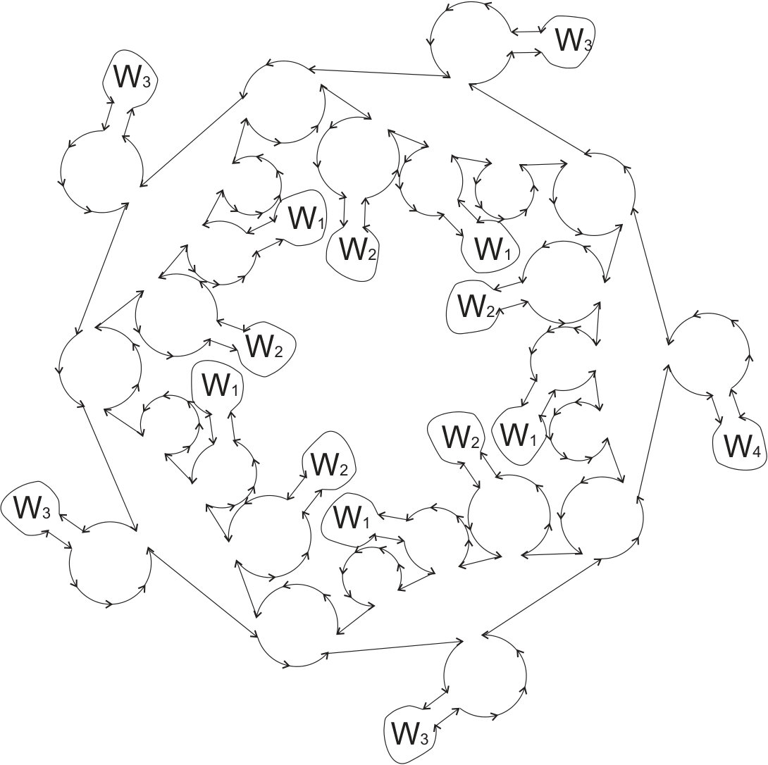 Figure 1
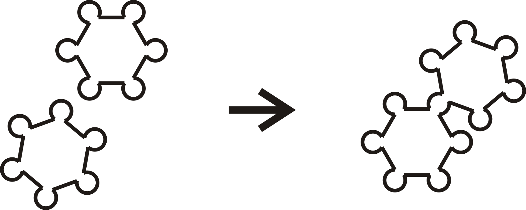 Figure 2
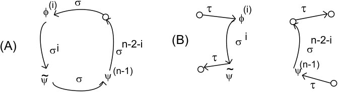 Figure 3
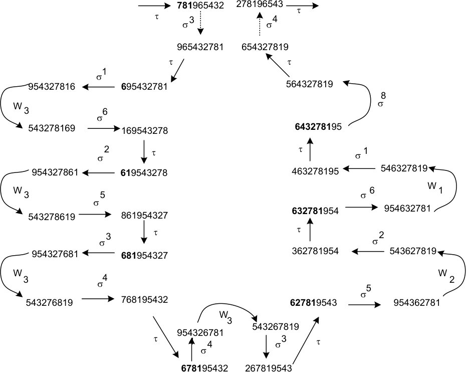 Figure 4
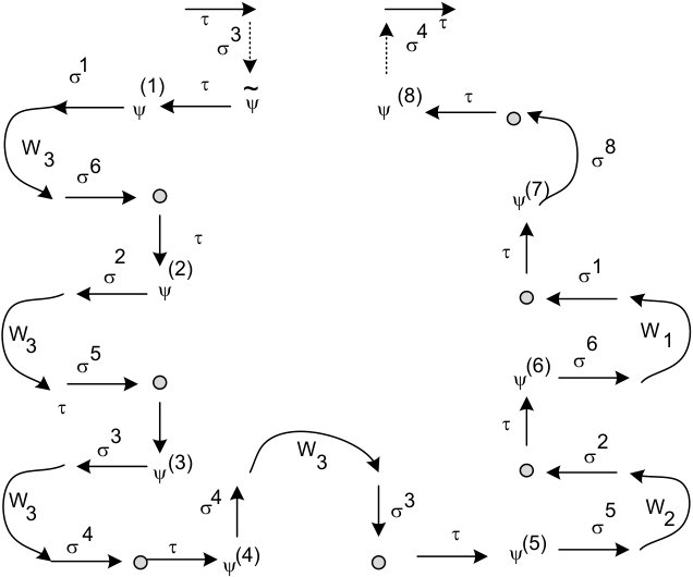 Figure 5
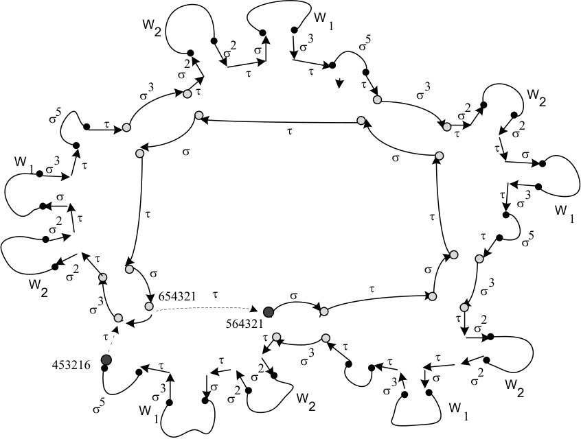 Figure 6
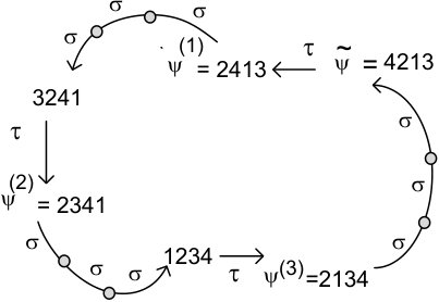 Figure 7
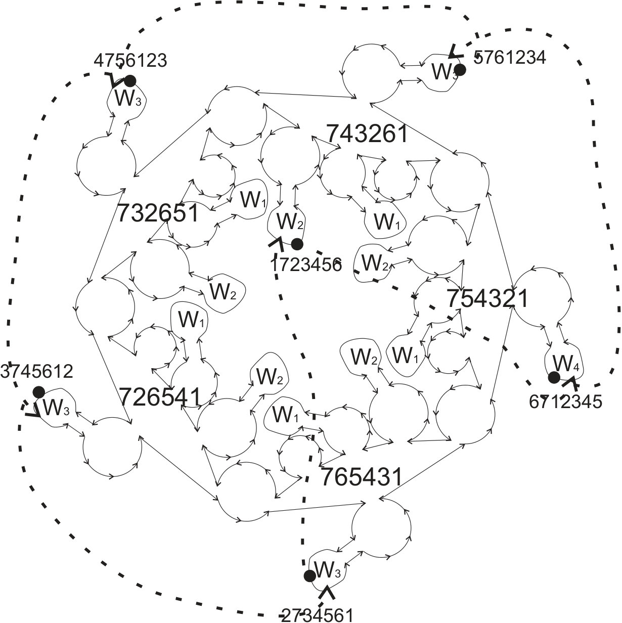 Figure 9
Peer Reviews
No public reviews on file for this paper yet. If you reviewed it on a platform where reviews are public (OpenReview, ICLR, NeurIPS, ICML), you can paste yours below so the community can read it here.
Videos
No videos yet. Explain this paper in a talk, walkthrough, or lecture? Add one.
Syntactic View of Sigma-Tau Generation
of Permutations
Wojciech Rytter
Faculty of Mathematics, Informatics and Mechanics, University of Warsaw, Warsaw, Poland
[rytter,w.zuba]@mimuw.edu.pl
Wiktor Zuba
Faculty of Mathematics, Informatics and Mechanics, University of Warsaw, Warsaw, Poland
[rytter,w.zuba]@mimuw.edu.pl
Abstract
We give a syntactic view of the Sawada-Williams -generation of permutations. The corresponding sequence of -operations, of length is shown to be highly compressible: it has bit description. Using this compact description we design fast algorithms for ranking and unranking permutations.
1 Introduction
We consider permutations of the set , called here -permutations.
For an -permutation denote:
In their classical book on combinatorial algorithms Nijenhuis and Wilf asked in 1975 if all -permutations can be generated, each exactly once, using in each iteration a single operation or . This difficult problem was open for more than 40 years. Very recently Sawada and Williams presented an algorithmic solution at the conference SODA’2018. In this paper we give new insights into their algorithm by looking at the generation from syntactic point of view.
Usually in a generation of combinatorial objects of size we have a starting object and some set of very local operations. Next object results by applying an operation from , the generation is efficient iff each local operation uses small memory and time. Usually the sequence of generated objects is exponential w.r.t. . From a syntactic point of view the generation globally can be seen as a very large word in the alphabet describing the sequence of operations. It is called the syntactic sequence of the generation. Its textual properties can help to understand better the generation and to design efficient ranking and unranking. Such syntactic approach was used for example by Ruskey and Williams in generation of (n-1)-permutations of an n-set in [3].
Here we are interested whether the syntactic sequence is highly compressible. We consider compression in terms of Straight-Line Programs (SLP, in short), which represent large words by recurrences, see [4], using operations of concatenation. We construct SLP with recurrences, which has bit description.
The syntactic sequence for some generations is highly compressible and for others is not. For example in case of reflected binary Gray code of rank each local operation is the position of the changed bit. Here and the syntactic sequence is described by the short SLP of only size:
In case of de Bruijn words of length each operation corresponds to a single letter appended at the end. However in this case the syntactic sequence is not highly compressible though the sequence can be iteratively computed in a very simple way, see [7]. In this paper we consider the syntactic sequence (over alphabet ) of Sawada-Williams -generation of permutations presented in [6, 5]. An SLP of size describing is given in this paper. The -generation of -permutations by Sawada and Williams can be seen as a Hamiltonian path in the Cayley graph . The nodes of this graph are permutations and the edges correspond to operations and .
We assume that (simple) arithmetic operations used in the paper are computable in constant time.
Our results.
We show:
can be represented by the straight-line program of size:
- •
- •
- •
where and . 2. 2.
Ranking: using compact description of the number of steps (the rank of the permutation) needed to obtain a given permutation from a starting one can be computed in time using inversion-vectors of permutations. 3. 3.
Unranking: again using the -th permutation generated by can be computed in time.
2 Preliminaries
Denote by all permutations cyclically equivalent to . Sawada and Williams introduced an ingenious concept of a seed: a shortened permutation representing a group of cycles. Informally it represents a set of permutations which are cyclically equivalent modulo one fixed element, which can appear in any place.
Let denote a modified addition modulo , where . It gives a cyclic order of elements . We write iff .
Formally a seed is a tuple of distinct elements of of the form , such that and is a permutation. The element is called a missing element.
Denote by the set of all -permutations resulting by making a single insertion of into any position in , and making cyclic shifts. The sets are called packages, the seed is the identifier of its package . One of the main tricks in the Sawada-Williams construction is the requirement that the missing element equals . In particular this implies the following:
Observation 1**.**
A given -permutation belongs to one or two packages. We can find identifiers of these packages in linear time.
The algorithm of Sawada and Williams starts with a construction of a large and a small cycle (covering together the whole graph). The graph consisting of these two cycle is denote here by . The small cycle is very simple. Once is constructed the Hamiltonian path is very easy: In each cycle one -edge is removed (the cycles become simple paths), then the cycles are connected by adding one edge to .
2.1 Structure of seed graphs
First we introduce seed-graphs. Define the seed-graph of the seed , denoted here by (denoted by in [6]), as the graph consisting of edges implied by the seed . The set of nodes consists of , the set of edges consists of almost all -edges between these nodes (except the edges of the form ), but the set of -edges consists only of the edges of the form , where is the missing element. see Figure 1.
For a seed with , let
.
For denote In other words , for , is the word right-shifted by and with added at the beginning. Observe that:
Example 2*.*
For we have
Each can be sequenced easily as a simple cycle in . Two seeds are called neighbors iff . The permutations of type play crucial role as connecting points between packages of neighboring seeds.
Observation 3**.**
*Two distinct seeds are neighbors iff , and after removing both from and the sequences become identical.
2.2 The pseudo-tree of seeds
For a seed denote by the maximal length of a prefix of such that for . For example (here the missing number is 5). For each two neighbors we distinguish one of them as a parent of the second one and obtain a tree-like structure called a pseudo-tree denoted by . If and we write . Additionally if we write and we say that is the -th son of .
The function gives the tree-like graph of the set of seeds, it is a cycle with hanging subtrees rooted at nodes of this cycle. The set of seeds on this cycle is denoted by . For example
Due to Lemma 5 we have:
Observation 4**.**
If then all -edges of are in .
For let be the subtree of rooted at including and nodes from which is reachable by -links.
2.3 A version of Sawada-Williams algorithm
We say that an edge conflicts with iff . Non-disjoint packages can be joined into a simple cycle by removing two -edges conflicting with -edges.
By a union of graphs we mean set-theoretic union of nodes and set-theoretic union of all edges in these graphs.
Denote by the graph in which we removed all -edges conflicting with -edges. The -edges have priority here. A version of the construction of a Hamiltonian path by Sawada-Williams, denoted by , can be written informally as:
**Algorithm ** Compute ;
remove from all -edges conflicting with -edges in
; add to the edge
remove edges
return { is now a Hamiltonian path }
Lemma 5**.**
.
Proof.
To prove that the paths are the same it is enough to prove that both begin in the same place and that edges are used from exactly the same vertices. The particular Hamiltonian path in [6] is described in terms of a function , which for any vertex assigns a next one on the path (by returning or ). The function for a given permutation produces a -edge when (unless or ), where is cyclically first element after jumping over (equal to if ).
The condition of being equal to in permutation is exactly the same condition as being the missing element of a seed such that (for one of two seeds if ). For a permutation such that the missing element of happens to be the first element of the permutation if and only if . is a set of those permutations from , whose ingoing edge in is a -edge. As -edges exchange the first two elements hence both approaches describe the same sets of edges (unless belongs to the ). If the permutation belongs to the package for a hub seed , the only difference from the previous case is that it can belong to the first part of the path of length (including the special permutation ).
The first permutations (the ones that are cyclically equivalent to after removing element which appears on first or second position) generate the same pattern in both constructions (alternation of and edges). All other permutations from those packages follow the same rules as the ones from packages corresponding to seeds with height , with the difference that permutations are not explicitly named (and that play a different role being the ones from the beginning of the path). In this way we have shown that . ∎
3 Compact representation of bunches of permutations
Our aim is to give a syntactic version of : the sequence of -labels of represented compactly. We have to investigate more carefully the structure of seed-graphs and their interconnections. We introduce the basic components of : groups of permutations corresponding to a subtree of seeds which are not on the cycle in the pseudo-tree. For define
[TABLE]
In other words connects with the ”outside world”, only through .
We start with properties of local interconnection between two packages.
Lemma 6**.**
* ** Two seeds are neighbors iff one of them is the parent of another one. If then is the -cycle containing both and , for some , and has a structure as shown in Figure 2(A), where is the -th son of . If then . Furthermore exists for all .*
Proof.
Assume that . Without loss of generality we can assume that (as cyclically equivalent permutations belong to the same packages). After removing any element from the first element after is either or in both cases we obtain a valid seed if and only if the removed element is greater by one than that element following . When removing element we always receive a seed which package contains and if we remove this is only the case if . It means that if then one of those seeds (denote it by ) is equal to (without an element ) and the other (denote it by ) to . Removing both elements from gives us the sequence obtained from and after the appropriate removals.
Permutations and are cyclically equivalent. If and then elements form a sequence decreasing by one: a sequence with a property and ( if ).
We obtain seed by removing the element from and inserting the element (between elements and ). The removal shortens the decreasing sequence by 1 and the insertion can neither shorten it (as the element lands outside of the sequence) nor extend it (even if as for the pair would have to be equal to which is impossible outside of ). Hence
[TABLE]
If then the decreasing sequence is formed by elements (omitting element ). The removal of decreases the length of the sequence by 1 and insertion of cut it just before that element. We have
[TABLE]
We can remove from the seed and insert in any of the places after obtaining a valid seed which is a son of .
Hence we know that packages of two seeds intersects if and only if they are in a parent-son relation, and that every seed of height greater than 1 has exactly seed-sons. We can also easily check which son of the seed is or compute for any . ∎
For and a seed of height we define as the sequence of labels of a sub-path in starting in and ending in . In other words it is a -sequence generating all -permutations (each exactly once) of .
Observation 7**.**
By Lemma 6 every seed such that has exactly sons whose heights depend only on height of . Hence (by induction on heights) all trees are isomorphic for seeds of the same height. Consequently the definition of is justified as it depends only on the height of .
For a permutation and a sequence of operations denote by the set of all permutations generated from by following , including .
The word satisfies:
In this section we give compact representation of
For example if then is a traversal of except cyclically equivalent permutations, common to and , where .
Recall that we denote
Theorem 8**.**
For we have the following recurrences:
**
Proof.
Assume is of height , then by Lemma 6 the first, from left to right, children of in the subtree are of height and the next children are of heights . The representative of the -th son of equals (see Figures 3 and 4 ). ∎
4 Compact representation of the whole generation
We have the following fact:
Observation 9**.**
*Assume two seeds satisfy: and
. Then if and then .*
Theorem 10**.**
The whole -sequence starting at , ending at , and generating all -permutations, has the following compact representation of size (together with recurrences for ):
Proof.
For every non-hub seed we had that , where . The only difference for a hub seed is that cannot be considered as part of a tree rooted at (with already defined -links), since and this would lead to a cycle ( is reachable via parent-links from ). Thus to prevent this problem we define as with the part corresponding to the first son removed (leaving only the part), and also delete the last symbol , as it does not appear at the end of the path (it corresponds to one of the -edges removed when joining two cycles into one path). Now consists of such segments (corresponding to hub seeds) joined by -edges (they are linked in the same way as if the previous part was a son of the next one). Additionally it starts with -path representing the small path with the last -edge replaced by a -edge. ∎
5 Ranking
We need some preprocessing to access later some values in constant time.
Observation 11**.**
All the values and for can be computed in total time and accessed in time afterwards.
The ranks of representatives of hub seeds are easy to compute. For example for we have (see Figure 5):
Lemma 12**.**
*For a given permutation we can compute in time
(a) if ,
(b) if for some .*
Proof.
By the starting path we mean the sequence on the first permutations of , see Figure 5.
(a) Given a permutation we define as permutation cyclically equivalent to and starting with , and let be the position such that . If , then
Now we distinguish two cases depending on the position of in .
Case 1: if , then
(it appears in the part of ),
Case 2: otherwise
(it appears in the part).
If , then
[TABLE]
Using similar arguments as before we have that:
if and
otherwise.
(b) If the permutation after removing is cyclically equivalent to and appears on the first position ( belongs to the starting path) then , and if it appears on the second position then , where are the first two positions of .
Otherwise we define , and like in case (a) and . We know that , and want to compute minus the rank of the first permutation of which appears in with rank greater than . That permutation is equal to
[TABLE]
(equal to if was defined for hub seeds in the same way as for the other ones), and has rank equal to
[TABLE]
If then else if then
[TABLE]
Otherwise we have
[TABLE]
Those two algorithms lets us rank permutations in basic cases, and allows us to reduce the main problem to a simpler one (ranking the representatives of seeds). ∎
Hence we concentrate on ranking permutations of type (representatives of seeds). We slightly abuse notation and for a seed define .
For a non-hub seed denote by the highest non-hub ancestor of and let . Observe that the anchor is the first contacting seed with the hub, it is the first ancestor of such that for some , in fact for .
for a non-hub seed , can be treated as its distance from . It happens that computing the rank of the anchor is much easier, since we have to deal only with the hub seeds. The bottleneck in ranking is computation of the distance of a seed representative from . Define:
Denote also by the position of in counting from the end of sequence . For example for we have , since and 8 is on the 5-th position from the right.
Observation 13**.**
* ** If and is the -th son of then *
Example 14*.*
Let , then . The path from to is
[TABLE]
see Figure 3. Its length equals , we have:
Observation 15**.**
* iff is the -th son of .*
For the parent-sequence denote
For a seed define the decreasing sequence of , denoted by , as the maximal sequence , where such that for . Denote . The length of the parent-sequence from to its anchor is .
Example 16*.*
We have: . Hence the path from to is of length . This path equals:
We have: , .
The key point is that we do not need to deal with the whole parent-sequence, including explicitly seeds on the path, which is of quadratic size (in worst-case) but it is sufficient to deal with the sequence of orders of sons, which is an implicit representation of this path of only linear size
Lemma 17**.**
For a non-hub seed we can compute and in time.
Proof.
We know the length of the parent sequence from to its anchor, since we know . Now we use the following auxiliary problem
Inversion-Vector problem:
for a seed compute for each element the number
of elements smaller than which are to the right of in .
Assume . We introduce a new linear order
.
Then we compute together the numbers w.r.t. linear order for each element in .
Now is computed separately for each in the following way:
, where
The Inversion-Vector problem can be computed in time, see [1]. Consequently the whole computation of numbers is of the same asymptotic complexity. We know that , where and we know also which son of is . This knowledge allows to compute within required complexity. This completes the proof. ∎
Corollary 18*.*
For a non-hub seed the value can be computed in time.
Proof.
Let the parent-sequence from to its anchor be
where .
Then and
, which allows us to compute in time:
Now the thesis is a consequence of Observation 11, Observation 13 and Lemma 17. This completes the proof. ∎
Example 19*.*
(Continuation of Example 16) For from Example 16 we have:
The following result follows directly from Corollary 18, Lemma 12 and Observation 11.
Theorem 20**.**
[Ranking]* For a given permutation we can compute the rank of in in time *
6 Unranking
Denote by the -th permutation in , and for let (it is the -th permutation in , counting from the beginning of this bunch). The following case is an easy one.
Lemma 21**.**
*If we know a seed together with its rank, such that
, then we can recover in linear time.*
Proof.
Let , and . In linear time we find such that .
If , then does not belong to (it belongs to ).
If , then is equal to rotated by to the right, and if , then it is the same permutation rotated by to the left.
In this way we reduced the problem of unranking permutation outside of to finding a package containing the permutation. ∎
We say that a permutation is a hub-permutation if for some .
Lemma 22**.**
*We can test in time if is a hub-permutation.
***(a)***If ”yes” then we can recover in time.
(b) Otherwise we can find in time an anchor-seed together with such that .*
Proof.
If then is equal to rotated to the left by , with inserted on first position if is odd, and on the second if it is even.
Otherwise let (we use integer division), and let
[TABLE]
(with substituted by if equal to [math]). belongs to , or to , where .
If then equals to rotated to the left by .
In the other case in linear time we find such that
[TABLE]
[TABLE]
If then is equal to rotated to right by , else if , then is equal to rotated to the left by . Otherwise , and it is not a hub-permutation.
By using this algorithm we either already succeed in finding the right permutation, or restrict ourselves to a limited regular part of . ∎
For a sequence of positive integers denote
The sequence is called here –stably increasing iff
, and .
Lemma 23**.**
* *
(a)* Assume we have a –stably increasing sequence of length . Then after linear preprocessing we can locate any integer in the sequence in
time.
(b) The sequence , where is –stably increasing.*
Proof.
(a) Denote , and let be a sequence such that .
It can be computed in linear time by scanning the sequence from left to right and reporting whenever element exceeds next power of .
Thanks to the fact that sequence is –stably increasing the maximal difference between consecutive values of a sequence is bounded by .
When locating in the sequence we can compute the value
[TABLE]
It now suffices to binary scan the part of sequence between positions and , which has a length bounded by .
(b) For any the value of equals
[TABLE]
[TABLE]
We have:
[TABLE]
[TABLE]
[TABLE]
Combining those two parts of the lemma allows us to locate values in the sequence in time after linear preprocessing dependent only on the value of . ∎
Lemma 24**.**
After linear preprocessing if we are given a height of a non-hub seed , and a number we can find the number and of the seed-son of such that in time if .
Proof.
Let . We need such that . For we have , hence if the simple division by suffices to find the appropriate . Otherwise we look for such that
[TABLE]
Let
By Lemma 23(b) is –stably increasing (it is a prefix of for which we made the linear preprocessing). Hence by Lemma 23(a) we can find the required in time.
Moreover if , then , where has height . Otherwise . ∎
Theorem 25**.**
[Unranking]* For a given number we can compute the -th permutation in Sawada-Williams generation in .*
Proof.
From Lemma 22 we either obtain the required permutation (if it is a hub-permutation) or obtain its anchor-seed and . In the second case we know that and it equals . Now after the linear preprocessing we apply Lemma 24 exhaustively to obtain for a seed such that . However we do not know and have to compute it.
Claim 26*.*
If we know and then can be computed in
time.
Proof.
We can compute the second element of as and as where is the second element of , and . Then we use the order:
.
We produce a linked list initialized with . For we want to insert after position from the end of the current list (all the smaller elements are already in the list and we know, that after there are such elements). is composed of and consecutive elements of the final list. The data structure from [2] allows us to achieve that in time. ∎
Finally we use this claim and Lemma 21 to obtain the required permutation . ∎
7 Examples of ranking and unranking
We show on representative examples how the ranking and unranking algorithms are working.
Ranking.
When ranking we first find a permutation cyclically equivalent to and then a seed whose package contains both and (in case of two candidates for we choose the parent). We have . Next we compute by computing inversion vector of . After that we compute and
[TABLE]
[TABLE]
[TABLE]
Now it is enough to compute (knowing that belongs to the hub), which again is computed in two steps – rank of the first permutation of (outside of the starting path) is equal to and occurs permutations later. After summing all the values our final output is:
Unranking.
Forget now that we already know the permutation with rank 1584702. When looking for a permutation with rank we first check if is not in the starting path () and then after subtracting from we divide it by , to get . We now know, that the permutation belongs to .
We have
[TABLE]
hence we know, that the permutation belongs to the part of . We decrease the rank by to get .
Then we descend down the seed tree by choosing the fifth son, because , with the remaining rank . Next we go to the third son since , with the remaining rank equal .
In the next step we know that , and also that , hence further descent is not needed.
In this moment we came to an unknown seed for which we know , and . Using Claim 26 we recover . Now we know that the required permutation is in , and it equals , then we use Lemma 21 to obtain , and this permutation is our final output.
8 Cyclic -sequence
A -sequence of permutations is cyclic if the last permutation is equal to the first one. Sawada and Williams in [5] have given an iterative construction of a cyclic -sequence. They have shown how to partition the graph of permutations into two edge disjoint cycles (2-cycles cover) of respectively inner and outer cycles. Below we give an example of this structure for .
We define ”switches” as permutations of the form
[TABLE]
for . In other words they are cyclic shifts of the identity permutation in which is inserted into the second position.
Observation 27**.**
There is a one switch on the inner cycle and switches on the outer cycle.
8.1 Sawada Williams construction of Hamiltonian cycle.
The algorithm basically computes the cycles , then the switches are appropriately ordered as . Afterwards the outgoing edges for the switches are redirected by choosing the outgoing -edge (in the 2-cycle cover these were -edges). More explicitly we redirect:
for each redirect , additionally redirect .
8.2 Two cycles construction
Let denote a modified addition modulo , where . It gives a cyclic order of elements , with attached element (). For we write and .
Lemma 28**.**
The outer sequence is represented (after removing one edge) by the linear sequence
[TABLE]
and the inner sequence is represented by the linear sequence , where
[TABLE]
Proof.
First we need to prove, that for outside of hub
[TABLE]
for and defined as before, but after replacing with . For the ordering of elements (which element is considered missing in the seed, and thus equal to or ) is in fact inherited from the parent seed (the first elements after in the permutation), thus there is no change from the proof of 8. For (the cycle of permutations which belong to for just one ) the missing element is inserted just after , thus there can be no further descent in the tree of seeds and at the same time there is only one permutation in the cycle for which the SW function gives a -edge.
Every hub seed has one child which is also a hub seed. In the previous construction it was always . In this construction it is as hub seeds are those of a form . Hence the construction divides the first son from sons to (and the cycle with ). The outer cycle covers the first sons of hub seeds, and the inner cycle covers the remaining ones. Son of each hub seed have height with one exception – seed which is the first son of a hub seed has height . Hence the outer cycle has the stated representation (additional represents transition to the second son – next hub seed). In the inner cycle each child of hub seeds has the same height as in the previous construction () and are visited in the same order. After all those children are visited there appears which represents the ”return to the parent seed” (thus in this cycle hub seeds are visited in the reversed order). ∎
8.3 Alternative path construction
Claim 29*.*
In the path obtained with the new method the sequence representing it is equal to
[TABLE]
(with the last removed) It is equal to the concatenation of representations from Lemma 28 with the ending removed in both representations and with added between them.
Lemma 30**.**
In the new path we can rank a permutation in time and unrank it in .
Proof.
Ranking algorithm in the previous construction contained four parts:
Counting for in . 2. 2.
Computing for a given in . 3. 3.
Counting out of in . 4. 4.
Ranking inside the hub in .
With a few minor changes we can adjust it to the new path construction.
The first part does not really change (it is enough to know what are the missing elements in the seed and its children).
In the second part the only difference is that in the order used in inversion vector problem we must insert element somewhere. As it is never a missing element, we can insert it as a minimal element (or leave the order untouched if ).
The third part is identical.
The biggest difference occurs in the fourth part – we first need to determine to which cycle from the two cycle construction it belongs to. The permutation belongs to the outer cycle when it belongs to perms of two seeds , where , and either , or ( and it is one of three first permutations in the cycle). In this case we must rank the permutation in relation to (rank in + (or ) unless it is or ) and add
[TABLE]
(where ) if , and if .
Otherwise it belongs to the inner cycle. In this case we rank it like in the normal construction (in relation to the first permutation in ), then we subtract (or ) and add
[TABLE]
.
Unranking algorithm contained four parts as well:
Finding appropriate tree of seeds (or returning permutation if it belongs to hub) in . 2. 2.
Computing and in . 3. 3.
Obtaining out of in . 4. 4.
Unranking in in .
Parts 2,3,4 remain unchanged (the only change is the use of instead of ).
In the first part we first
[TABLE]
if that is the case we check if (we unrank in the part with ) and if that is not the case we divide by (using integer division) and unrank it in appropriate three of seeds.
[TABLE]
we unrank in the inner cycle – we divide by (using integer division) and proceed as in the previous algorithm. ∎
8.4 Polynomial construction for the cycle
Lemma 31**.**
There exist an SLP for Hamiltonian cycle of size .
Proof.
Switch for . For , and , thus each (or ) on the outer cycle contains one such switch. For and , thus the remaining switch belongs to one of the parts of the inner cycle.
We can divide each such part into two – the one before the switch and the one after it. Each such part can be represented by an of size as a word can be divided at most once for each and (each other does not contain a switch, thus remain undivided). ∎
Lemma 32**.**
We can rank and unrank in the cycle in .
Proof.
Scheme of algorithm:
We count ranks for all the ”switches” in the path in . Then we count differences between ranks of two next ”switches” (in the order of the path) and ranks of switches in the cycle (iterating through switches in the order of the cycle) in total time and space.
Rank:
Rank permutation in path in . 2. 2.
Find last ”switch” with smaller or equal path rank, and count the difference (if rank is smaller then the rank of first switch we count everything modulo ) in . 3. 3.
Add the difference to cycle rank of that ”switch”.
Unrank:
Find last ”switch” with smaller or equal cycle rank and count the difference in . 2. 2.
Add the difference to path rank of that ”switch”. 3. 3.
Unrank in the path with the new value in .
∎
8.5 Efficient construction for cycle
Lemma 33**.**
Routes of (seeds which perms contain) ”switches” are always of the form with [math] or element erased (for example for ) or are equal to . Furthermore we can compute all the ranks of ”switches” on the new path in total time.
Proof.
Each ”switch” belongs to perms of just one seed namely for ().
When going through parent edges until reaching each time the missing symbol is inserted after shifting all elements till by one, and erasing the element just after it (jumping over element ). Hence each time parent edge is used we erase element closer to right by one with the exception of the one time when appears just after for the first time. In that case the element erased next is closer to the right by two. Thus each route is built of numbers decreasing by ones (sometimes with one number missing). Each time the height of the tree rises by exactly one.
When , then , thus the route ends with .
If then , thus is never jumped over. As we start in a seed with tree of height , (this is the switch which appears in the part).
If , then is jumped over at the -th step from resulting in .
When the jump over appears inside , and thus does not touch .
When (this is the switch from in the inner cycle).
When appears on the -rd place of -nd (last) cycle in . When the jump over appears inside and thus appears on the -th place of -rd cycle in .
As the heights of trees grow always by
[TABLE]
For these two values for and differs by
[TABLE]
Hence all the can be counted in total time (we get 4 cases - each counted in (see Lemma 18), plus time to compute the other ones by adding the differences). Each is the first in a part of the sequence ( or ), thus all can be counted in total time. ( or for ). ∎
Theorem 34**.**
-cycle from [5] has a SLP representation.
Proof.
Each tree of seeds in the outer cycle (and one in the inner) is divided into two parts. Each tree is divided differently, but in each the division happens either in the last part, or the penultimate one, thus it is enough to divide the definitions of into three parts , and for each tree divide one of the words.
More precisely for () let:
[TABLE]
[TABLE]
[TABLE]
The division of the tree with for :
[TABLE]
[TABLE]
[TABLE]
[TABLE]
[TABLE]
[TABLE]
∎
Theorem 35**.**
In the cycle we can rank in time and unrank in time.
Proof.
We use the algorithm from 32, just count ranks of ”switches” in total time. ∎
The reference list from the paper itself. Each links out to its DOI / PubMed record.
- 1[1] Timothy M. Chan and Mihai Patrascu. Counting inversions, offline orthogonal range counting, and related problems. In Moses Charikar, editor, Proceedings of the Twenty-First Annual ACM-SIAM Symposium on Discrete Algorithms, SODA 2010, Austin, Texas, USA, January 17-19, 2010 , pages 161–173. SIAM, 2010.
- 2[2] Paul F. Dietz. Optimal algorithms for list indexing and subset rank. In Algorithms and Data Structures, Workshop WADS ’89, Ottawa, Canada, August 17-19, 1989, Proceedings , pages 39–46, 1989.
- 3[3] Frank Ruskey and Aaron Williams. An explicit universal cycle for the ( n -1)-permutations of an n -set. ACM Trans. Algorithms , 6(3):45:1–45:12, 2010.
- 4[4] Wojciech Rytter. Grammar compression, LZ-encodings, and string algorithms with implicit input. In Automata, Languages and Programming: 31st International Colloquium, ICALP 2004, Turku, Finland, July 12-16, 2004. Proceedings , pages 15–27, 2004.
- 5[5] Joe Sawada and Aaron Williams. Solving the sigma-tau problem. URL: http://socs.uoguelph.ca/~sawada/papers/sigma Tau Cycle.pdf .
- 6[6] Joe Sawada and Aaron Williams. A Hamilton path for the sigma-tau problem. In Proceedings of the Twenty-Ninth Annual ACM-SIAM Symposium on Discrete Algorithms, SODA 2018, New Orleans, LA, USA, January 7-10, 2018 , pages 568–575, 2018.
- 7[7] Joe Sawada, Aaron Williams, and Dennis Wong. A surprisingly simple de Bruijn sequence construction. Discrete Mathematics , 339(1):127–131, 2016.