On the mean square displacement in Levy walks
Christoph Borgers, Claude Greengard

TL;DR
This paper analyzes the mean square displacement in Levy walks, providing new closed-form expressions and bounds, and clarifies how different components of MSD depend on step duration distributions.
Contribution
It extends existing asymptotic results by deriving explicit formulas and bounds for MSD in Levy walks using elementary analysis.
Findings
Derived closed-form expressions for MSD in Levy walks.
Identified how super-linear, linear, and sub-linear MSD components depend on step durations.
Provided bounds for MSD based on the entire distribution function.
Abstract
Many physical and biological processes are modeled by "particles" undergoing L\'evy random walks. A feature of significant interest in these systems is the mean square displacement (MSD) of the particles. Long-time asymptotic approximations of the MSD have been established, via the Tauberian Theorem, for systems in which the distribution of the step durations is asymptotically a power law of infinite variance. We extend these results, using elementary analysis, and obtain closed-form expressions as well as power law bounds for the MSD in equilibrium, and representations of the MSD as sums of super-linear, linear, and sub-linear terms. We show that the super-linear components are determined by the mean and asymptotics of the step durations, but that the linear and sub-linear components (whose size has implications for the accuracy of the asymptotic approximation) depend on the entire…
Click any figure to enlarge with its caption.
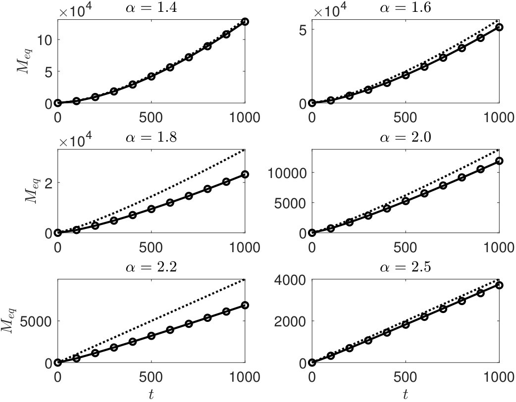 Figure 1
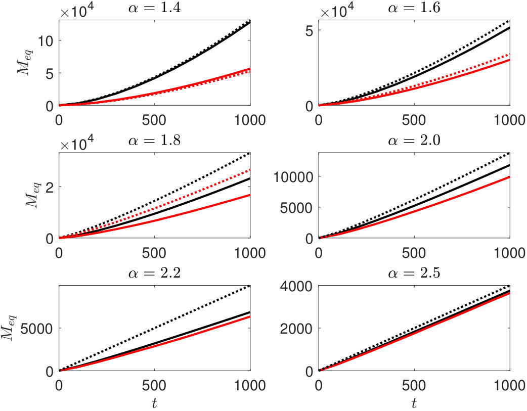 Figure 2
Peer Reviews
No public reviews on file for this paper yet. If you reviewed it on a platform where reviews are public (OpenReview, ICLR, NeurIPS, ICML), you can paste yours below so the community can read it here.
Videos
No videos yet. Explain this paper in a talk, walkthrough, or lecture? Add one.
On the
mean square displacement in Lévy walks
Christoph Börgers222Department of Mathematics, Tufts University, Medford, MA 02155. email: [email protected] and Claude Greengard333Two Sigma Investments, LP, and Courant Institute of Mathematical Sciences, New York University, New York, NY 10012. email:[email protected]
Abstract
Many physical and biological processes are modeled by “particles” undergoing Lévy random walks. A feature of significant interest in these systems is the mean square displacement (MSD) of the particles. Long-time asymptotic approximations of the MSD have been established, via the Tauberian Theorem, for systems in which the distribution of the step durations is asymptotically a power law of infinite variance. We extend these results, using elementary analysis, and obtain closed-form expressions as well as power law bounds for the MSD in equilibrium, and representations of the MSD as sums of super-linear, linear, and sub-linear terms. We show that the super-linear components are determined by the mean and asymptotics of the step durations, but that the linear and sub-linear components (whose size has implications for the accuracy of the asymptotic approximation) depend on the entire distribution function.
keywords:
Lévy random walk, mean square displacement, super-diffusion, anomalous diffusion
AMS:
60G51, 82C70
1 Introduction
We consider a random walker in moving at random velocities in straight line segments of random duration. At the end of each flight segment, a new velocity and duration are chosen at random. We assume that the durations and velocities are independent. Denote by the distribution function of the duration. When has infinite variance, the case of primary focus in this paper, this process is called a Lévy walk [20, 21, 25, 26, 30]. A swarm of random walkers starting at the same location and performing independent Lévy walks exhibits super-diffusion, that is, faster than linear growth in the mean square displacement (MSD) — the mean of the square of their distances from the origin. One finds many discussions of physical and biological applications of Lévy walks and related random processes leading to super-diffusion in the literature. Our own interest in the subject started when we modeled the evolution of a rarefied gas in an ultra-thin planar channel as a succession of infinite-variance flights and showed that the molecular density approaches a Gaussian distribution with a variance which grows super-linearly [5, 15, 23]. Other examples of applications include certain kinds of transport in fluid flow [26, 32], transport in biological cells [6, 28], the migration of bacteria [1], predator search behavior [27], and traveling humans [7]. Also, Lorentz gases [16, 33] and other billiards problems [2], in which there is no randomness in a strict sense but, rather, deterministic chaos, have been approximated by super-diffusive random walks.
The most commonly studied Lévy walks are those in which the speeds of the walkers are fixed. However, there are many interesting examples in which both the directions and the speeds of the flights are random [31]. For example, in the gas flow between horizontal plates with Maxwellian reflection conditions mentioned above, individual molecules undergo random flights whose durations and horizontal velocities are independent, with durations of infinite variance and finite expected square speed [5]. By allowing speeds to be random, but assuming that the expectation of the squared speed is finite, we include this and other examples without complicating the analysis beyond that of the single-speed case.
A fundamental quantity characterizing super-diffusion is the MSD. The common approach to analyzing the MSD is to formulate an equation describing the density of the walker location as a function of time and then to take a Fourier transform with respect to the space variables and a Laplace transform with respect to the time variable. One can then use the Tauberian theorem to deduce the long-time asymptotics of the MSD from the behavior of derivatives with respect to the Fourier variable near 0 [19, 21, 29].
An alternative and more elementary approach is to express the MSD as an integral over the velocity auto-correlation, and evaluate or analyze the integral; see for instance [2, 12]. We present a mathematical analysis of the basic properties of the MSD, using this approach, under the assumption that has finite expectation.
While the standard approach is very useful in providing insights into various aspects of the asymptotic behavior of Lévy walks, the more elementary approach taken in this paper allows the derivation of exact, explicit expressions, valid for all times, for the MSD, for important classes of problems (Section 4). This enables detailed understanding of the accuracy of asymptotic approximations for the MSD (Section 6). In other examples, when exact expressions cannot be obtained, our approach permits the derivation of time-dependent bounds, valid for all times (Corollary 7.4).
We will distinguish between the “equilibrium” MSD, , and the “transitional” MSD, . Precise definitions are given in Section 2. The difference between the two cases lies in the interpretation of “”. In the equilibrium case, should be thought of as the time at which we start watching a random walk that has been going on for a long (strictly speaking, infinite) time. In the transitional case, the walk begins at time . The equilibrium case is easier to analyze since the MSD is then expressible as a simple convolution integral, and we focus on this case.
Long-time asymptotic approximations have been derived for various duration distributions, for both and . These approximations depend only on the tails of the distributions. However, accuracy of the asymptotic approximation may only emerge after an extremely long time. For instance, if is proportional to to leading order, as occurs in numerous applications [2, 14, 33], there is typically a correction term of order . For this term to become negligible, must become small, so must be extremely large. We show that the presence or absence of a linear correction term depends on the entire distribution , not just on its tail. Similarly we show that the presence of a logarithmic factor in may cause to consist, to leading order, of a sum of two terms that only differ by a factor proportional to . Highly precise and complete knowledge of may therefore be needed to ascertain whether leading-order long-time asymptotic approximations for are accurate approximations to the actual at times of physical interest.
Of course, distributions found in real-world applications need not be exactly power laws asymptotically. We show that the model is robust in the sense that for distributions bounded by power laws, the MSDs also satisfy related bounds.
We relate the transitional MSD, , to the equilibrium MSD, . Our results on are weaker than those on and mostly concern the leading-order asymptotic behavior, but we also give a result on correction terms for . Finally, we present the asymptotic MSD for free molecular flow in planar channels [5].
2 Background and notation
Let , , be random variables with
[TABLE]
We will consider a random walker changing velocities at times . We assume that the increments , , are independent and identically distributed positive random variables. The equilibrium and transitional cases differ in the choice of distribution of , as discussed below.
Let denote the distribution of the . We assume throughout this paper that is continuous and that its mean, , is finite:
[TABLE]
Our primary concern is this paper is with the case when the second moment of ,
[TABLE]
is infinite.
At each time a new velocity vector, , is chosen. For simplicity of exposition, we will often refer to the times as ”collision” times, thinking of a particle colliding with a background. Thus the random selection of a new is thought of as the result of a “collision”. We assume that the velocities are identically distributed and independent of each other and of the collision times. We’ll also assume that the mean velocity is zero, since if it were not, one could simply subtract the mean velocity and consider the shifted velocities (the only change would be a drift in the direction of the mean velocity). Denote by the characteristic speed,
[TABLE]
where denotes the Euclidean norm. As we shall see below, given a duration distribution , the MSD is proportional to . This is the only dependence of the MSD on the velocity distribution. So, for example, given , walks in dimensions with post-collision velocities uniformly distributed on the sphere of radius and those which go only in axial directions, with equal probabilities, at speed , have identical MSDs — not just asymptotically, but for all time.
We consider two choices of :
Transitional case: . 2. 2.
Equilibrium case: is random and independent of the , with distribution function
[TABLE]
To review the significance of the distribution , recall [17] that for any ,
[TABLE]
is called the residual life at time . Denote its distribution function by , , so that for , ,
[TABLE]
Lemma 1**.**
If is continuous, then is a continuous function of .
Proof.
Let , . Let and be numbers with and . We must prove that as . We will consider the case and . The cases when one or both of and are negative can be understood analogously.
We have
[TABLE]
and therefore
[TABLE]
Similarly,
[TABLE]
and therefore
[TABLE]
[TABLE]
It therefore suffices to prove now that for any ,
[TABLE]
To prove (5), we write, for any ,
[TABLE]
Because is continuous, the right-hand side of (6) converges to as . This implies
[TABLE]
The assertion now follows because as . ∎
The importance of lies in the following well-known result from renewal theory [17, Chapter XI, Section 4].
Theorem 2**.**
In the equilibrium case,
[TABLE]
In the transitional case,
[TABLE]
We will use the following elementary fact.
Lemma 3**.**
If , then .
Proof.
Let denote a random variable with distribution function . Let denote the underlying probability space. For , let if , and otherwise. Then
[TABLE]
The integrand converges to zero as for any fixed , and is bounded by the integrable function . The Lebesgue dominated convergence theorem implies the assertion. ∎
Some simple properties of that will be of use to us later on are collected in the following lemma.
Lemma 4**.**
- (a)
If is continuous, then is continuously differentiable, with density
[TABLE] 2. (b)
If then as . 3. (c)
The expectation of is , regardless of whether is finite or infinite.
Proof.
(a) follows from the fundamental theorem of calculus.
(b) Since this follows from Lemma 3.
(c) The expectation of is
[TABLE]
Using part (b), we see that this equals . ∎
Now define the random, piecewise constant velocity, ,
[TABLE]
Consider a random walker in starting at and moving with velocity at time . The position of the random walker at time is
[TABLE]
The mean square displacement (MSD) is the quantity
[TABLE]
As mentioned in the introduction, we use subscripts to distinguish the equilibrium and transitional cases, writing and and referring to as the equilibrium MSD, and to as the transitional MSD.
3 Integral representations and properties of the MSD
3.1 The MSD as a double integral
The MSD can be expressed as an integral as follows [12]. For all ,
[TABLE]
Recalling that expectations are integrals over the sample space and using Fubini’s theorem, we conclude that
[TABLE]
The auto-correlation that appears in (7) is related to the residual life distribution as follows. Assume that . If there is no with , an event of probability , then and so . If there is a with , then and are independent and . Hence,
[TABLE]
[TABLE]
for all .
3.2 Properties of the MSD
We record the following general consequences of eq. (9).
Proposition 5**.**
In both the equilibrium and transitional cases,
- (a)
* as ,* 2. (b)
* is continuously differentiable,* 3. (c)
* for all ,* 4. (d)
* grows at least linearly, i.e., * 5. (e)
for any fixed ,
Proof.
(a) means
[TABLE]
and this holds because
[TABLE]
as . (b) follows immediately from (9) because is a continuous function (Lemma 1). In fact,
[TABLE]
Note that is a non-negative continuous function of and which tends to 1 as . Thus, for all , establishing (c). To prove (d), we will prove the existence of a positive lower bound on , valid for sufficiently large . Let and . Then
[TABLE]
as . For sufficiently small , we have . Choose so that this holds. Then for sufficiently large ,
[TABLE]
This implies (d). To prove (e), first note because of (c). Furthermore,
[TABLE]
Hence, , and, since by (d), (e) follows. ∎
3.3 Computing from
As we have seen in Theorem 2, in the equilibrium case, for all . Hence, eq. (9) becomes
[TABLE]
We now establish two consequences of this integral expression which will allow us both to construct illustrative examples and to establish the asymptotic behavior of the MSD. First, differentiating (10) and introducing the change of variables , we find
[TABLE]
Equation (11) implies, by anti-differentiation, a representation of as a single integral:
[TABLE]
Integrating by parts in (12), using (2), we obtain an integral expression for directly in terms of rather than :
Proposition 6**.**
For all , the equilibrium MSD can be expressed as
[TABLE]
Proposition 6 will prove useful in deriving asymptotic results. We now derive an alternative characterization of , which will prove useful in constructing examples. Differentiating eq. (11), we obtain
[TABLE]
Differentiating a third time, we arrive at the following proposition.
Proposition 7**.**
* is three times continuously differentiable and for all ,*
[TABLE]
with boundary conditions,
[TABLE]
It may appear at first sight that is over-determined by the four conditions in (16). However, note that (15) implies that Therefore, and are equivalent conditions.
4 A family of power laws with closed-form
A standard assumption in the literature is that is, asymptotically, a power law. This enables derivation of asymptotic behavior of Lévy walks, including the MSD, via Laplace transforms and the Tauberian theorem [21].
However, in the equilibrium case, for a variety of power laws, one can get a more precise result — the exact MSD for all times. For example, for and , let
[TABLE]
The mean of this distribution is
[TABLE]
For , the second moment of is infinite, while for , it is finite. Using (18), we see that in the limit as , with fixed, we obtain the exponential distribution
[TABLE]
We also note that
[TABLE]
Using either Proposition 6 or Proposition 7, we can compute exactly for the distributions in (17) and (19). For example, consider the case . Using eqs. (15) and (18), we obtain
[TABLE]
Integrating, using the boundary conditions (16), we find
[TABLE]
[TABLE]
and
[TABLE]
This proves eq. (22) below. The other parts of Proposition 8 are proved by similar straightforward calculations.
Proposition 8**.**
For the distribution given by (17) if , and by (19) if , we have, for all ,
[TABLE]
We stress again that these are exact formulas valid for all times, not just asymptotic ones. Note that (20) tends to (21) as , and to (22) as . Using (18), it is also straightforward to see that in the limit as with fixed, (20) tends to (23).
When the particles move at a constant speed , there is a sharp front consisting of particles which have experienced no collisions. Then at time , the probability of having experienced no collisions is and the contribution to of this front is . For the above power law with , this gives a contribution of
[TABLE]
As , the front contributes an asymptotically constant proportion to the total MSD:
[TABLE]
For , the contribution of the front to becomes negligible as .
5 Leading-order asymptotics of
If has finite variance, then
[TABLE]
by eq. (11) together with Lemma 4, part (c). Hence,
[TABLE]
The more interesting case is that of infinite variance, to which we now turn. In several places we will make use of the following lemma.
Lemma 9**.**
Let and be non-negative, locally integrable functions of with and for sufficiently large ,
[TABLE]
and
[TABLE]
Then
[TABLE]
Proof.
Let . Choose so that for , Then for ,
[TABLE]
Therefore
[TABLE]
Letting , we find
[TABLE]
By a similar argument,
[TABLE]
Since these conclusions hold for any , the assertion follows. ∎
The following theorem shows that in the infinite variance case, the leading-order long-time asymptotic behavior of is determined by the leading-order long-time asymptotic behavior of .
Theorem 10**.**
Let and be infinite-variance distributions with finite means and and equilibrium MSDs and , respectively. Assume that
[TABLE]
Then
[TABLE]
Proof.
, and , imply
[TABLE]
as . From Lemma 4, part (c), and eq. (11), we know that and tend to as . This implies, using Lemma 9, that
[TABLE]
Because and tend to , this in turn implies, again by Lemma 9,
[TABLE]
which is the statement of the theorem. ∎
Proposition 8 and Theorem 10 together imply the well-known formulas [3, 24] for the leading-order asymptotic behavior of for , summarized in the following corollary. We add to the statement of this corollary the result for the finite variance case (see eq. (24)).
Corollary 11**.**
Suppose that
[TABLE]
for some and . Then as ,
[TABLE]
6 Accuracy of leading-order asymptotics: Examples.
In this section we explore the accuracy of leading-order asymptotic descriptions of such as those given in Corollary 11.
6.1 Canonical power laws
For the power laws
[TABLE]
discussed in Section 4, the accuracy of the leading-order asymptotics can be ascertained from eqs. (20)–(22). The discrepancy between the exact and the leading-order asymptotics given in Corollary 11 is for , and for . Therefore the leading-order asymptotic approximation for is inaccurate when unless is very large.
Figure 1 illustrates this conclusion, using , , and six different values of . The figure shows, for , the exact (solid), the leading-order approximations (dotted), and Monte Carlo estimates of (circles), based on 500,000 simulated random walkers for each value of .
For , the relative difference between and its leading-order approximation is approximately , and for this to be smaller than 0.05, corresponding to 5% accuracy, we need . Zarfaty et al. [33] relate slow convergence of to slow convergence in the Central Limit Theorem (CLT) for [22], a special case of slow convergence for any slowly varying scaling in the generalized CLT [4]. A related, deterministic, problem is that of infinite-horizon billiards, in which the asymptotic MSD also contains a logarithmic factor. For this case, Cristadoro et al. derived the first two terms in the asymptotic expansion of the MSD [9] and demonstrated numerically that the leading-order term is a poor approximation of the actual MSD for reasonable lengths of time [10]. In [11], the same authors derived an evolution equation for the MSD for random walks on a lattice with exponentially distributed waiting times between flight segments, a problem that can be seen as an abstraction of the infinite-horizon Lorentz gas when .
6.2 A general approach to constructing examples
Instead of beginning with and computing , we can also, for the purposes of constructing interesting examples, start with and compute from it, based on the following proposition.
Proposition 12**.**
Let . There exist an expected speed and a continuous probability distribution function on with finite mean such that is the equilibrium MSD associated with and if and only if
, 2. 2.
* and ,* 3. 3.
* is an increasing function with and .*
In that case,
[TABLE]
Proof.
This is a straightforward consequence of Proposition 7. ∎
6.3 Accurate leading-order asymptotics
Examples in which there are accurate leading-order asymptotic descriptions of can be constructed using Proposition 12. For instance,
[TABLE]
when
[TABLE]
and for ,
[TABLE]
when
[TABLE]
6.4 Logarithmic factors for
What happens when the distribution function is asymptotically close to, but not exactly, a power law? For example, set
[TABLE]
A closed-form equilibrium MSD can be derived for this distribution function, as well:
[TABLE]
The leading-order approximation is very poor because the next-most-significant term is .
7 Super-linear, linear, and sub-linear terms
We saw in the last section that linear correction terms can have considerable implications for the accuracy of the leading-order approximation of when is near 2. Here we show that that for , the linear contributions to depend on the entire distribution , while super-linear terms, for a given , only depend on the asymptotic behavior of .
The following theorem shows that the entire distribution is needed to compute linear contributions to : The value of and the precise tail of (i.e., for , for some ) do not determine the linear contributions.
Theorem 13**.**
Let be continuously differentiable, with equilibrium MSD . Then for all such that , there exists a distribution function , with equilibrium MSD , such that the means of and agree, and agree on , and
[TABLE]
as .
Proof.
By eq. (13), if and agree on , then for all ,
[TABLE]
Hence, to complete the proof, it suffices to find an increasing such that
[TABLE]
which is, of course, always possible. ∎
On the other hand, the following theorem shows that the value of and knowledge of up to a “finite variance” piece are sufficient to determine super-linear contributions to .
Theorem 14**.**
Let
[TABLE]
where and are integrable functions of with
[TABLE]
Then
[TABLE]
Assumption (28) makes precise the assertion that is a “finite variance piece”; compare eq. (1).
Proof.
Because of Proposition 6 and assumption (28), it is enough to prove
[TABLE]
Both follow from (28):
[TABLE]
and
[TABLE]
∎
In particular, this proposition implies that an asymptotic expansion of the slowly converging part of translates into an asymptotic expansion of the super-linear part of :
Corollary 15**.**
Suppose that
[TABLE]
as , where ,
[TABLE]
and the and are constants. Then
[TABLE]
Proof.
We set
[TABLE]
and
[TABLE]
Theorem 14 implies that
[TABLE]
[TABLE]
The assertion follows by evaluating the integrals. ∎
What happens if doesn’t follow a power law exactly? Power law bounds on give us bounds on the MSD. For instance, we have the following result.
Corollary 16**.**
- (a)
Let , . If
[TABLE]
for all , then
[TABLE]
for all . Similarly, if for all , then the reverse inequality holds. 2. (b)
Let and . If
[TABLE]
for all , then
[TABLE]
for . Similarly, if for all , then the reverse inequality holds.
Proof.
These are immediate consequences of Proposition 6. ∎
8 Asymptotic behavior of
We next relate and to each other, in order to deduce asymptotic behavior of from the asymptotic behavior of . (See also [3], where expressions for and are obtained from assumed forms of the Laplace transform of the duration density in a more general setting.) Let and denote by the position of the equilibrium process. Then the conditional expectation of , given that , is . If , then consists of the initial segment of duration , and the rest. The displacements experienced in these two segments are not independent — when is larger, the second segment is briefer. They are, however, uncorrelated, and therefore the variances of the displacements add. Writing as before , we have
[TABLE]
Equation (32) can be read as an equation representing in terms of :
[TABLE]
By integration by parts, this can be re-written more simply:
[TABLE]
Lemma 17**.**
[TABLE]
Proof.
It is clear that
[TABLE]
for all , since is strictly increasing (Proposition 5, part (c)). Now let . Let be so large that
[TABLE]
Then for ,
[TABLE]
For sufficiently large, this is since as (Proposition 5, part (e)). Since the above arguments hold for all , the assertion follows. ∎
Theorem 18**.**
If , then
[TABLE]
as .
Proof.
This follows from eq. (33), together with Lemma 17, Lemma 4, part (b), and eq. (24). ∎
For power laws with exponent , the smaller (and hence the greater the first step of the equilibrium process), the more we might expect to exceed . For fixed , the two MSDs are asymptotically proportional, but, indeed, the asymptotic ratio of to is , as seen in [3, 13, 18].
Theorem 19**.**
Let
[TABLE]
as , for some constant . Then
- (a)
* if , and* 2. (b)
* if .*
Proof.
(a) Let . From (34),
[TABLE]
This yields, using Lemma 9, the asymptotic behavior of the second term on the right-hand side of eq. (33):
[TABLE]
[TABLE]
Therefore, by eq. (33) and Lemma 17,
[TABLE]
(b) For , we have , and therefore the assertion follows from Theorem 18. For ,
[TABLE]
and therefore, using Lemma 9,
[TABLE]
[TABLE]
Therefore, by eq. (33) and Lemma 17, . ∎
For specific examples, (33) enables us to compute , but not . We know from Lemma 17 that the leading-order asymptotic behavior of is the same as that of . However, in special cases, knowledge of yields more than just the leading-order asymptotic behavior. We give the following example.
Lemma 20**.**
Assume that
[TABLE]
for some . Then there exists a constant such that for all sufficiently large ,
[TABLE]
Proof.
We noted in the proof of Lemma 17 that is a lower bound on , so . We will now find an upper bound on :
[TABLE]
In the proof of Proposition 5, we saw:
[TABLE]
Using this in (36), we find the upper bound
[TABLE]
By hypothesis,
[TABLE]
as . This implies
[TABLE]
We know from Theorem 19 that
[TABLE]
for some positive constant . Furthermore, from (38),
[TABLE]
Using (39)–(41) in (37), we obtain the assertion. ∎
As was the case for equilibrium Lévy walks, even exact knowledge of the tails and means of step durations doesn’t suffice to determine the linear terms of the asymptotics of the transitional MSDs:
Theorem 21**.**
Let a distribution , with mean , satisfy
[TABLE]
as , for some , and let be given. Then there exists a distribution with the same mean, , and with
[TABLE]
such that the corresponding mean square displacements and differ by at least .
Proof.
Let be as in Theorem 13. By Lemma 20 and eqs. (33) and (35),
[TABLE]
and similarly
[TABLE]
as . Since, by Theorem 13, and differ by , so do and . ∎
For the canonical power laws of Section 6.1, Figure 2 illustrates our results by showing, for six different values of , the exact MSD (solid) and the leading order asymptotic approximation (dots) for the equlibrium (black) and transitional (dots) cases.
9 Application to free molecular flow in a planar channel
We studied the flow of a rarefied gas in an infinite planar channel in [5]. Assuming that length units are chosen so that the thickness of the channel is 1, we take the flow domain to be
[TABLE]
We refer to as the “horizontal” coordinates, and to as the “vertical” coordinate. As in [5], we consider the projection of a particle trajectory into the -plane. Gas molecules are assumed not to interact with each other, to travel at constant velocities in the interior of the channel, and to undergo random reflections at the walls, described by Mawell’s boundary conditions [8, pp. 118 ff] (the accomodation coefficient in [5] is arbitrary, but we take it to be 1 here for simplicity). Specifically, a gas molecule that hits the lower wall re-emerges with a random velocity , and , with density
[TABLE]
The parameter equals , with absolute temperature, mass per gas molecule, and Boltzmann constant; dimensionally, is a speed. The reflection law at the upper wall, , is analogous, with the sign of reversed.
The time between a collision with a wall and the next collision with the opposite wall equals . The distribution function of is
[TABLE]
Note also that
[TABLE]
The mean of is
[TABLE]
The two components of the horizontal velocity are Gaussians with mean zero and variance , independent of each other and of . Therefore
[TABLE]
From Proposition 7, can be expressed in terms of the error function erf and the exponential integral Ei. We omit the unwieldy formula, which however makes it easy to find asymptotic expansions of to arbitrary accuracy. For instance, we find
[TABLE]
where is the Euler-Mascheroni constant. Using eq. (33) and Lemma 20, we also conclude
[TABLE]
for the transitional mean square displacement.
It is interesting to compare (45) and (46) with the main result of [5]. The notation in [5] differs from that used here in several ways. In particular, in the limit studied in [5], the channel width tends to zero while time tends to infinity. However, it is not difficult to show that the result of [5], translated into the notation used here, predicts that at time , the distribution of the location of a particle starting at the origin at time [math] will be approximately bivariate Gaussian with variance
[TABLE]
Comparing with (45) we see the “doubling effect” previously observed by others [2, 3, 30] in which the variance of the long-time Gaussian approximation is half the leading-order MSD approximation.
10 Summary
There is considerable interest in the MSD in Lévy walks due to the importance of this quantity in a wide variety of application areas. The leading-order behavior of MSDs for Lévy walks with power law distributions of the flight segment duration is asymptotically determined by the exponent of the power law, up to a constant of proportionality. Given a mean duration, the constant of proportionality is determined as well. However, the quality of the asymptotic approximation depends delicately on the exact form of the distribution. The dependence is especially sensitive for power laws with exponents near 2. At , the leading-order term of the MSD at time is proportional to , but the next-order term is usually proportional to , with a constant of proportionality which depends on the entire distribution. For near 2, the sub-leading-order terms can also be close to the leading-order terms for values of of physical interest.
We have derived exact, closed-form expressions, valid for all time, for the MSDs for particular choices of the power laws and for a power law perturbed by a logarithmic factor. These examples illustrate the dependence of the accuracy of the asymptotics on the entire distribution. We have also established robustness of the MSD asymptotics in the sense that power law bounds on the distribution functions imply power law bounds on the equilibrium MSDs. Finally, we have proved that for power laws with between 1 and 2, the equilibrium and transitional MSDs are asymptotically proportional, with constant of proportionality .
Acknowledgment
The second author thanks the Courant Institute for hosting him as a Visiting Scholar.
The reference list from the paper itself. Each links out to its DOI / PubMed record.
- 1[1] G. Ariel, A. Rabani, S. Benisty, J. D. Partridge, R. M. Harshey, and A. Be’er , Swarming bacteria migrate by Lévy walk , Nat. Commun., 6 (2015).
- 2[2] P. Bálint, N. Chernov, and D. Dolgopyat , Convergence of moments for dispersing billiards with cusps , in Dynamical Systems, Ergodic Theory, and Probability: in Memory of Kolya Chernov, American Mathematical Society, 2017, pp. 35–69.
- 3[3] E. Barkai and V.N. Fleurov , Lévy walks and generalized stochastic collision models , Physical Review E, 56 (1997), p. 6355.
- 4[4] C. Börgers and C. Greengard , Slow convergence in generalized central limit theorems , Comptes Rendus Mathématique, 356 (2018), pp. 679–685.
- 5[5] C. Börgers, C. Greengard, and E. Thomann , The diffusion limit of free molecular flow in thin plane channels , SIAM J. Appl. Math., 52 (1992), pp. 1057–1075.
- 6[6] P. Bressloff , Stochastic processes in cell biology , no. 41 in Interdisciplinary Applied Mathematics, Springer, 2014.
- 7[7] D. Brockmann, L. Hufnagel, and T. Geisel , The scaling laws of human travel , Nature, 439 (2006), pp. 462–465.
- 8[8] C. Cercignani , The Boltzmann equation and its applications , Springer, New York, NY, 1988.