Bayesian Estimation Based Parameter Estimation for Composite Load
Chang Fu, Zhe Yu, Di Shi, Haifeng Li, Caisheng Wang, Zhiwei Wang, and, Jie Li

TL;DR
This paper introduces a Bayesian estimation approach for composite load modeling in power systems, providing robust parameter distribution estimates for static and dynamic loads, improving over traditional point estimation methods.
Contribution
It proposes a Bayesian estimation framework using Gibbs sampling for static and dynamic load models, offering a more robust and informative parameter estimation method.
Findings
Provides distribution estimates of load model coefficients
Robust to measurement errors
Applicable to both static and dynamic load models
Abstract
Accurate identification of parameters of load models is essential in power system computations, including simulation, prediction, and stability and reliability analysis. Conventional point estimation based composite load modeling approaches suffer from disturbances and noises and provide limited information of the system dynamics. In this work, a statistic (Bayesian Estimation) based distribution estimation approach is proposed for both static (ZIP) and dynamic (Induction Motor) load modeling. When dealing with multiple parameters, Gibbs sampling method is employed. In each iteration, the proposal samples each parameter while keeps others fixed. The proposed method provides a distribution estimation of load models coefficients and is robust to measurement errors.
Click any figure to enlarge with its caption.
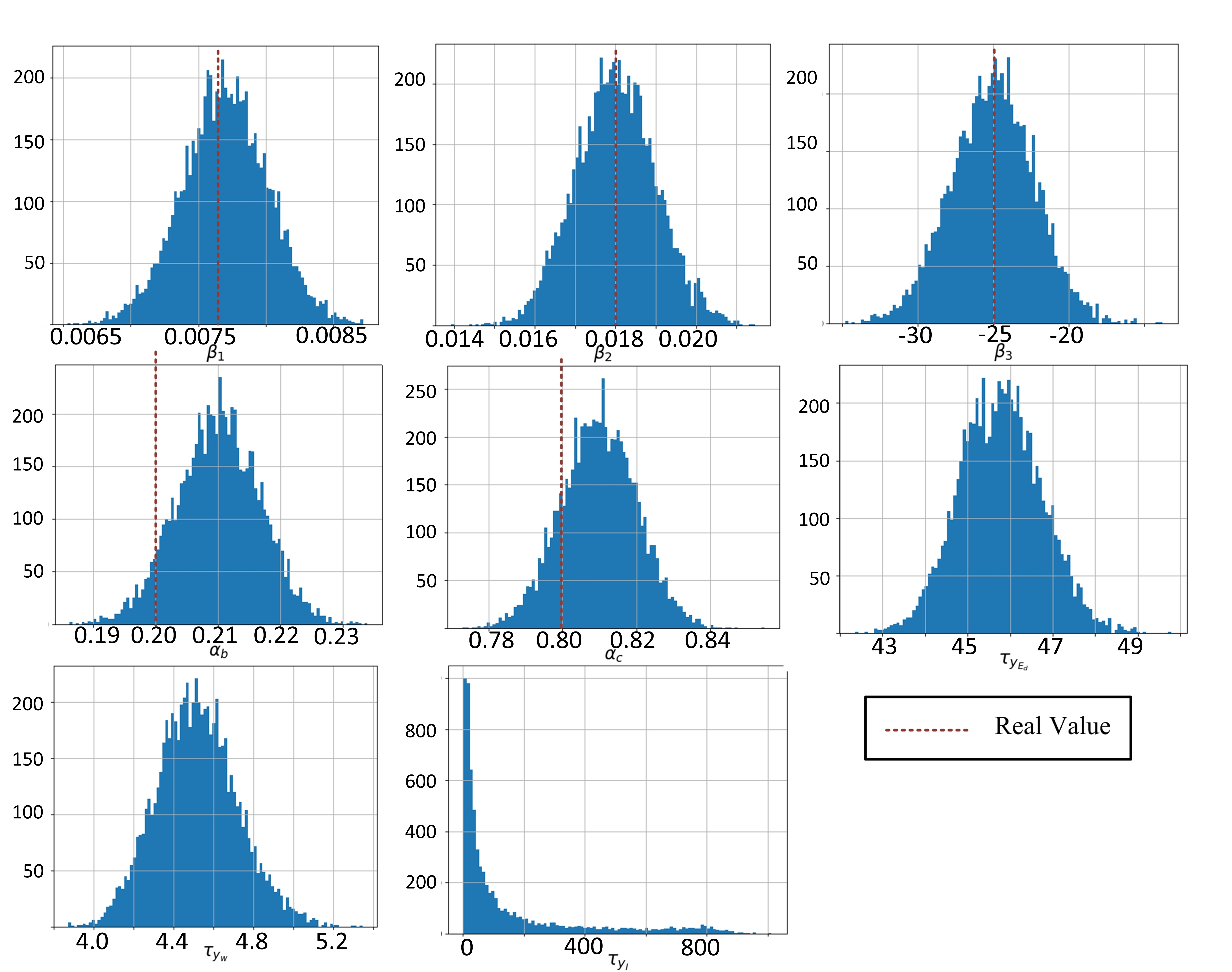 Figure 1
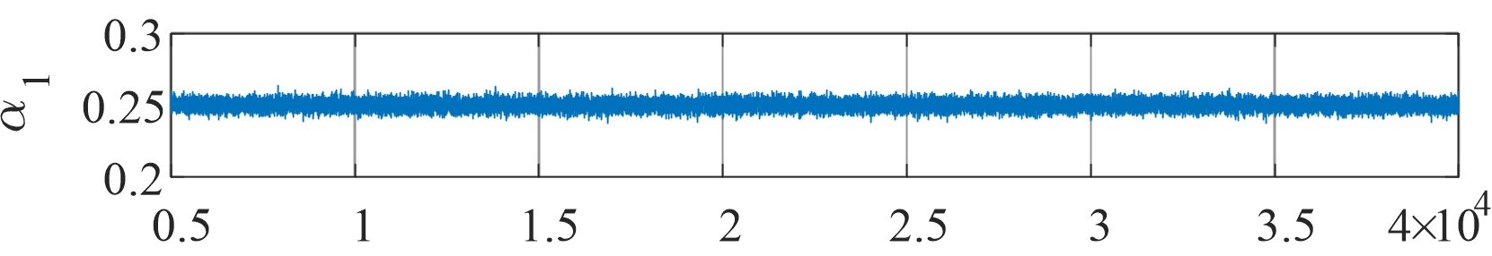 Figure 2
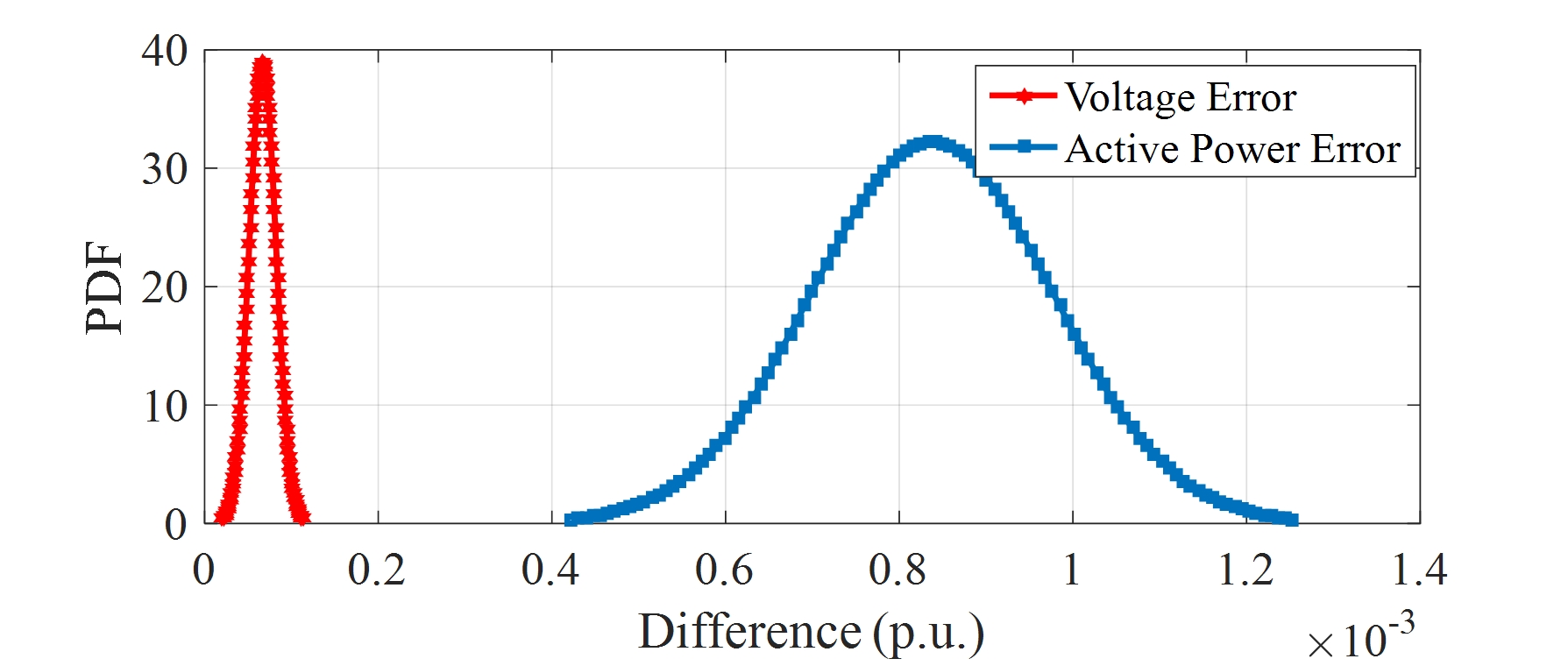 Figure 3
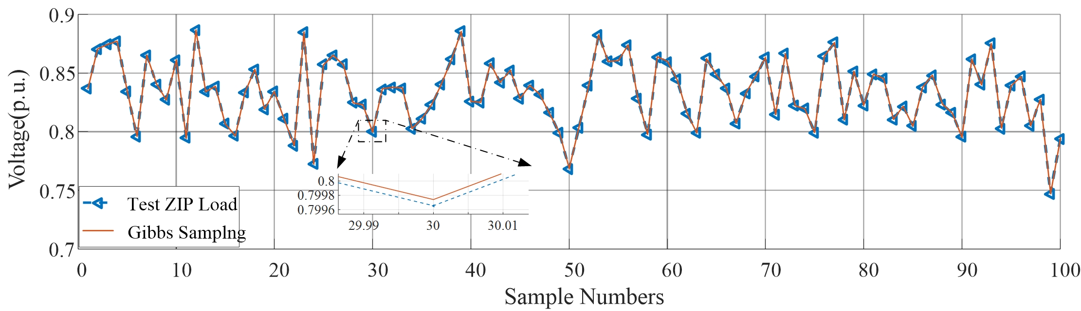 Figure 4
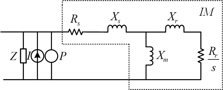 Figure 5
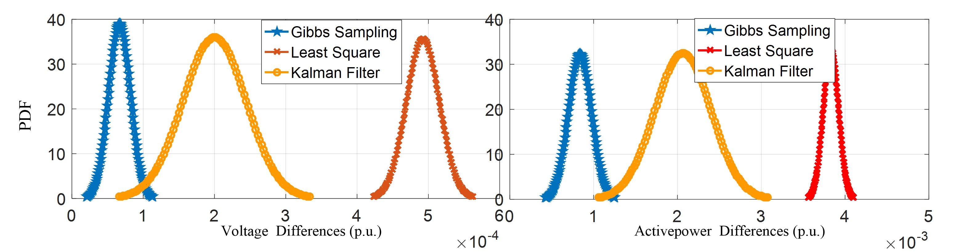 Figure 6
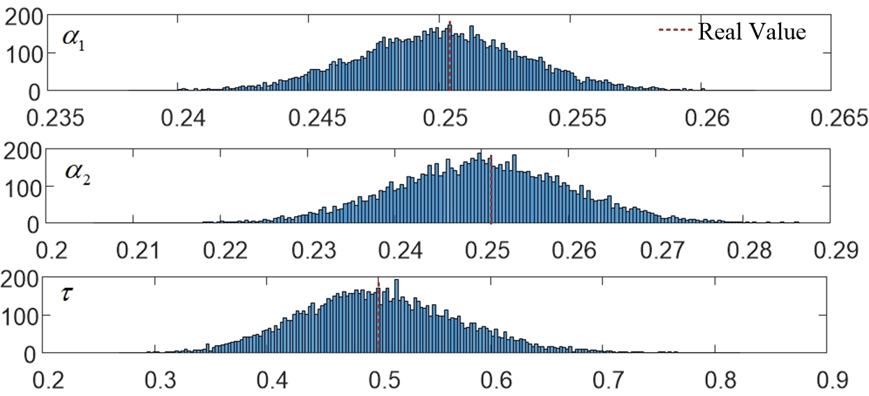 Figure 7
| Para. | Real Value | Est. Value (mean) | Error(%) |
|---|---|---|---|
| 0.0077 | 0.007683 | 0.22 | |
| 0.018 | 0.01824 | 1.33 | |
| 25 | 24.8 | 0.8 | |
| 0.20 | 0.211 | 5.5 | |
| 0.80 | 0.813 | 1.63 |
| Para. Error | GS (%) | LS(%) | KF(%) |
|---|---|---|---|
| Voltage | 0.007 | 0.062 | 0.024 |
| Active Power | 1.12 | 4.65 | 2.64 |
| Para. | GS | LS | KF | Real Value |
|---|---|---|---|---|
| 0.007683 | 0.0076 | 0.0077 | 0.0077 | |
| 0.01824 | 0.1375 | 0.0185 | 0.018 | |
| 24.8 | 18 | 34 | 25 | |
| 0.211 | 2.06 | 1.8 | 0.2 | |
| 0.813 | 4.04 | 3 | 0.8 |
Peer Reviews
No public reviews on file for this paper yet. If you reviewed it on a platform where reviews are public (OpenReview, ICLR, NeurIPS, ICML), you can paste yours below so the community can read it here.
Videos
No videos yet. Explain this paper in a talk, walkthrough, or lecture? Add one.
Taxonomy
TopicsPower System Optimization and Stability · Optimal Power Flow Distribution · Smart Grid Energy Management
Bayesian Estimation Based Parameter Estimation for Composite Load
Chang Fu
GEIRI North America, San Jose, CA, 95134, USA
College of Engineering, Wayne State University, Detroit, MI, 48201, USA
Zhe Yu
GEIRI North America, San Jose, CA, 95134, USA
Di Shi
GEIRI North America, San Jose, CA, 95134, USA
Haifeng Li
State Grid Jiangsu Electric Power Company Ltd., Nanjing, Jiangsu, 210024, China
Caisheng Wang
College of Engineering, Wayne State University, Detroit, MI, 48201, USA
Zhiwei Wang
GEIRI North America, San Jose, CA, 95134, USA
Jie Li This work is funded by SGCC Science and Technology Program under contract no. SGSDYT00FCJS1700676. State Grid US Representative Office, New York City, NY, 10017, USA
Email: [email protected]
Abstract
Accurate identification of parameters of load models is essential in power system computations, including simulation, prediction, and stability and reliability analysis. Conventional point estimation based composite load modeling approaches suffer from disturbances and noises and provide limited information of the system dynamics. In this work, a statistic (Bayesian Estimation) based distribution estimation approach is proposed for both static (ZIP) and dynamic (Induction Motor) load modeling. When dealing with multiple parameters, Gibbs sampling method is employed. In each iteration, the proposal samples each parameter while keeps others fixed. The proposed method provides a distribution estimation of load models coefficients and is robust to measurement errors.
Index Terms:
Bayesian estimation, dynamic model, Gibbs sampling, parameter estimation, static model.
I Introduction
Load models can be categorized into static and dynamic models. Conventional static models include ZIP model, exponential model, frequency dependent model, etc., and the induction motor (IM), exponential recovery load model (ERL) [1] are the major dynamic load models used in research studies recently. It is reported that a composite load under ZIP+IM model can be used with various conditions, locations and composition, and it has been widely used in industry and studied in voltage stability as well as planning, operation and control of power systems[1, 2, 3, 4].
Load models are typically identified by component and measurement based approaches in state of the art [1, 5, 6, 7, 8, 9, 10, 11, 12, 13, 14]. Component based approaches highly rely on characteristics of components and compositions of load. In [7], ZIP coefficients for widely used electrical appliances are determined by experiments, and the overall ZIP model was established with respect to the predetermined appliances. However, the computational cost is high, and the accuracy of individual consumers is greatly affected by non-electric factors such as data and weather [7, 1]. Difficulties in obtaining load composition information is another factor to be considered when implementing this type of methods.
Measurement-based approaches, such as least-squares (LS) and genetic algorithm (GA), are another mainstream for load parameter identifications. Different techniques are reported in [9, 15] to identify the parameters for composite load models. In [16], a robust time-varying load parameters identification approach is proposed by using batch-model regression in order to obtain the updated system parameters. One disadvantage of measurement based approach is the dependence on data quality. Measurement anomalies may affect the robustness of estimation in both time-varying and time-independent load models. Moreover, these approaches estimate the expected value of coefficients, which provides limited information.
Bayesian estimation (BE) [17] based composite load parameter identification approach can successfully overcome the aforementioned disadvantages in measurement and component based approaches. First, BE is a distribution estimation rather than point estimation technique, which provides the likelihood of each parameter. In this case, this method is able to provide accurate estimation of the parameters in both time constant and time-varying cases. Second, BE does not require information of load compositions, nor coefficients of appliances. Third, BE is a robust estimation method due to its statistical characteristics: measurement anomalies will not significantly affect the results if the number of samples is large enough, and the effect of measurement error is also not significant either because the distribution interval contains the real value inside the distribution with expected probabilities.
The rest of the paper is organized as follows. The problem of ZIP and IM model estimation is formulated in Section II. The Bayesian estimation technology and the detailed parameter identification method (Gibbs Sampling) is introduced in Section III. The advantage of the proposal is illustrated in Section IV by simulations. Section V draws the conclusion.
II Formulation
In this section, a composite load model consisting of ZIP and IM model is introduced [2], followed by the proposed parameter estimation method, Gibbs Sampling (GS).
A composite load with ZIP+IM model is shown in Fig. 1, in which the ZIP model describes the steady-state behavior and the IM model corresponds to the dynamic process.
II-A ZIP Model
The ZIP model describes how the power of load changes as voltage varies in the steady-state condition. The ZIP model is formulated as follows.
[TABLE]
where , , and are real and reactive power, and is voltage magnitude at the load terminal. Variables , and represent the values of the respective variables at the initial operating condition. When voltage deviates from , real and reactive power of the load is assumed to follow a quadratic model. As the real power and reactive power follow the same form of model, we will discuss only the real power as an example in the following. The reactive power follows the same procedure.
Define , , where and are the th measurements of the real power and voltage magnitude of the ZIP load. The following assumptions are made.
- •
The measurement noise follows a normal distribution, i.e., , where , and is the variance111The reasons for making this assumption are: 1) According to the law of large numbers, a normal distribution would be the best one to represent the characteristics of the noise if the number of experiment is large enough. 2) Since normal distribution is a conjugate distribution, it is easier for model parameter updating when implementing Gibbs sampling..
- •
Total number of independent and identically distributed (i.i.d.) samples were drawn, namely . Thus the likelihood
[TABLE]
where is the mean.
II-B * IM Model*
The dynamic part of load is usually represented by an IM model, which is discussed below [6].
[TABLE]
where , , , . Here is motor stator winding resistance, is motor stator leakage reactance, is motor magnetizing reactance, is rotor resistance, is rotor leakage reactance, is rotor inertia constant, is rotor speed, and are stator current in -axis and -axis, and are bus voltage in -axis and -axis, and and are stator voltage in -axis and -axis. is the initial load torque.
The parameters to be identified in an IM model are: . Typically, is assumed to be as the mechanical torque is assumed to be proportional to the square of the rotation speed of the motor [10]. Consequently B and C are both equal to 0. For simplicity, define , , , , , , , , , . Assuming that the measurement noise is i.i.d. and follows a normal distribution, we can rewrite the IM model as follows:
[TABLE]
where , , , , and .
III Bayesian Estimation in Composite Load Parameter Identification
III-A Gibbs sampling
Gibbs sampling is an extension of Monte Carlo Markov Chain method [17], which performs well when there are multiple parameters to identify. The detailed sampling algorithm is shown in Algorithm 1.
Starting with priors, Gibbs sampling estimates the posterior of one parameter while fixing others’ values as samples from previous estimated posteriors. This process repeats for all parameters in one iteration.
III-B Gibbs in ZIP Model
Start with the prior guess as follows:
[TABLE]
where the distribution of is a gamma distribution follows . It can be shown that after each iteration of Gibbs sampling, the post distributions of these three parameters remains the same form. Only the first iteration will be shown here as an example. First, samples are drawn from the prior and are initialized. After some algebraic yields:
[TABLE]
where is the posterior probability given the samples of x, y, , and , is the likelihood in (1), and is the prior estimation following (3). Taking the log form on both sides of (6) yields
[TABLE]
Taking log form helps convert the multiplications of the probabilies to summations, which can significantly simplify calculations when updating the distributions of the posteriors. For a normal distribution , the log dependence on is .
The right hand side of equation (7) can be further written as the following if the terms not related to are omitted.
[TABLE]
Define
[TABLE]
[TABLE]
yields
[TABLE]
Then sample a new from the estimated distribution as . Following the similar procedures can be derived. Define
[TABLE]
Therefore, the following can be derived:
[TABLE]
For , the posterior given new samples of and can be written as . Taking the log form of both sides of the posterior and yields
[TABLE]
Define
[TABLE]
the posterior can be obtained.
III-C Gibbs in IM models
Start with the priors as follows.
[TABLE]
The parameter identification in the IM model follows a similar procedure as the ZIP model and is omitted here for space consideration. Details can be found in [18].
IV Case Study
Simulation studies are carried out in this section for ZIP and IM models, separately. In this work, the maximum Monte Carlo runs is set to 40000 and the burn-in length is chosen as 5000 [17].
IV-A ZIP Model Identification
The 33-bus test feeder [19] is used to generate the testing data. A detailed description of the test system can be found in [18]. Load at bus 18 is replaced by a ZIP model. Randomness is added to loads at other buses by multiplying a random factor drawing from a uniform distribution following . The random load is stated as , where is the original load in the 33-bus test feeder, indicates the node number, and is the weighted load at the corresponding node after multiplying a random weight. The changes at each load in every experiment simulates the disturbances and uncertainties in the system, which significantly impact the voltage and power at the bus of interest.
The ZIP factors of the load at node 18 were assigned as , , . Power flow converges in each iteration with different , and the corresponding voltage is recorded. The measurement noise follows , which means a 10% measurement error.
By implementing the proposed GS method, the coefficients of the ZIP model are estimated as shown in Fig. 2.
Different from other estimation approaches, the GS approach can generate a distribution which describes the probability of the real value falling into a certain range. As shown in Fig. 2, the mean values of the distributions of and are 0.25 and 0.249, respectively, and .
Figs. 3 and 4 show the voltage and voltage/real power differences, respectively, using the estimated and real model in 100 i.i.d. experiments. The randomness comes from the factors multiplied to loads at other buses. The dash line with triangle in Fig. 3 indicates the voltage at bus 18 using the real ZIP coefficients, and the solid line is the voltage measured at the same bus using estimated coefficients. The comparison shown in Fig. 4 is the distributions of voltage and active power differences, and . It can be seen that the differences are in the range of 10*-4* and 10*-3*, respectively. Fig. 5 shows the burn-in process observed. It shows that the process is very fast, and there is no significant burn-in process that can be observed from this figure.
IV-B IM model Identification
The estimation of the parameters in the IM model follows the same procedure. A dynamic model is built in Matlab/Simulink to generate the data that is used in (2). The sampling results are shown in Fig. 6 and compared with the real data in Table I. According to Table I, the estimation error are less than 6% with 5% measurements error. It is worth to mention that estimation of parameters highly relies on the prior distributions. A good prior can significantly increase the estimation accuracy and shorten the burn-in period.
IV-C Benchmarks
The ZIP and IM model parameters derived by the proposed GS method are compared with least square (LS) [20] and Kalman Filter (KF) methods [21] with 10% noise. The “fit” function in Matlab was used to derive the coefficients in LS. The parameter tuning in KF was introduced in [21], and these parameters were directly used in this study. The comparison results of the voltage and active power using GS, LS, and KF in ZIP model are shown in Fig 7. The average absolute mean of voltage and active power errors in p.u. are listed in Table II. According to Fig 7, it is obvious that GS approach has the best performance, while KF method only falls slightly behind. In contrast, LS gives the largest error among all three approaches when there is large measurement error. However, KF only works well with time-invariant parameters estimation [22]. In practice, the ZIP component varies with time due to stochastic consumer behaviors.
The parameters estimation comparisons in the IM model are listed in Table III. The estimation errors from GS are the smallest. The performance of KF is worse than itself in the ZIP model, but still better than the LS method.
V Conclusion
In this paper, a novel Bayesian estimation based load model parameter identification method is proposed. The proposed method can accurately identify the parameter distributions for both ZIP and IM models. Compared with other measurement based algorithms, the proposed method provides a distribution estimation and is robust to measurement errors. The accuracy and robustness of the proposed method compared with conventional load modeling method are also demonstrated by numerical experiments. The identified distributions can be further used in load prediction, stability and reliability analysis, as well as other related areas. Further study may include how to estimate the ZIP and IM model jointly and extending the process in an online manner.
The reference list from the paper itself. Each links out to its DOI / PubMed record.
- 1[1] A. Arif, Z. Wang, J. Wang, B. Mather, H. Bashualdo, and D. Zhao, “Load modeling – a review,” IEEE Transactions on Smart Grid , pp. 1–1, 2017.
- 2[2] P. Kundur, N. J. Balu, and M. G. Lauby, Power system stability and control . Mc Graw-hill New York, 1994, vol. 7.
- 3[3] J.-K. Kim, K. An, J. Ma, J. Shin, K.-B. Song, J.-D. Park, J.-W. Park, and K. Hur, “Fast and reliable estimation of composite load model parameters using analytical similarity of parameter sensitivity,” IEEE Transactions on Power Systems , vol. 31, no. 1, pp. 663–671, 2016.
- 4[4] S. Alyami, C. Wang, and C. Fu, “Development of autonomous schedules of controllable loads for cost reduction and pv accommodation in residential distribution networks,” in Electrical Power and Energy Conference (EPEC), 2015 IEEE . IEEE, 2015, pp. 81–86.
- 5[5] J. V. Milanovic, K. Yamashita, S. M. Villanueva, S. Djokic, and L. M. Korunović, “International industry practice on power system load modeling,” IEEE Transactions on Power Systems , vol. 28, no. 3, pp. 3038–3046, Aug 2013.
- 6[6] H. Renmu, M. Jin, and D. J. Hill, “Composite load modeling via measurement approach,” IEEE Transactions on Power Systems , vol. 21, no. 2, pp. 663–672, May 2006.
- 7[7] Z. Yu, L. Mc Laughlin, L. Jia, M. C. Murphy-Hoye, A. Pratt, and L. Tong, “Modeling and stochastic control for home energy management,” IEEE Transactions on Smart Grid , vol. 4, no. 4, pp. 2244–2255, 2012.
- 8[8] J. V. Milanović and S. M. Zali, “Validation of equivalent dynamic model of active distribution network cell,” IEEE Transactions on Power Systems , vol. 28, no. 3, pp. 2101–2110, Aug 2013.