Bayesian optimization for tuning and selecting hybrid-density functionals
Rodrigo A. Vargas-Hern\'andez

TL;DR
This paper demonstrates that Bayesian optimization can efficiently tune parameters and select the best hybrid-density functional models, significantly reducing computational effort compared to traditional grid search methods.
Contribution
It introduces the application of Bayesian optimization for tuning and selecting density functional models, including joint optimization of parameters and functional form, in material science.
Findings
BO requires approximately 55 evaluations for optimal parameter tuning.
BO can identify the most suitable exchange-correlation functional without prior info.
Joint optimization with BO improves accuracy in predicting atomization energies.
Abstract
The accuracy of some density functional (DF) models, widely used in material science, depends on empirical or free parameters which are commonly tuned using reference physical properties. The optimal value of the free parameters is regularly found using grid search algorithms, which computational complexity scales with the number of points in the grid. In this report, we illustrate that Bayesian optimization (BO), a sample-efficient machine learning algorithm, can efficiently calibrate different density functional models, e.g., hybrid-exchange-correlation and range-separated density functionals. We present that, BO can optimize the free parameters of hybrid-exchange-correlation functionals, with approximately 55 evaluations of the root-mean-square or mean-absolute error functions of the atomization energies and the bond length of the Gaussian-1 (G1) database. We also illustrate that BO…
Click any figure to enlarge with its caption.
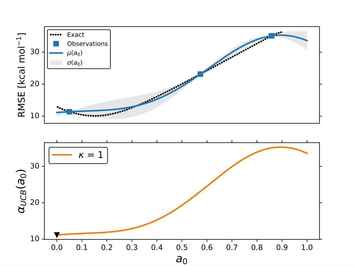 Figure 1
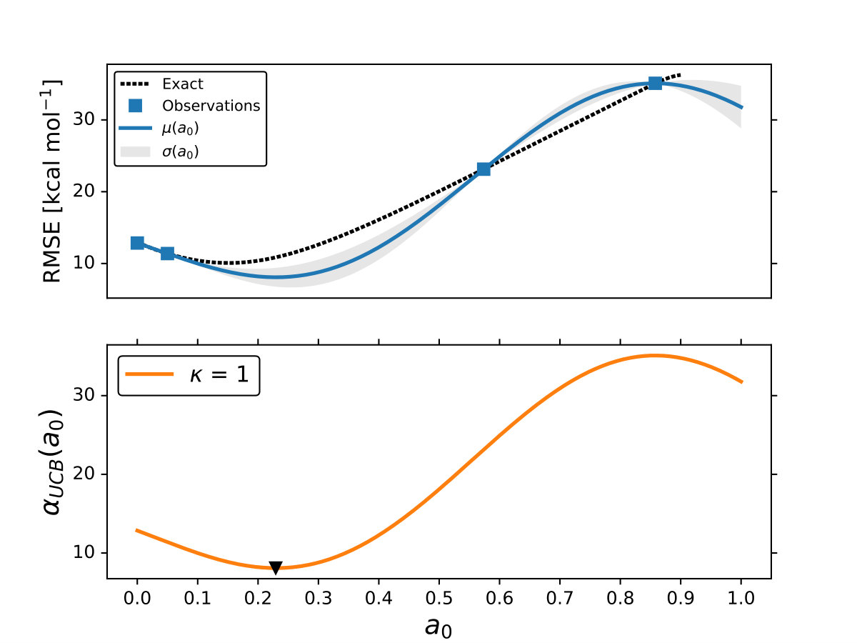 Figure 2
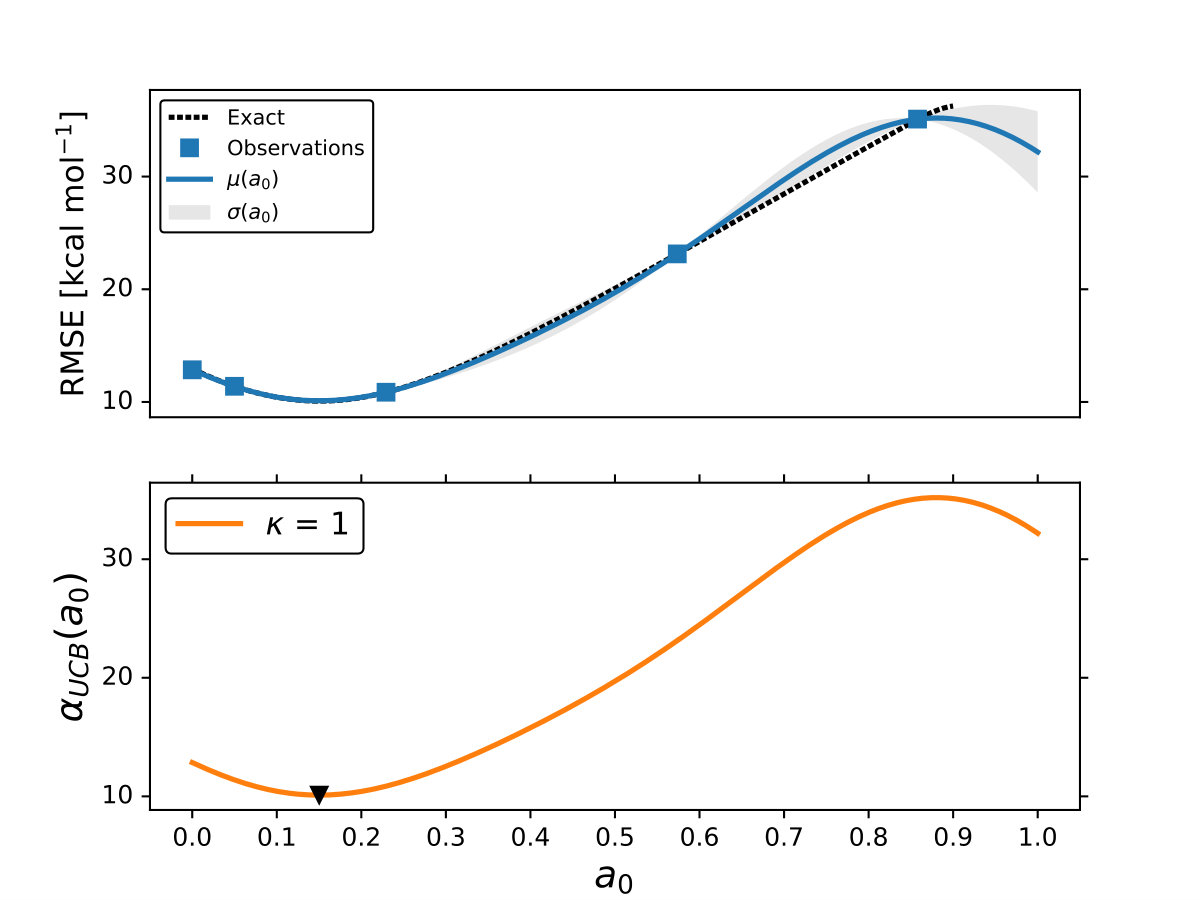 Figure 3
 Figure 4
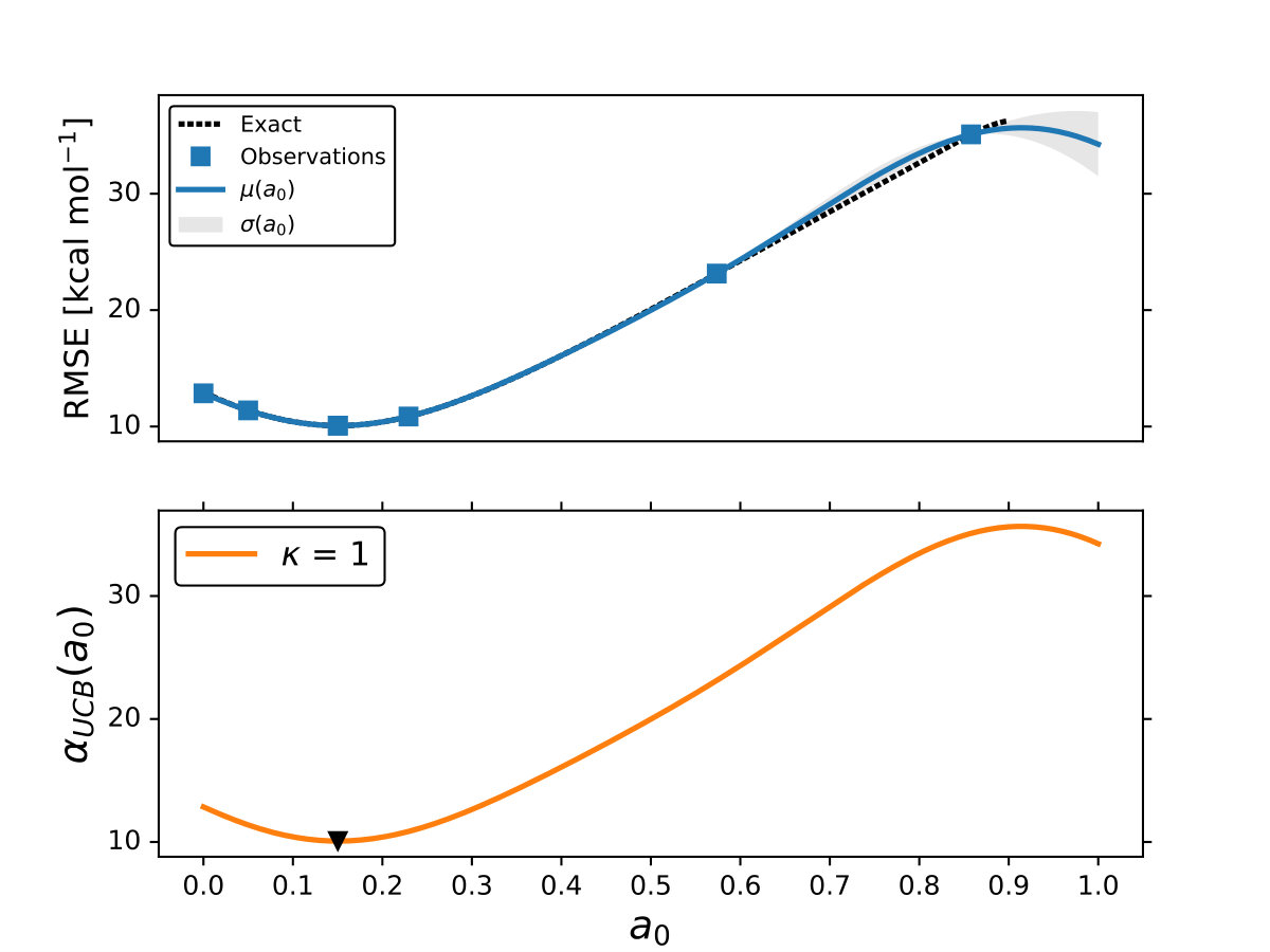 Figure 5
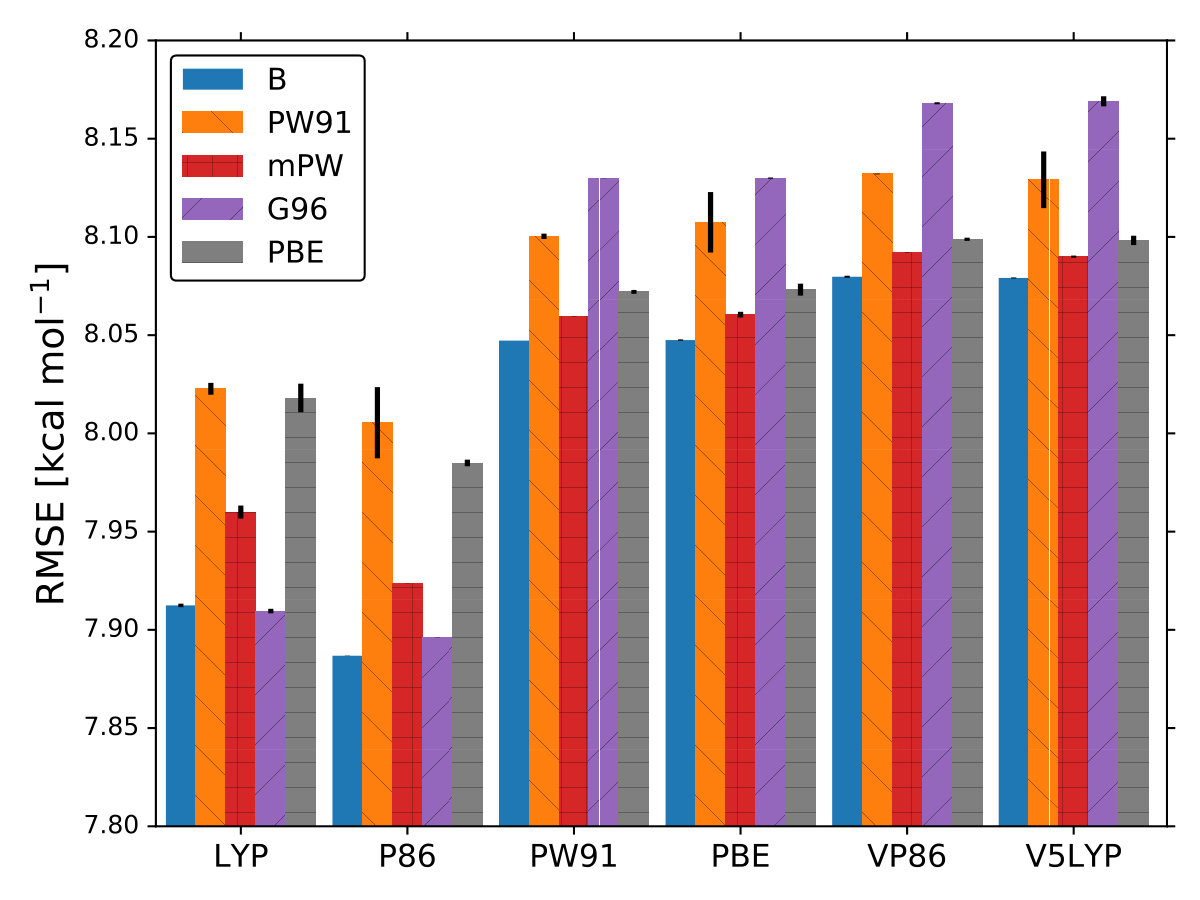 Figure 1
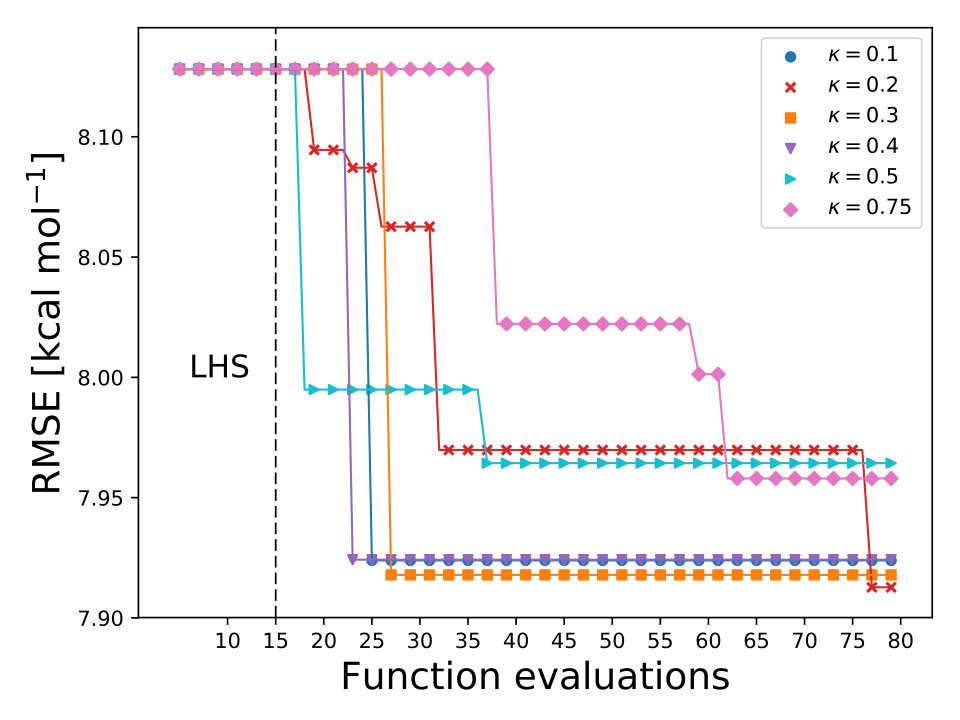 Figure 2
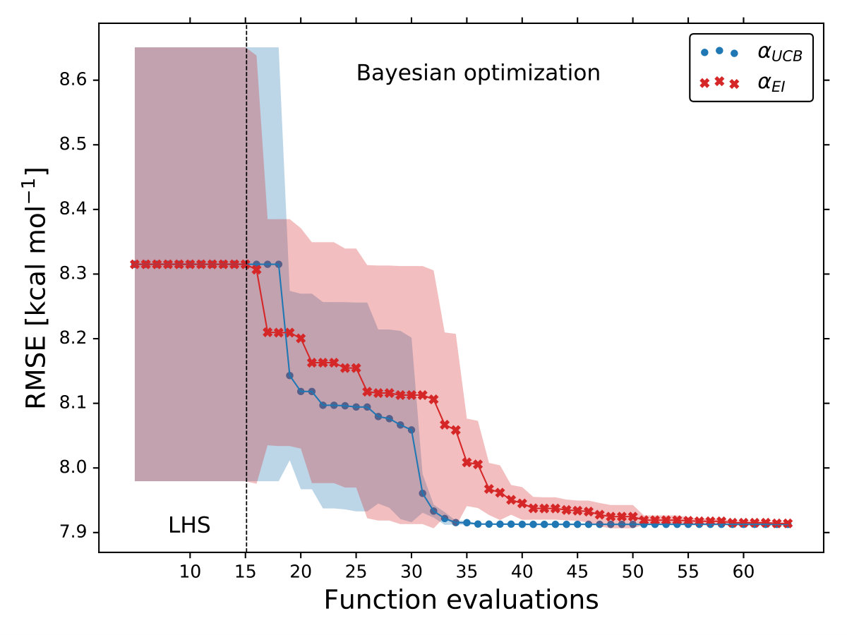 Figure 2
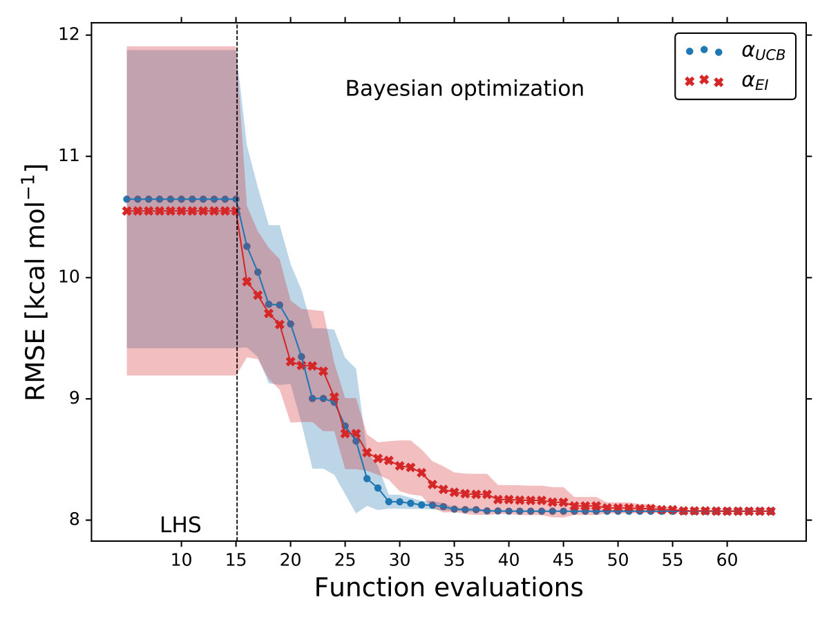 Figure 2
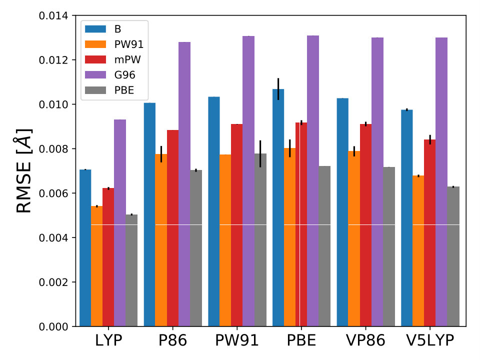 Figure 3
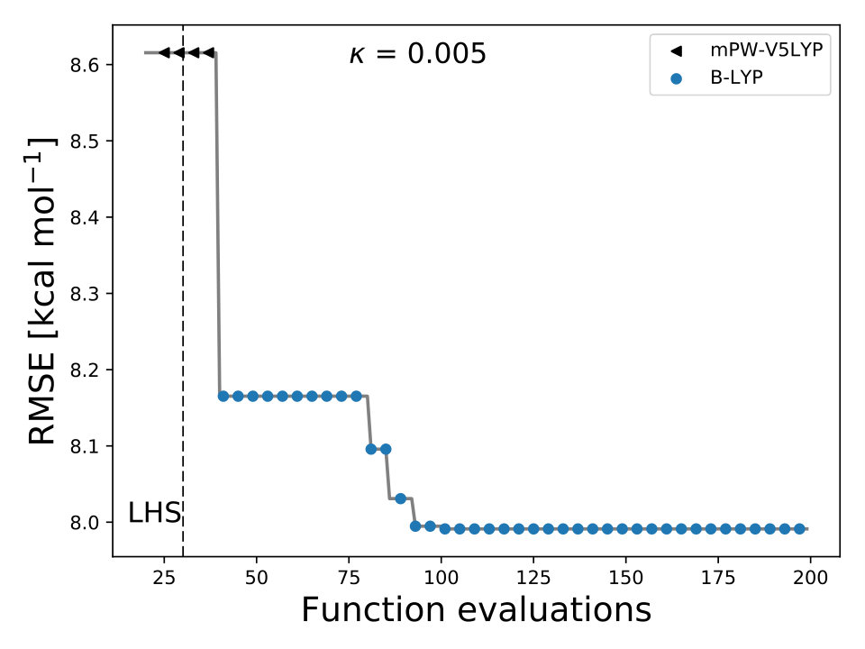 Figure 3
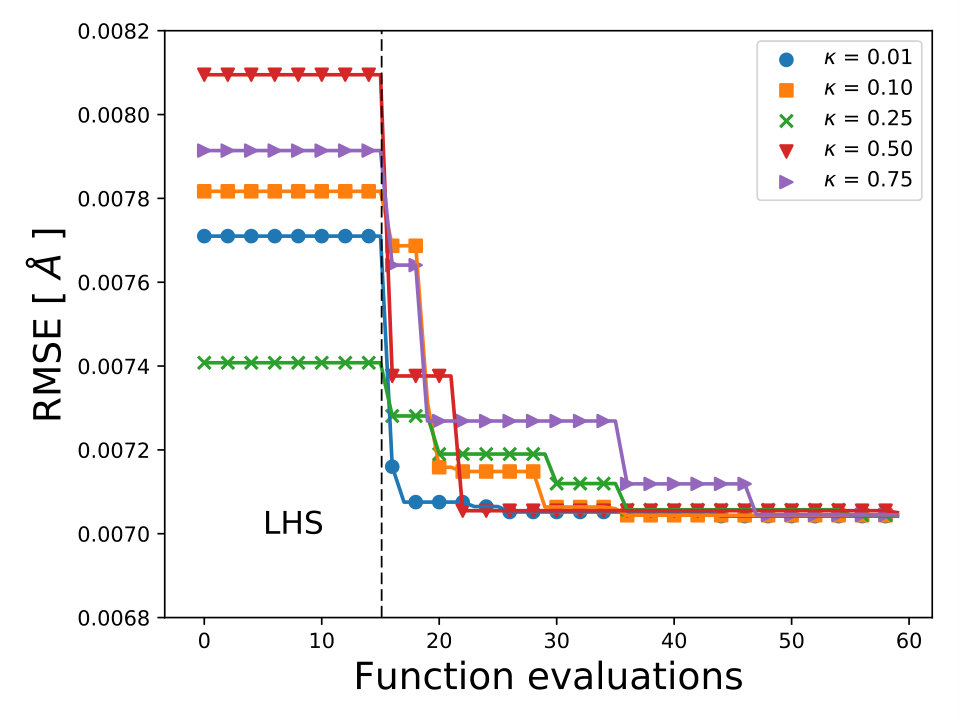 Figure 3
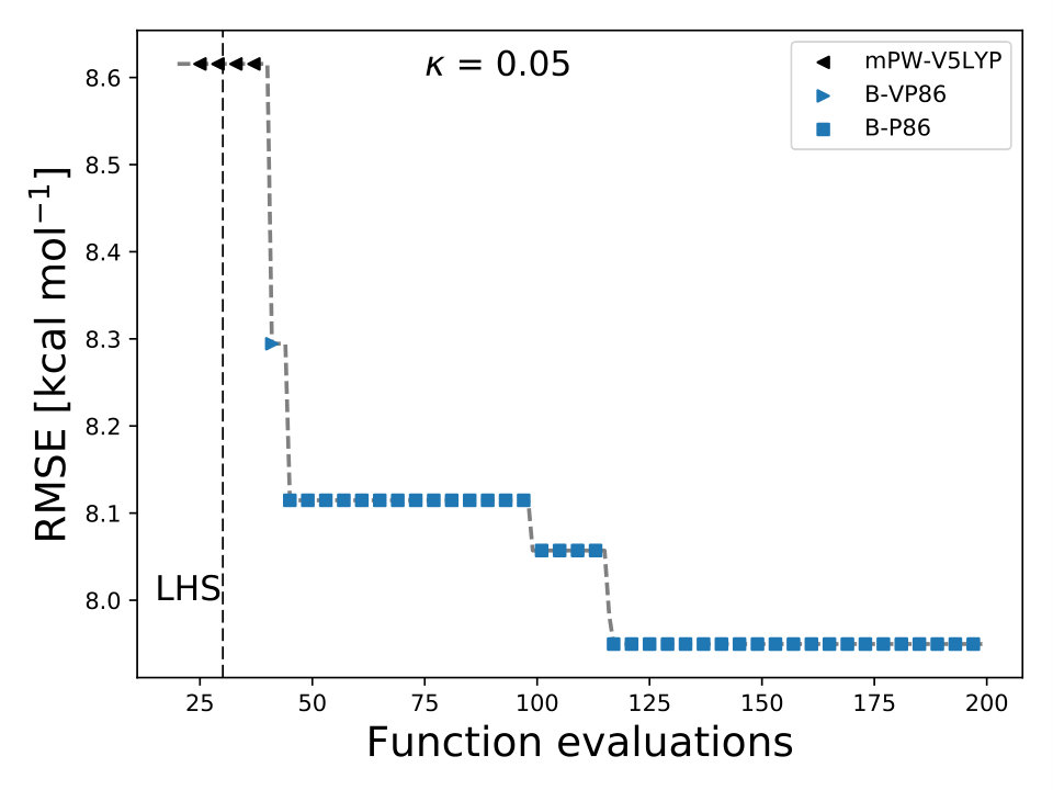 Figure 3
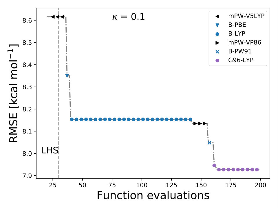 Figure 3
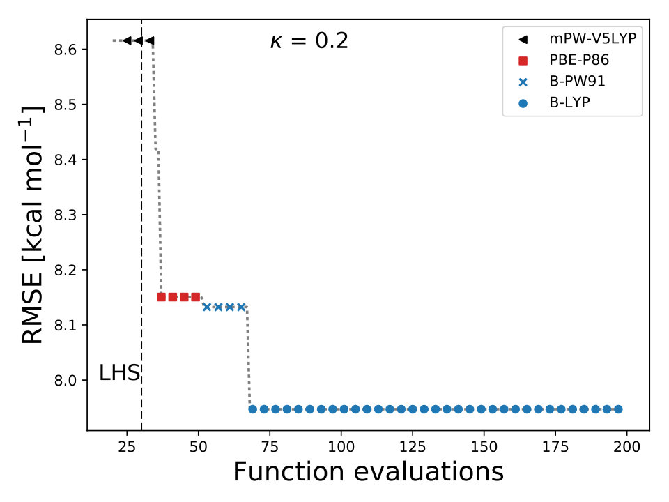 Figure 3
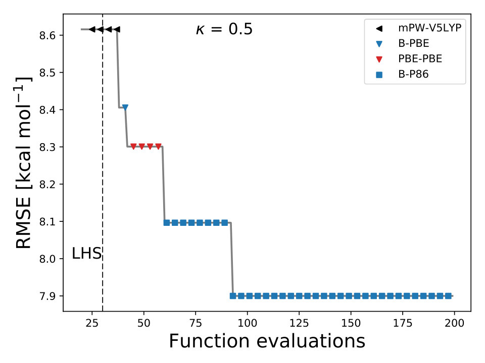 Figure 3
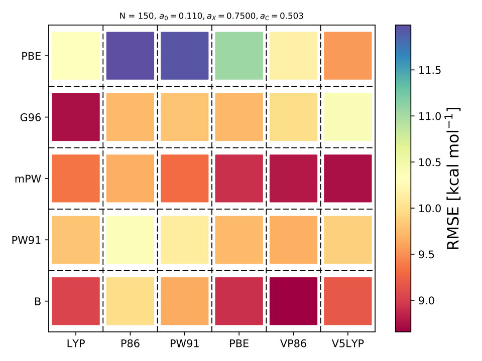 Figure 4
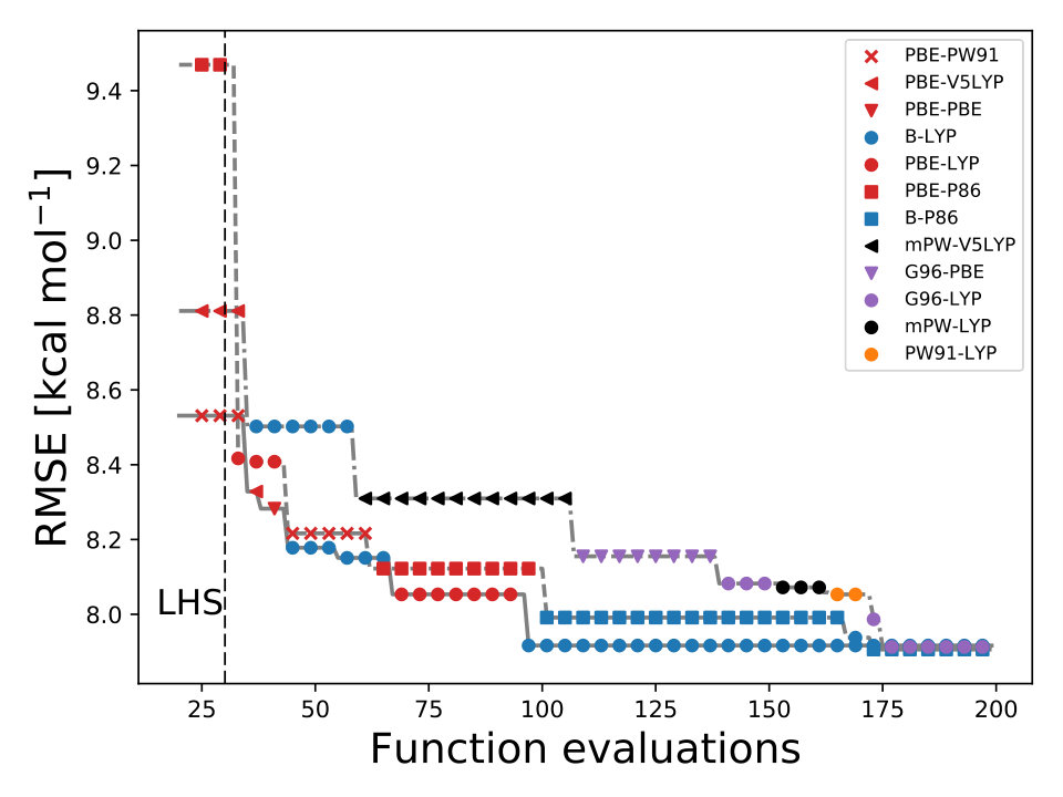 Figure 4
| basis set | ||||
|---|---|---|---|---|
| PBE0111Refs. acm_theory ; PBE0_1 | – | 0.25 | 0.75 | 1.0 |
| B3LYP222Refs. B_acm3_0 ; B3LYP ; B3LYP_2 | – | 0.20 | 0.72 | 0.81 |
| PBE-PBE333Tables III SM and VIII SM | 6-31G() | 0.1028 | 0.8708 | 0.0292 |
| 6-311G() | 0.1173 | 0.8742 | 0.1967 | |
| 6-311++G() | 0.1293 | 0.8855 | 0.3537 | |
| B-LYP333Tables III SM and VIII SM | 6-31G() | 0.1100 | 0.8293 | 0.0201 |
| 6-311G() | 0.1500 | 0.7658 | 0.3748 | |
| 6-311++G() | 0.1924 | 0.6962 | 0.7080 |
| Molecule | PBE01116-311++G() | B3LYP1116-311++G() | PBE-PBE1116-311++G(),333 = 0.1173, = 0.8742, = 0.1967. | B-LYP1116-311++G(),444 = 0.1293, = 0.8855, = 0.3537. | PBE-PBE2226-311++G(),555 = 0.1500, = 0.7658, = 0.3748. | B-LYP2226-311++G(),666 = 0.1924, = 0.6962, = 0.7080. | Exp.777From Refs. G1 ; G1_1 ; G1_2 |
| H2 | 98.00 | 103.84 | 107.51 | 107.06 | 105.59 | 104.26 | 103.5 |
| LiH | 50.72 | 56.39 | 59.52 | 59.06 | 57.84 | 56.76 | 56.0 |
| BeH | 52.90 | 55.05 | 56.26 | 56.56 | 55.63 | 55.25 | 46.9 |
| CH | 79.00 | 81.53 | 82.38 | 82.08 | 82.18 | 81.31 | 79.9 |
| CH2(trip.) | 179.30 | 177.95 | 179.90 | 178.92 | 180.12 | 178.51 | 179.6 |
| CH2(sing.) | 133.40 | 138.15 | 137.74 | 137.74 | 139.02 | 138.62 | 170.6 |
| CH3 | 289.75 | 291.42 | 294.26 | 293.56 | 293.43 | 292.28 | 289.2 |
| CH4 | 389.68 | 393.03 | 397.46 | 396.90 | 395.13 | 394.39 | 392.5 |
| NH | 80.63 | 83.53 | 83.27 | 83.08 | 83.81 | 82.96 | 79.0 |
| NH2 | 171.25 | 176.27 | 175.35 | 175.31 | 176.16 | 175.33 | 170.0 |
| NH3 | 273.60 | 279.80 | 278.64 | 278.99 | 279.91 | 279.76 | 276.7 |
| OH | 100.69 | 103.30 | 101.35 | 101.63 | 103.01 | 102.84 | 101.3 |
| OH2 | 214.16 | 218.23 | 214.05 | 214.78 | 217.38 | 217.74 | 219.3 |
| FH | 131.65 | 134.11 | 129.68 | 130.31 | 133.46 | 133.88 | 135.2 |
| Li2 | 19.06 | 20.48 | 22.44 | 20.78 | 21.84 | 20.55 | 24.0 |
| LiF | 130.91 | 135.84 | 134.65 | 135.00 | 134.99 | 135.04 | 137.6 |
| HCCH | 387.55 | 386.51 | 387.38 | 386.98 | 387.73 | 387.59 | 388.9 |
| H2CCH2 | 532.05 | 531.64 | 534.17 | 533.58 | 533.41 | 533.25 | 531.9 |
| H3CCH3 | 665.42 | 665.12 | 670.39 | 669.57 | 667.58 | 667.39 | 666.3 |
| CN | 176.13 | 176.68 | 178.19 | 177.13 | 178.30 | 176.48 | 176.6 |
| HCN | 301.45 | 303.66 | 304.24 | 304.17 | 304.09 | 303.73 | 301.8 |
| CO | 253.36 | 253.11 | 252.53 | 252.87 | 252.09 | 252.59 | 256.2 |
| HCO | 273.49 | 273.32 | 272.73 | 272.56 | 273.02 | 273.07 | 270.3 |
| H2CO | 356.92 | 358.00 | 358.08 | 358.09 | 358.23 | 358.32 | 357.2 |
| H3COH | 478.70 | 480.54 | 479.37 | 479.72 | 480.11 | 481.04 | 480.8 |
| N2 | 221.97 | 226.12 | 225.23 | 225.41 | 225.03 | 224.45 | 225.1 |
| H2NNH2 | 402.04 | 408.60 | 407.09 | 407.67 | 408.01 | 408.49 | 405.4 |
| NO | 151.24 | 152.96 | 152.45 | 152.32 | 151.97 | 151.46 | 150.1 |
| O2 | 122.36 | 121.68 | 121.73 | 121.19 | 120.03 | 119.74 | 118.0 |
| HOOH | 247.09 | 251.18 | 248.88 | 249.44 | 249.40 | 250.06 | 252.3 |
| F2 | 32.63 | 34.76 | 35.99 | 35.20 | 33.32 | 32.87 | 36.9 |
| CO2 | 386.40 | 382.39 | 380.60 | 381.04 | 380.72 | 381.61 | 381.9 |
| RMSE | 7.378 | 6.350 | 6.763 | 6.670 | 6.326 | 6.263 | |
| MAE | 3.845 | 3.067 | 3.853 | 3.711 | 3.405 | 3.094 |
| Molecule | PBE0111From Ref. acm_theory | B3LYP | B-LYP222 = 0.1467, = 0.6323 , = 0.001.,444Optimized with BO and with = 0.1. | PBE-PBE333 = 0.1979, = 0.7957 , = 0.001.,444Optimized with BO and with = 0.1. | Exp.555From Refs. G1 ; G1_1 ; G1_2 |
|---|---|---|---|---|---|
| H2 | 0.745 | 0.744 | 0.741 | 0.738 | 0.742 |
| LiH | 1.597 | 1.592 | 1.588 | 1.587 | 1.595 |
| BeH | 1.347 | 1.344 | 1.339 | 1.338 | 1.343 |
| CH | 1.126 | 1.128 | 1.125 | 1.123 | 1.120 |
| NH | 1.040 | 1.044 | 1.042 | 1.040 | 1.045 |
| OH | 0.971 | 0.975 | 0.974 | 0.973 | 0.971 |
| FH | 0.916 | 0.920 | 0.919 | 0.918 | 0.917 |
| Li2 | 2.705 | 2.705 | 2.694 | 2.694 | 2.670 |
| LiF | 1.559 | 1.560 | 1.565 | 1.566 | 1.564 |
| CN | 1.163 | 1.166 | 1.166 | 1.166 | 1.172 |
| CO | 1.125 | 1.127 | 1.127 | 1.127 | 1.128 |
| N2 | 1.093 | 1.095 | 1.096 | 1.096 | 1.098 |
| NO | 1.143 | 1.148 | 1.149 | 1.149 | 1.151 |
| O2 | 1.194 | 1.206 | 1.207 | 1.208 | 1.207 |
| F2 | 1.401 | 1.408 | 1.412 | 1.416 | 1.412 |
| RMSE | 1.1E-2 | 9.68E-3 | 7.04E-3 | 7.21E-3 | |
| MAE | 7.33E-3 | 5.30E-3 | 4.19E-3 | 4.67E-3 |
Peer Reviews
No public reviews on file for this paper yet. If you reviewed it on a platform where reviews are public (OpenReview, ICLR, NeurIPS, ICML), you can paste yours below so the community can read it here.
Videos
No videos yet. Explain this paper in a talk, walkthrough, or lecture? Add one.
Current Address: ]Chemical Physics Theory Group, Department of Chemistry, University of Toronto, Toronto, ON Canada M5S 3H6.
Bayesian optimization for tuning and selecting hybrid-density functionals
R. A. Vargas–Hernández
Department of Chemistry, University of British Columbia, Vancouver, British Columbia, Canada, V6T 1Z1.
[
Abstract
The accuracy of some density functional (DF) models, widely used in material science, depends on empirical or free parameters which are commonly tuned using reference physical properties. The optimal value of the free parameters is regularly found using grid search algorithms, which computational complexity scales with the number of points in the grid. In this report, we illustrate that Bayesian optimization (BO), a sample-efficient machine learning algorithm, can efficiently calibrate different density functional models, e.g., hybrid-exchange-correlation and range-separated density functionals. We present that, BO can optimize the free parameters of hybrid-exchange-correlation functionals, with approximately 55 evaluations of the root-mean-square or mean-absolute error functions of the atomization energies and the bond length of the Gaussian-1 (G1) database. We also illustrate that BO can identify, without any prior information, the most appropriate exchange-correlation functional by navigating through the space of density functional models. We optimize and select the free parameters and the exchange-correlation functional form jointly by also minimizing the root-mean-square error function with respect to the atomization energies of the G1 database using BO.
pacs:
Valid PACS appear here
Introduction. Computational models based on density functional theory (DFT) is the workhorse of quantum mechanical simulations for predicting structures, energetics, and other physical properties across different fields. While DFT is in principle an exact theory, most of density functional (DF) models are not considered ab initio methods as they contain empirical parameters dftbook . Over the last decades a great variety of DF models have been proposed dft_revmodphys ; dft_HGordon_benchmark . With the large variety of DF models it is critical to understand which model better predicts the physical properties of the system of interest. This has lead to a large number of benchmark studies where different DF models are compared dft_HGordon_benchmark ; DFT_benchmark0 ; DFT_benchmark1 ; DFT_benchmark2 . However, due to the wide range of applications of DF models in material science, an automated model selection method is necessary for an accurate prediction of molecular properties DFT_to_ML .
The selection of physical models can be formulated as an optimization problem where the free parameters of a model, denoted as , are tuned to best reproduce the physical properties ML_optbook ; ML_opt . Commonly a loss or cost function, , is used to determine the relation between the free parameters and the accuracy of the models. The minimizer of is the value of the free parameters for the most accurate model,
[TABLE]
Any function can be minimized using gradient-based methods ML_opt ; ML_optbook by computing the change of with respect to its parameters. For DF models, the gradient of with respect to any of the free parameters may not have a simple analytical form since it also depends on the physical property, denoted as , chosen to evaluate the accuracy of the model, . Because of the complexity to compute the gradient of with respect the , grid search methods are the common approach to optimize DF dftbook ; B_acm3_0 ; B_acm3_1 ; OptB3LYP . In this letter we present a scheme based on a machine learning (ML) algorithm to efficiently screen different DF models.
ML algorithms have been demonstrated to be powerful numerical tools to simulate many-body physics vonLilienfeld ; vonLilienfeld_2 ; Aspuru_NNmolecules ; Wang_prb ; Carleo_science ; Carrasquilla_natphys ; ravh_prl ; Aspuru_NNmolecules_2 , e.g., reducing the computational complexity in DF calculations by bypassing the Kohn-Sham equations KE_DFT ; ML_DFT ; ML_DFT_2 . Likewise, Bayesian ML models have been used to study quantum systems RK_bayesML ; for instance, the optimization for producing Bose-Einstein condensates GPBEC , simulate chemical reactions Reiher_chemrxn_error ; Reiher_chemrxn_error2 and controlling a robot to do chemical synthesis phoenics ; chemos , both using a probabilistic regression model. Additionally, the error of DF models has also been estimated using Bayesian statistics BEE_PRL ; BEE_PRB ; Bayes_DFT_0 ; Bayes_DFT_1 ; Walter_BEE ; mBEEF ; Bayes_DFT_water .
One of the most important results of ML are the optimization methods designed to minimize complex functions to train and select ML models ML_optbook ; ML_opt . Bayesian optimization (BO) is one of the most common ML algorithms used to minimize functions whose gradients can not be computed BO_Adams ; BO_Freitas . In the field of molecular physics, BO was recently used to generate low-energy molecular conformers BO_PES ; BO_geo , and to build global potential energy surfaces for reactive molecular systems using feedback from quantum scattering calculations ravh_njp . BO has also been applied to efficiently screen for chemical compounds BO_mat ; BO_dft_calc ; BO_phonono_transport , and to minimize the energy function for the Ising model BO_ising . In this contribution we demonstrate that the parameters of a DF model can be efficiently tuned using BO. We consider two cases, i) the search for the optimal values of the free parameters DF, e.g., hybrid exchange-correlation (XC) and range-separated functionals, and ii) the search for the most accurate XC functional form. The value of the methodology presented here is clear since automation to improve DF models is one of the most important goals in computational physics, chemistry and material science.
Method. Bayesian optimization is a sequential search algorithm designed to find the global minimizer (or maximizer) of an unknown non-analytic or oracle function, Eq. 1. BO requires two components: a model that approximates and an acquisition function, BO_Adams ; BO_Freitas . Here we use Gaussian process (GP) models as the probabilistic model to approximate gpbook . GP model is a non-parametric regression model , whose function values are jointly Gaussian distributed. The prediction of a new point using GP models is carried out by computing the conditional distribution of given training data, denoted as . The conditional distribution has a closed form characterized by its mean, , and standard deviation, ,
[TABLE]
where is the design or covariance matrix with matrix elements , where is the kernel function. For this work we used the radial basis function (RBF) kernel,
[TABLE]
where is a diagonal matrix that has different length-scale parameter, , for each dimension of . All are described as . The parameters of the kernel function are optimized by maximizing the log marginal likelihood,
[TABLE]
where is the total number of points in and is the determinant of the design matrix. For more details on GP models, see Refs. gpbook ; sm_gp .
The goal of BO is to reduce the computational complexity of minimizing , by iteratively minimizing , which is less computationally demanding BO_Adams ; BO_Freitas . In BO, the acquisition function quantifies the informational gain if were evaluated at a new point, . Here, we only considered two acquisition functions: the expected improvement (EI),
[TABLE]
where , is the normal cumulative distribution and is the normal probability distribution. is the minimum value observed in the training data, . Secondly, we considered the upper confidence bound (UCB),
[TABLE]
where is the exploration-exploitation constant. For all the results presented in this work we set . For both acquisition functions, and are the mean and the standard deviation from a GP model, Eqs. (2) and (3). By sequentially minimizing the acquisition function and evaluating in the proposed points, BO finds the minimum/maximum of a non-analytic function, such as SM_PBE0 .
The most common DF methods are the hybrid-density functionals, introduced by Becke B_acm3_0 ; B_acm3_1 , which combine local and non-local treatments of exchange (X) and correlation (C) with the Hartree-Fock (HF) exchange,
[TABLE]
where , , and are adjustable parameters, and are the generalized gradient approximation (GGA) exchange and correlation functionals, and is the local spin density (LSD) part. Hybrid functionals of the form of Eq. 8 are usually referred to collectively as ACM3 B_acm3_0 ; B_acm3_1 ; acm_theory . In the following section we present how BO can optimize the values of , , and , and select the most accurate par of XC functional given a benchmark set of physical properties, .
Results. The loss function we considered for the optimization of all the different DF models is the root mean square error (RMSE) function,
[TABLE]
where is the atomization energy of the Gaussian-1 (G1) database G1 ; G1_1 ; G1_2 and is the atomization energy predicted with a DF model . are the free parameters of and is the total number of physical properties used in the error function, . All the DF calculations are performed with the Gaussian 09 suite G09 , and the molecular geometries used in the DF calculations were optimized with MP2/6-31G().
First we optimized the free parameter of PBE0 where, and acm_theory0 ; acm_theory ; PBE0_1 using BO with the UCB acquisition function with , and the basis set 6-31G() . With only 6 total evaluations of , BO found that the lowest RMSE is when ; kcal mol*-1*. The value of the RMSE predicted with the original PBE0 acm_theory ; PBE0_1 , , is kcal mol*-1* SM_PBE0 .
We also considered the jointly optimization of the , , and for 30 different XC functionals using BO; combination of 5 different X functionals exchange , , and 6 different C functionals correlation .
For each XC functional we carried out 5 different optimizations with different 15 initial points, where is the dimensionality of , . These points were sampled using the latin hyper cube sampling (LHS) algorithm LHS to avoid sampling multiple points close to each other. For all calculations we used 6-31G() and the molecular geometries were optimized with MP2/6-31G(). The lowest RMSE found by BO for each XC functional is displayed in Fig. 1. For each optimization, the maximum number of iterations allowed was 70 total points including the LHS points. The optimized coefficients for all 30 XC functionals are reported in Table III SM.
As it is mentioned above, the goal of BO is to circumvent the optimization problem of to a sequential optimization of , which is a less computational demanding task. In the case of the UCB function, the exploration-exploitation constant allows us to probe the space of without being trapped in a possible local minimum. In the limit where , the maximum of is where the GP model is less certain, allowing us to explore the space. When , allows to explode and converge towards the minimum of in the case for DF methods. The quality of points that are proposed by the acquisition function is a key component in BO BO_Adams ; BO_Freitas . For instance, as shown in Fig. 2 we illustrate that as the number of iterations increase in the BO algorithm the GP model becomes more certain about where the minimum of is located. With approximately 50 total evaluations of , including the LHS points, BO found the optimal values of , , and for a given XC functional.
We compare the efficiency of BO by using a grid with 725 points to search for the minimum of , , and for the B-LYP functional. The lowest RMSE found was 8.17 kcal mol*-1*. is the space between points in the grid. The RMSE for the B-LYP functional found by BO is 7.91 kcal mol*-1*, and 8.07 kcal mol*-1* for PBE-PBE; both results were averaged over 5 different BO optimizations, Fig. 2. , and are the optimized coefficients for the B-LYP functional; while for PBE-PBE, , and , all obtained using BO, Table 1. The RMSE for the functionals with their well known versions, B3LYP B3LYP ; B3LYP_2 and PBE0 B_acm3_0 , are 9.48 kcal mol*-1* and 11.3 kcal mol*-1* respectively. It is important to note that the result of BO is independent of the initial set of points sampled with LHS, Fig. 2. In Ref. OptB3LYP the optimization of free parameters of B-LYP with a denser grid, three million calculations, was done. With BO the total number of calculations is a few thousand, , where is the number of DF calculations, for a single evaluation of , and is the number of iterations BO requires to find the minimum of ; for the results presented here , 7 atomic and 32 molecular calculations, and .
We also studied the impact in the accuracy of the XC functionals for different basis sets; the values of , , and were optimized with BO. We compared the results of PBE-PBE and B-LYP with the PBE0 and B3LYP functionals; Tables III-VIII SM. We found that for all different basis set sizes the results predicted with the XC functionals, with , , and optimized with BO, the accuracy of the predicted physical properties is higher. Furthermore, we found that the accuracy of XC functionals with optimized parameters and smaller basis sets is still more accurate than standard XC functionals. For example, the predicted RMSE with PBE0/6-311++G() is 16% larger than the one predicted with PBE-PBE/6-311G(d, p), Tables V and VI SM. For the B3LYP/6-311++G() functional, the predicted RMSE is 3.9% larger than B-LYP/6-311++G(), Tables V and VI SM.
Using larger basis sets, we found that PBE-PBE/6-311++G() is 15% more accurate that PBE0/6-311++G() for the atomization energies of the G1 data set, Table 2. However, the B-LYP functional with 6-311++G() basis set is only 1.3% more accurate than the B3LYP functional with 6-311++G(), Table 2. For the results reported in Table 2, we optimized , , and by minimizing the RMSE of the atomization energies of the G1 molecules using BO with the UCB acquisition function with . The molecular geometries used during the calculations were optimized in each step of the BO algorithm using each set of values of , , and proposed by the acquisition function at each iteration.
From Table 1, we can observe that the optimized values of and remained similar for basis sets with different sizes, but for both XC functionals the value of increased with the size of the basis set. For example, for the PBE-PBE functional changed from 0.0292 to 0.3537. In the case of the B-LYP functional, the value of found by BO switched from 0.0201 to 0.7080. Additionally, the values of , , and of the B-LYP functional, optimized with 6-311++G(), are similar to the values of , , and of the B3LYP functional B_acm3_0 .
In the previous results, we used BO to minimize the RMSE of atomization energies to optimize the , , and of different XC functionals. Here, we illustrate that BO can also optimize the free parameters of XC functionals for different physical properties, such as geometrical parameters. We optimized , , and of 30 different XC functionals by minimizing the RMSE of the predicted geometrical parameters of the 15 diatomic molecules of the G1 data set G1 ; G1_1 ; G1_2 , Table 3.
For each XC functional we carried out 3 different optimizations, each with different 15 initial points sampled with the LHS algorithm LHS . The maximum number of iterations allowed, for each optimization, was 60 total points including the LHS points. The averaged lowest RMSE found by BO for each XC functional is displayed in Fig. 3. We use the UCB acquisition with fixed to 0.1 and for all calculations we used the 6-311G() basis set. From Fig. 3 we can observe that any-value of bellow 0.75 can find the minimum of the RMSE before 60 total evaluations. The optimized coefficients for all 30 XC functionals are reported in Table IV SM.
To validate the accuracy of the optimized XC functionals we compare the results with two of the standards XC functionals, PBE0 and B3LYP. In Table 3, we reported the values of the bond length values of the 15 diatomic molecules of the G1 data set. We can observe that for both XC functionals the optimization of , , and with BO yields to more accurate results.
BO can also be applied to optimize range-separated density functionals LRDFT_0 ; LRDFT_1 ; LRDFT_2 ; LRDFT_3 using the mean absolute error (MAE) function Reiher_BODFT . In Ref. ravh_thesis we demonstrated that BO can optimize the parameter in the Yukawa potential between electrons, commonly denoted as LRDFT_0 ; LRDFT_1 ; LRDFT_2 ; LRDFT_3 . We used the absolute difference between the highest occupied molecular orbital (HOMO) predicted with LCY-PBE and the ionization potential (IP) for the hydrogen molecule;
[TABLE]
We demonstrated that, with a total of 6 points, the value of for the LCY-PBE functional differed by 0.04 with respect to the reference one, , obtained with a brute-force search algorithm. We used the UCB acquisition function with for these calculations ravh_thesis .
We also optimized the values of , , and , for the PBE-PBE and B-LYP functionals by minimizing the MAE for the atomization energies of the G1 data set with BO. We used the molecular geometries optimized with MP2/6-31G() and the UCB acquisition function with , 7. All energy calculations were done using 6-311G(). The optimized free parameters of PBE-PBE and B-LYP functionals are reported in Table IX SM. For the PBE-PBE functional, , , and 0.4960 with MAE kcal mol*-1*; and for B-LYP, , , and with MAE kcal mol*-1*.
As it is known, some XC functionals tend to better describe some molecular systems than others. This has inspired multiple works where various DF models are compared to each other using different benchmarks dft_HGordon_benchmark ; DFT_benchmark0 ; DFT_benchmark1 ; DFT_benchmark2 ; select_dft . This can also be observed in Fig. 1 where the RMSE is lower when the correlation functional is LYP or P86. Taking this into account, we wondered if BO could also help us identify the most appropriate XC functional. From Eqs. (9–10) it can be observed that is a function of the DF model too, .
Identifying the most appropriate DF model is also an optimization problem,
[TABLE]
where is an integer-valued vector, , used for labeling the different models. We define, and . We assigned an integer value to each exchange and correlation functional, e.g., for PBE-PBE and for mPW-V5LYP . Using BO we can efficiently navigate the DF space to select the optimal DF model for and by-pass the use of grid search methods sm_acq_floor .
In BO, the GP model is the surrogate model used to approximate . By including and in the feature space, the GP model learns the correlation between different XC models and , , and , Fig. 4. We also used the RBF kernel function, Eq. 4, in the GP model and the UCB acquisition function with sm_acq_dif_k . The dimensionality of changed to ; therefore increased the initial set of points, also sampled with LHS, to , including random XC functionals. During the numerical optimization of the acquisition function we replaced the continuous values of to the closest integer using the floor function sm_acq_floor , e.g., , which is B-VP86 exchange ; correlation . From Fig. 1 we can observe that only 7 out of the 30 DF models considered here have an RMSE bellow 8.0 kcal mol*-1*. The goal, use BO to select the DF models with the lowest RMSE without any prior knowledge. Fig. 4 illustrates that as the iterations of the algorithm progresses, BO samples different XC functionals to learn the most accurate combination of X and C functionals, including the optimal values of and . Furthermore, BO is capable of selecting the DF model which RMSE is below 8.0 kcal mol*-1*, Fig. 4. We stressed that the BO algorithm learns the correlation between , , and with and to select the DF model with the lowest RMSE, Table XI SM.
Summary. We have presented a powerful optimization method to calibrate DF models concerning a benchmark set of physical properties. BO algorithm relies on GP models to approximate and an acquisition function to guide the sampling scheme towards the minimum of without computing the gradient of . In this work, we illustrated that BO can optimize the free parameters of various DF models, e.g., hybrid-XC and range-separated functionals Reiher_BODFT ; ravh_thesis , for different type of loss functions, e.g., RMSE and MAE. This makes BO suitable also for optimizing many other computational physics and chemistry models BO_ff , or DF models with a larger number of free parameters Roch_DFT . Our results demonstrated that the optimization of DF models with BO is more efficiently than with grid search methods. We also showed that the values of the free parameters of XC functionals could be optimized using low-computationally demanding calculations, e.g., small basis sets, and study systems with larger basis sets to increase the accuracy.
Due to the number of DF models currently available, the selection of DF models to accurately simulate a molecular system is also a computationally demanding task. However, using BO algorithm one can efficiently navigate through the space of DFs. We demonstrated that BO can select the XC functional that better describes the system of interest while optimizing the free parameters of the DF model. Our work illustrates the possibility to automate the selection and optimization of DF models to simulate physical properties more accurately.
We acknowledge useful discussions with R. V. Krems and R. Ghassemizadeh, and M. Rueda-Becerril for constructive criticism of the manuscript. This work was supported by the Natural Sciences and Engineering Research Council of Canada (NSERC).
The reference list from the paper itself. Each links out to its DOI / PubMed record.
- 1(1) Wolfram Koch, and Max C. Holthausen, A chemist’s guide to density functional theory (Wiley-VCH, 2000).
- 2(2) R. O. Jones, Rev. Mod. Phys. 87 , 897 (2015).
- 3(3) N. Mardirossian, and M. Head-Gordon, Mol. Phys. 115 , 2315 (2017).
- 4(4) S. Kurth, J.P. Perdew, and P. Blaha, Int. J. Quantum Chem. 69 , 75, 889 (1999)
- 5(5) V. N. Staroverov, G. E. Scuseria, J. Tao, and J. P. Perdew, J. Chem. Phys. 119 , 12 129 (2003).
- 6(6) V. N. Staroverov, G. E. Scuseria, J. Tao, and J. P. Perdew, Phys. Rev. B 69 , 075102 (2004).
- 7(7) G. R. Schleder, A. C. M. Padilha, C. M. Acosta, M.Costa, and A. Fazzio, J. Phys. Materials (2019).
- 8(8) S. Sra, S. Nowozin, and S. J. Wright, Optimization for Machine Learning (The MIT Press, Cambridge, 2012).