A numerical method for an inverse source problem for parabolic equations and its application to a coefficient inverse problem
Phuong Mai Nguyen, Loc Hoang Nguyen

TL;DR
This paper introduces a two-stage numerical method combining derivative equations and quasi-reversibility to solve inverse source and nonlinear coefficient inverse problems for parabolic equations, with demonstrated numerical results.
Contribution
It develops a novel two-stage numerical approach for inverse source problems and applies it iteratively to solve nonlinear coefficient inverse problems, advancing computational methods in this area.
Findings
Successful reconstruction of sources from observations.
Effective iterative solution for nonlinear coefficient inverse problems.
Numerical validation demonstrating method accuracy.
Abstract
Two main aims of this paper are to develop a numerical method to solve an inverse source problem for parabolic equations and apply it to solve a nonlinear coefficient inverse problem. The inverse source problem in this paper is the problem to reconstruct a source term from external observations. Our method to solve this inverse source problem consists of two stages. We first establish an equation of the derivative of the solution to the parabolic equation with respect to the time variable. Then, in the second stage, we solve this equation by the quasi-reversibility method. The inverse source problem considered in this paper is the linearization of a nonlinear coefficient inverse problem. Hence, iteratively solving the inverse source problem provides the numerical solution to that coefficient inverse problem. Numerical results for the inverse source problem under consideration and the…
Click any figure to enlarge with its caption.
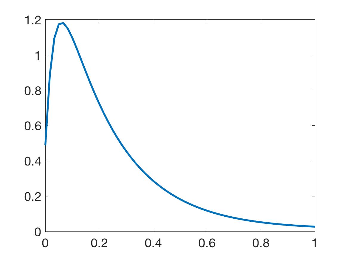 Figure 1
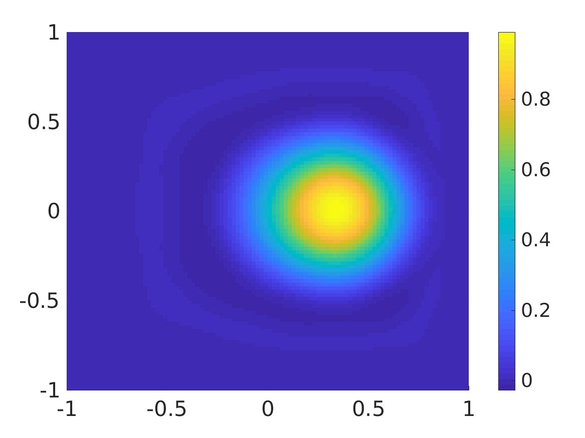 Figure 2
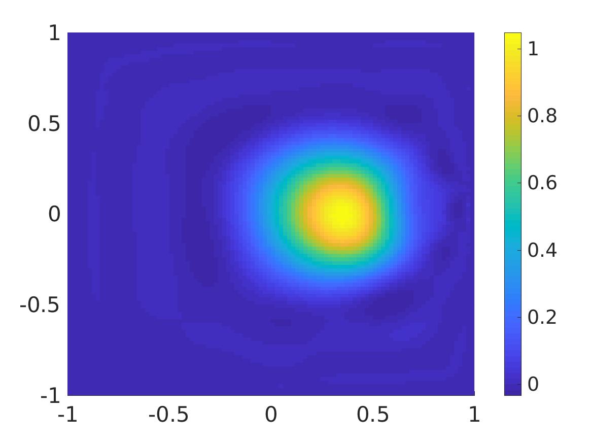 Figure 3
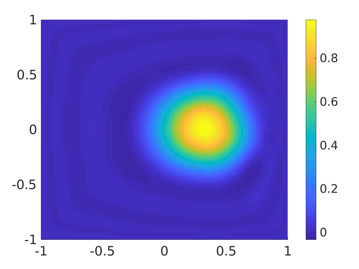 Figure 4
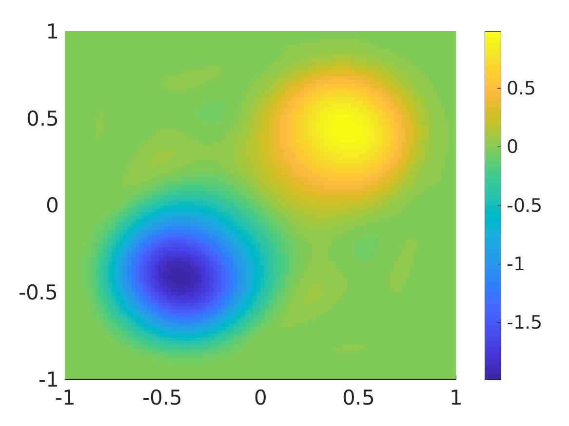 Figure 5
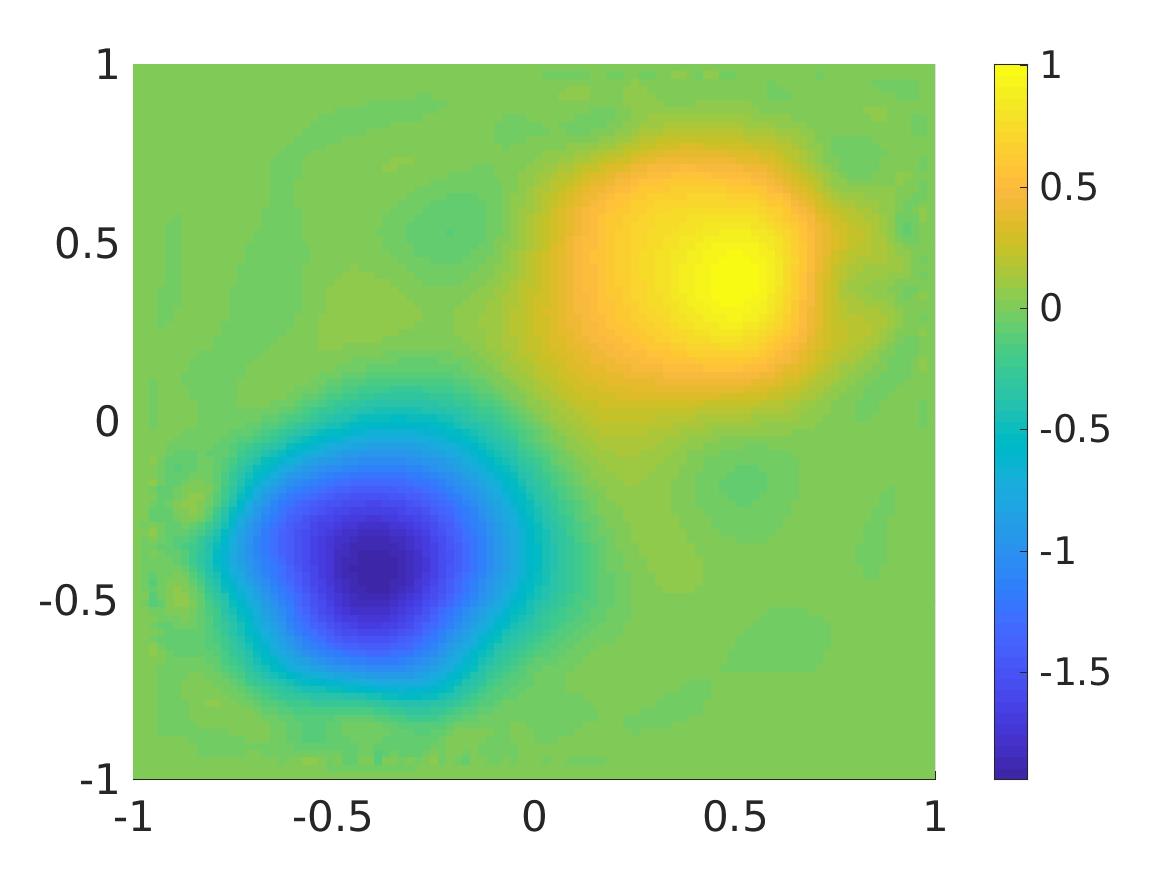 Figure 6
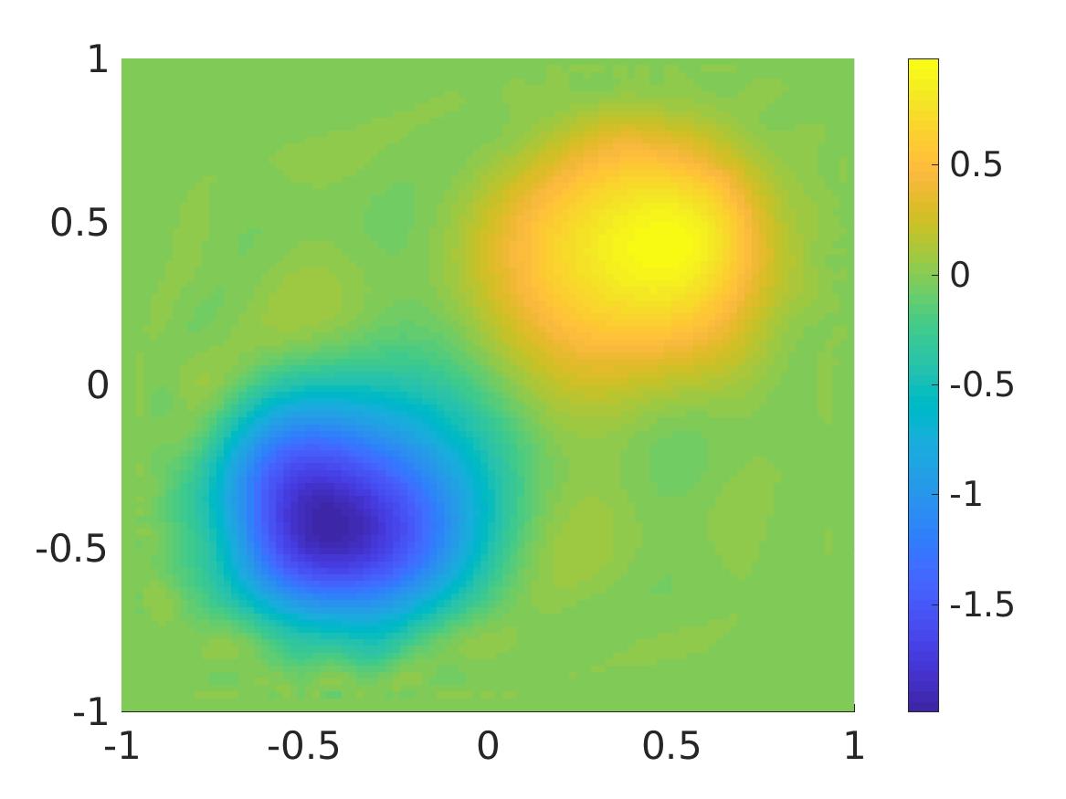 Figure 7
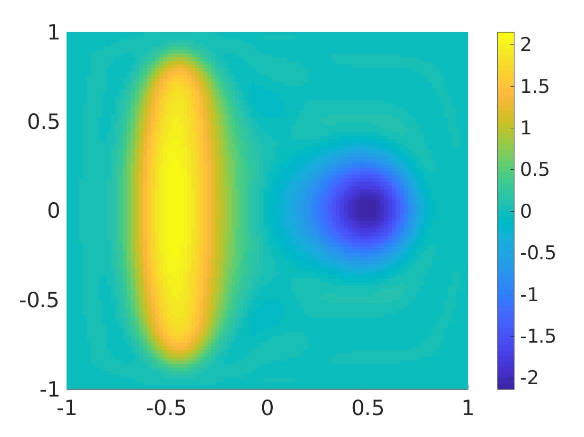 Figure 8
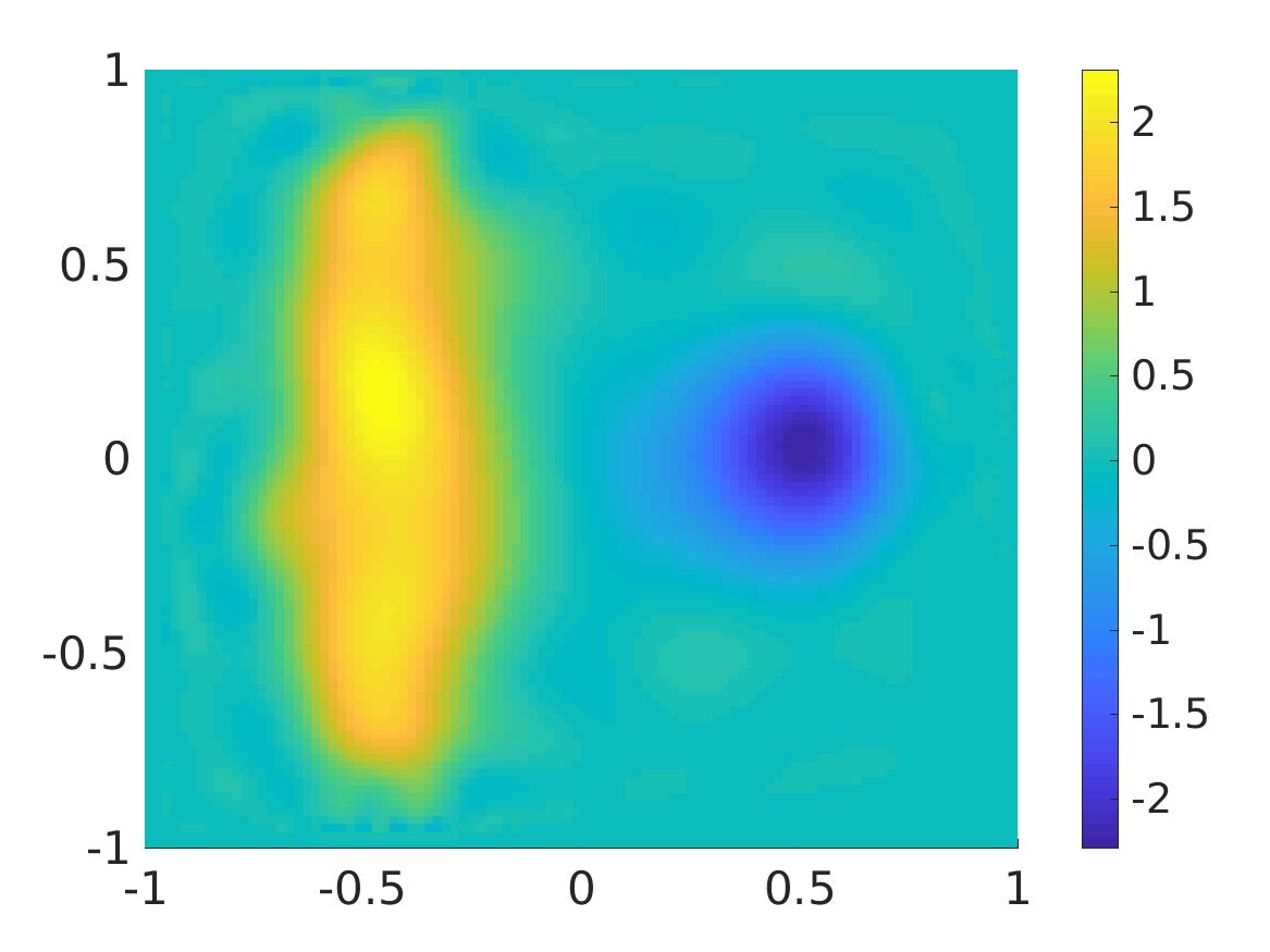 Figure 9
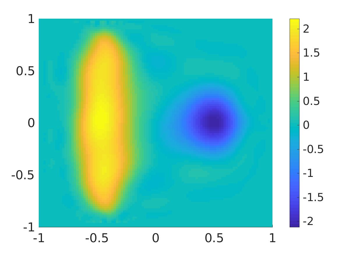 Figure 10
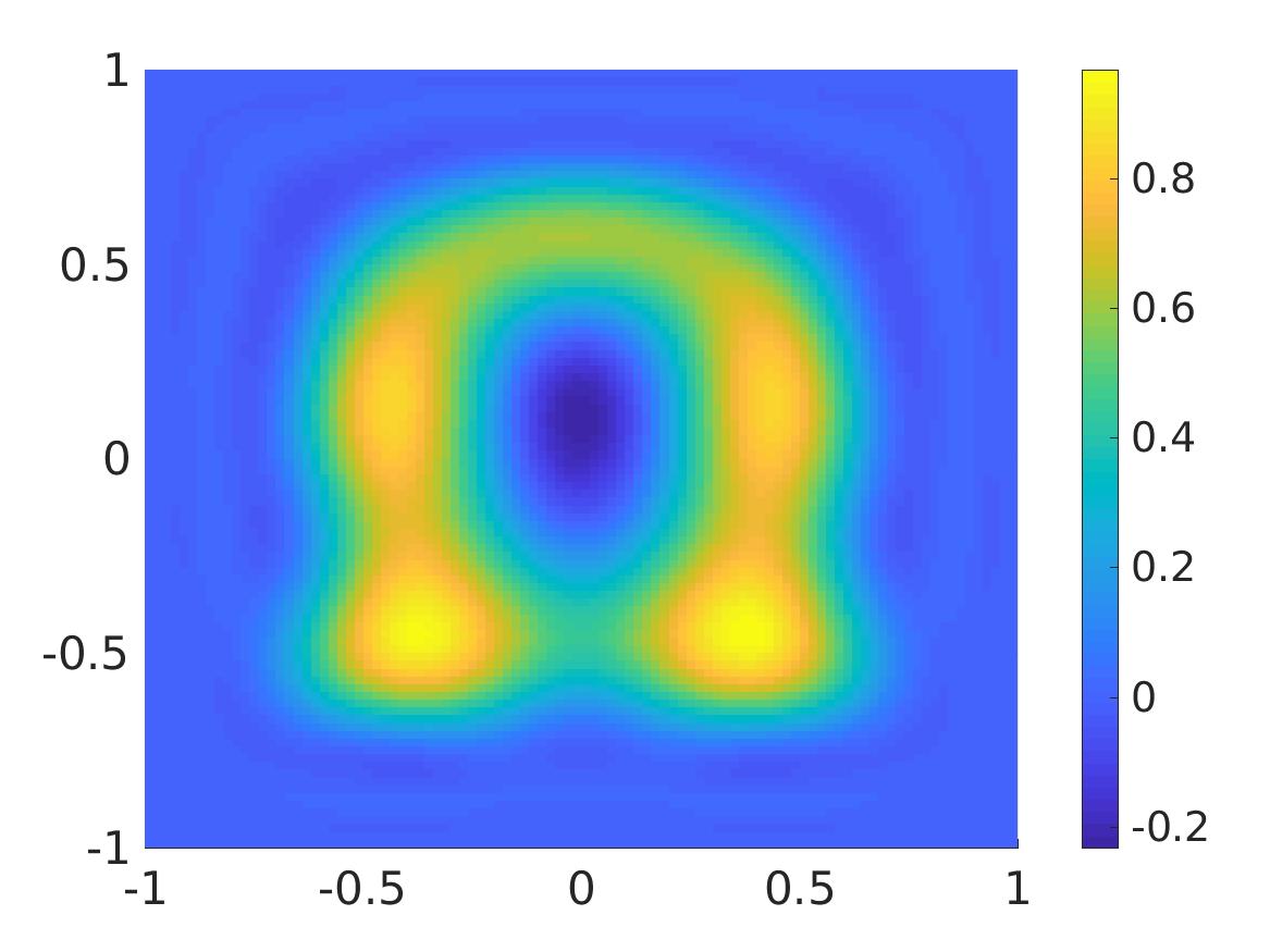 Figure 11
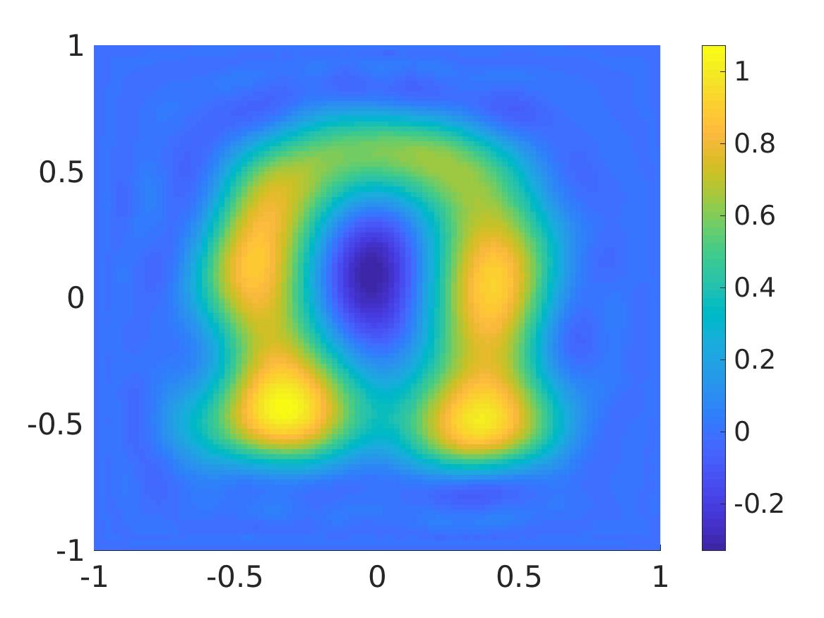 Figure 12
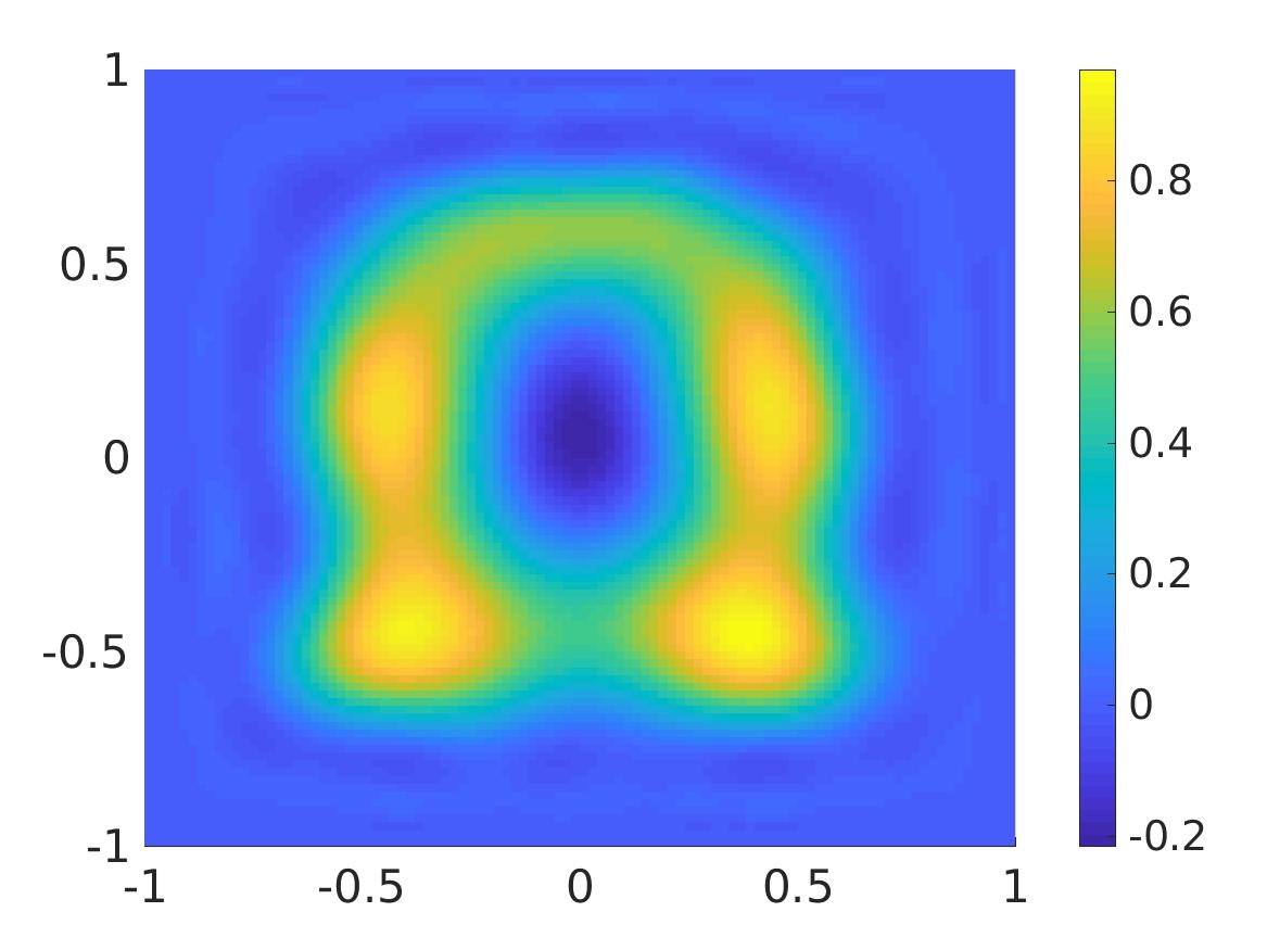 Figure 13
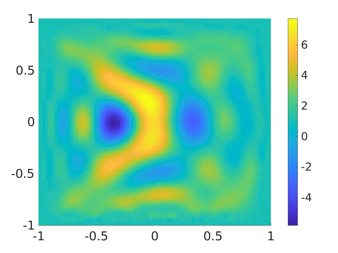 Figure 14
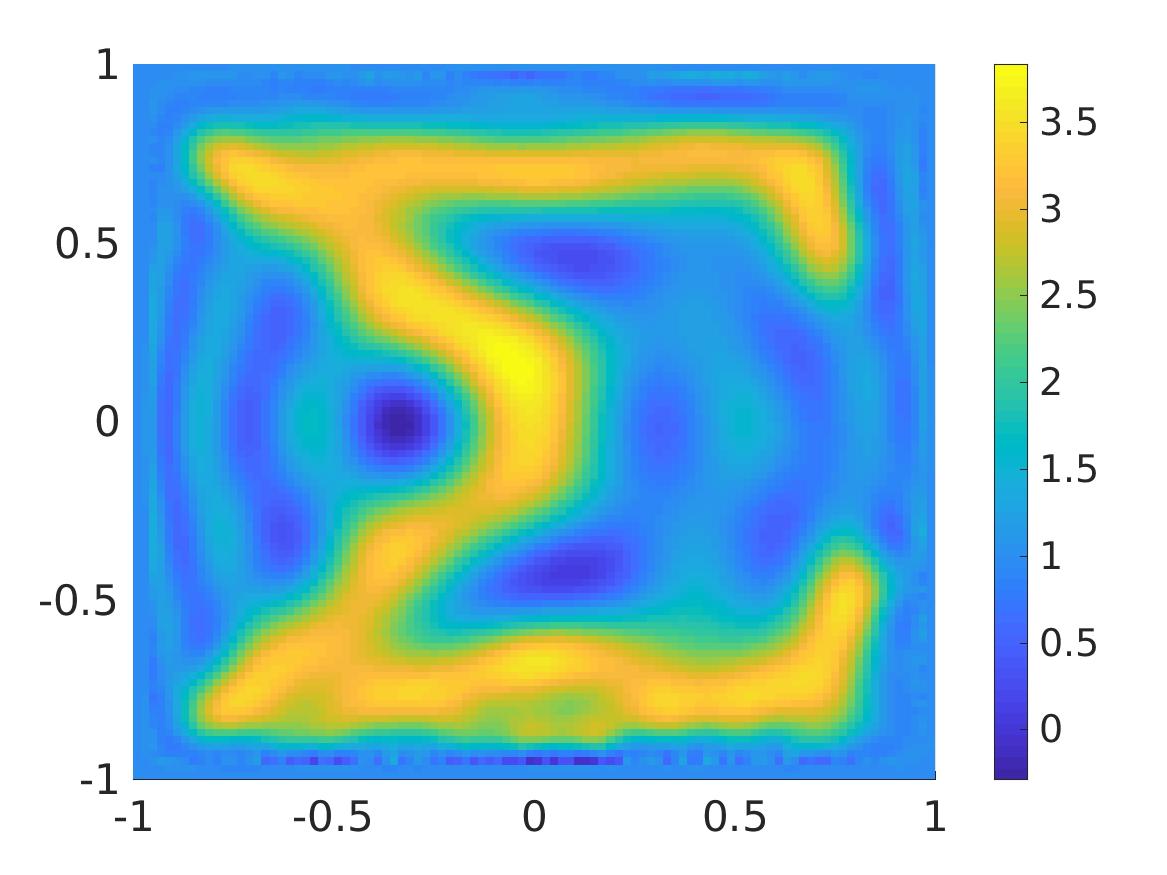 Figure 15
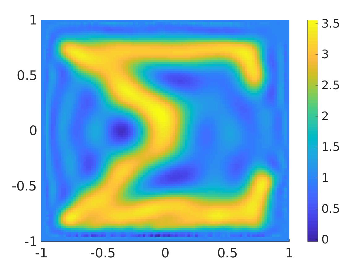 Figure 16
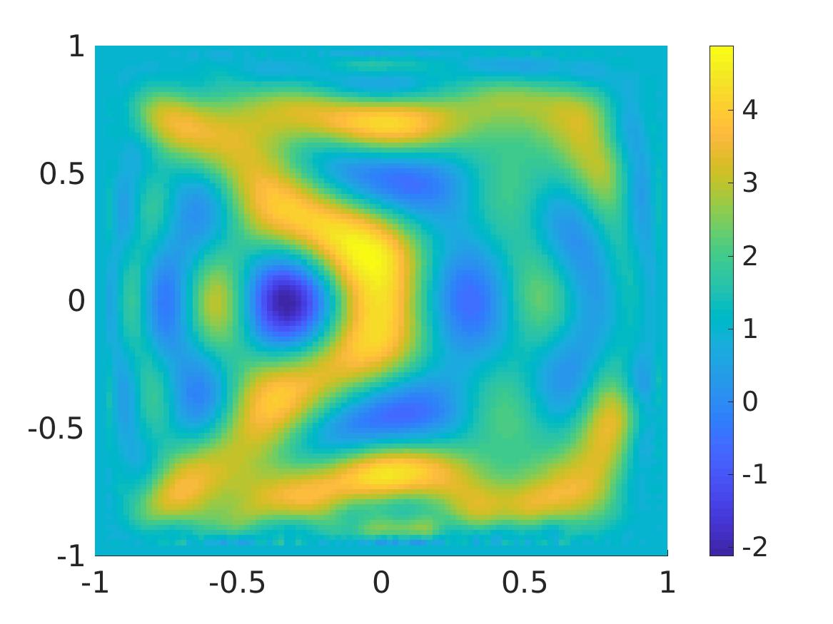 Figure 17
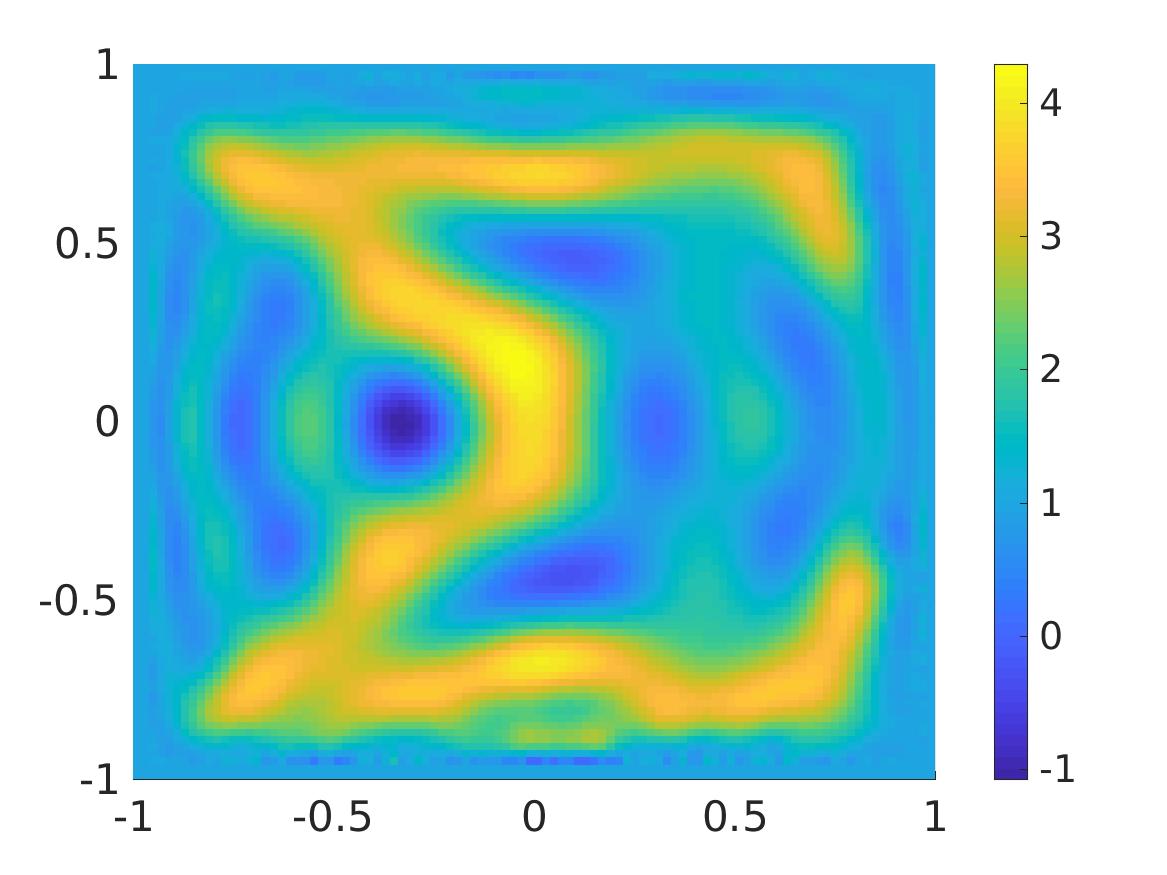 Figure 18
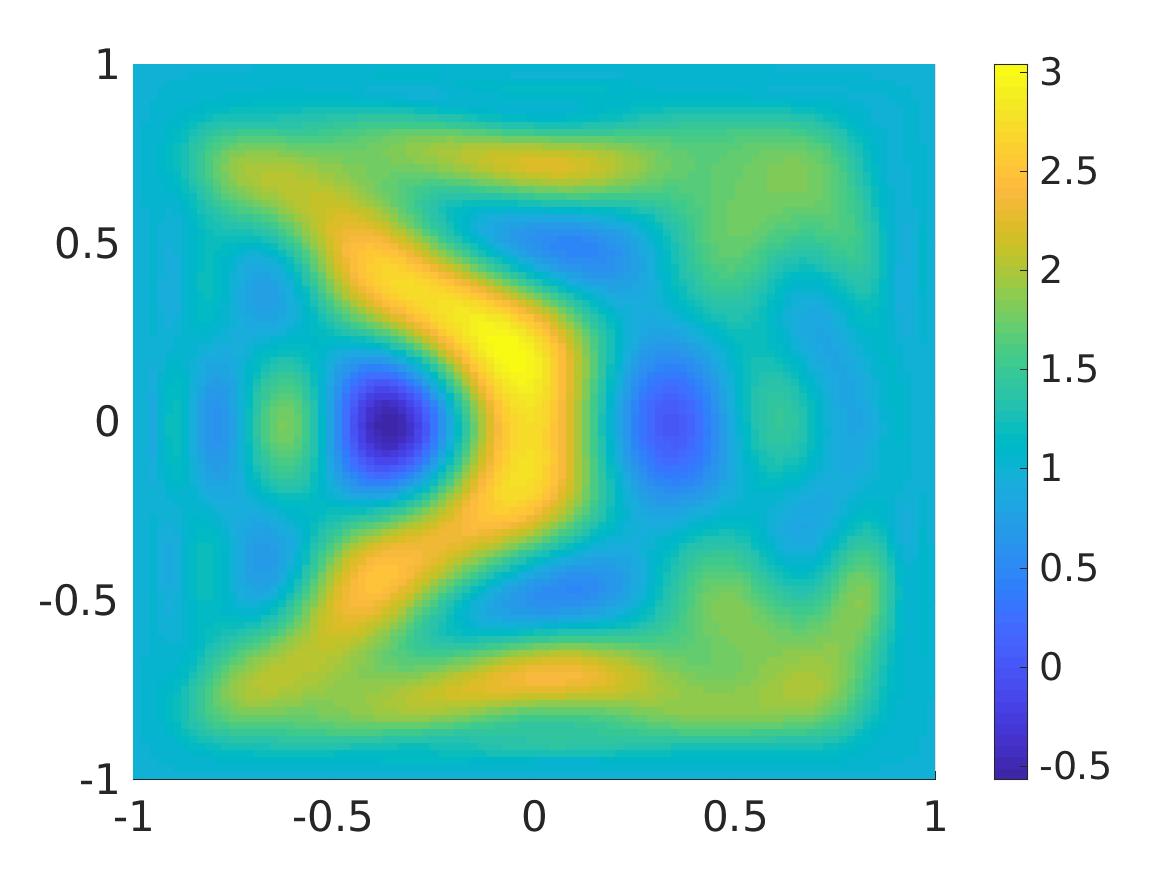 Figure 19
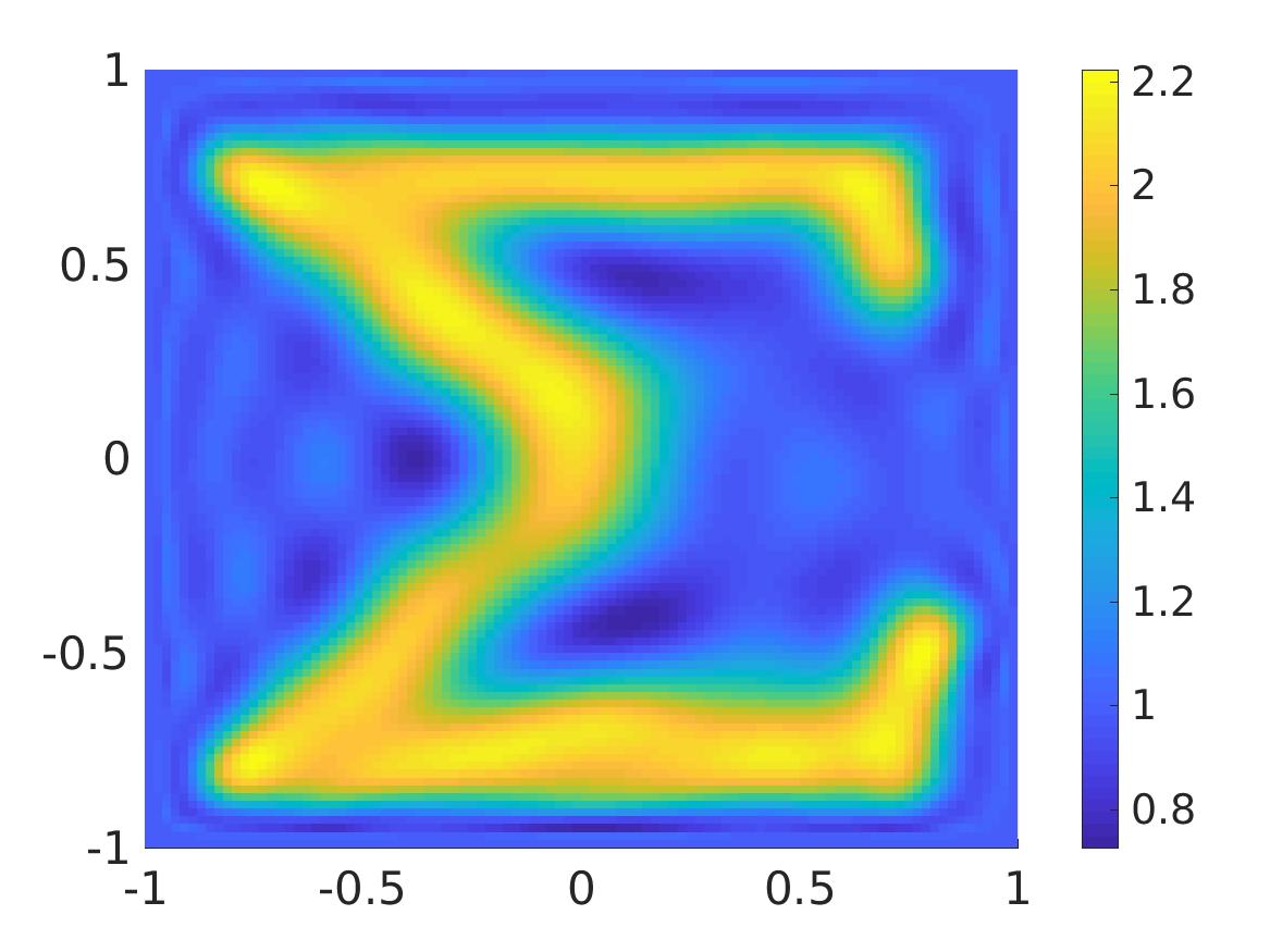 Figure 20
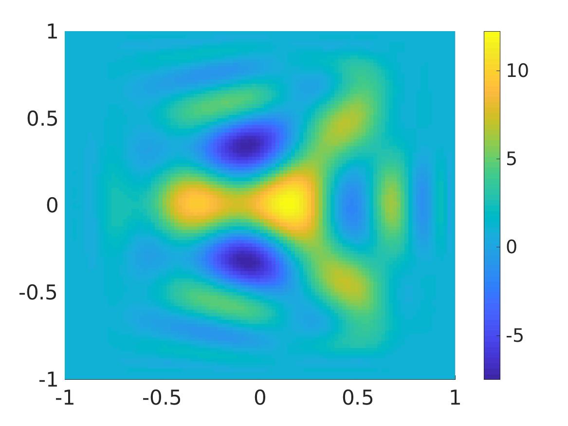 Figure 21
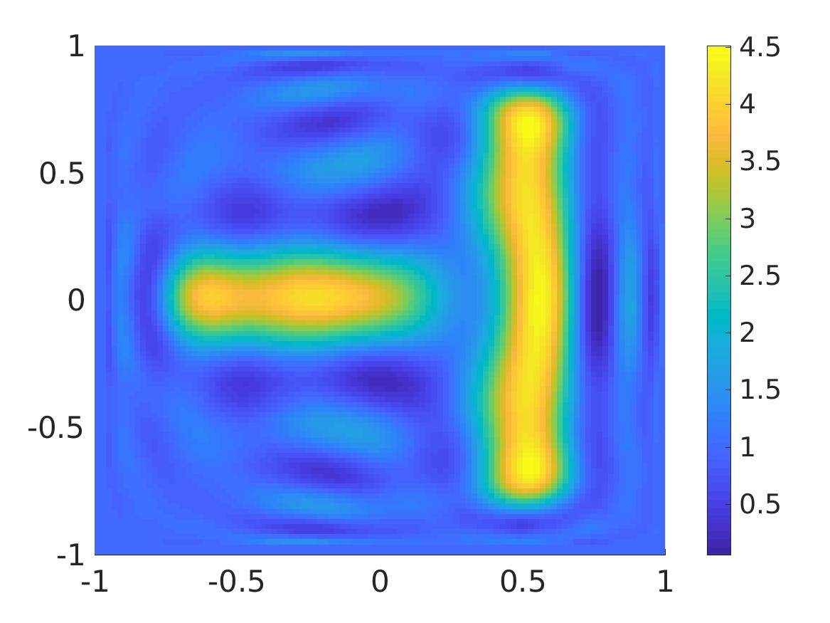 Figure 22
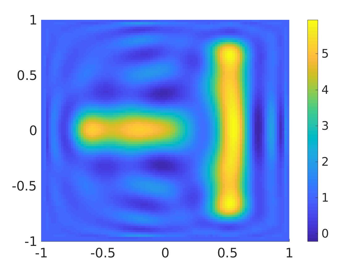 Figure 23
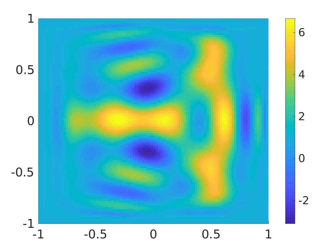 Figure 24
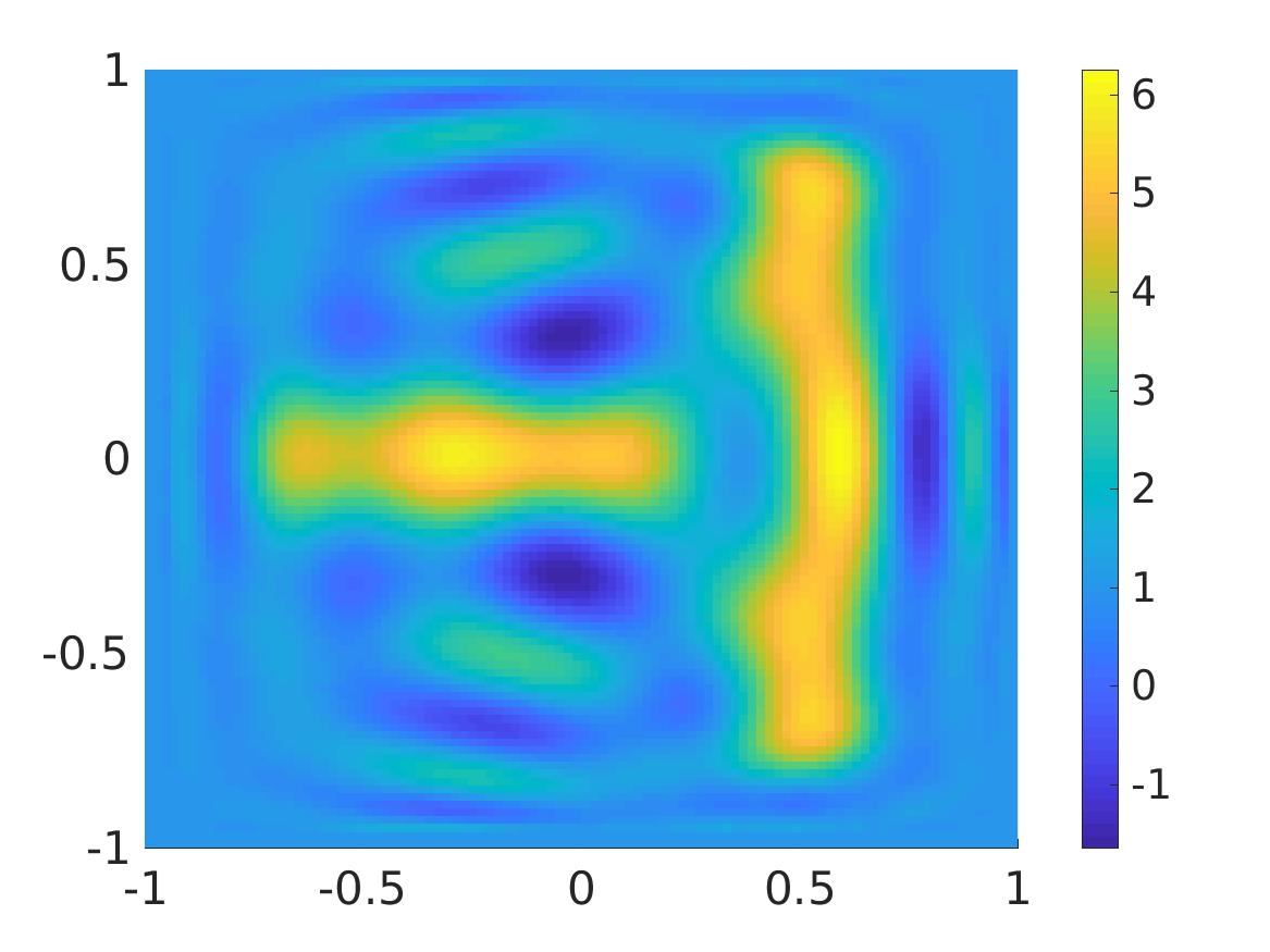 Figure 25
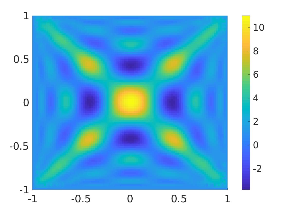 Figure 26
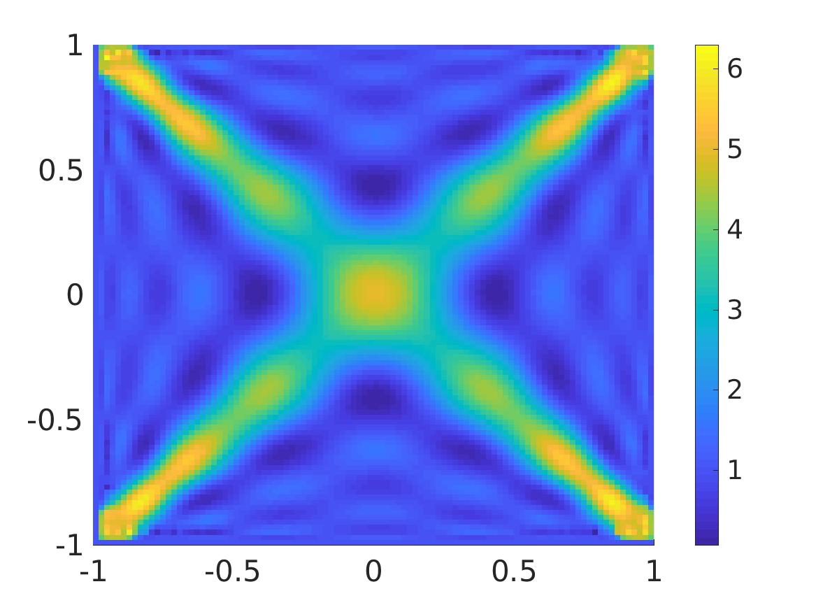 Figure 27
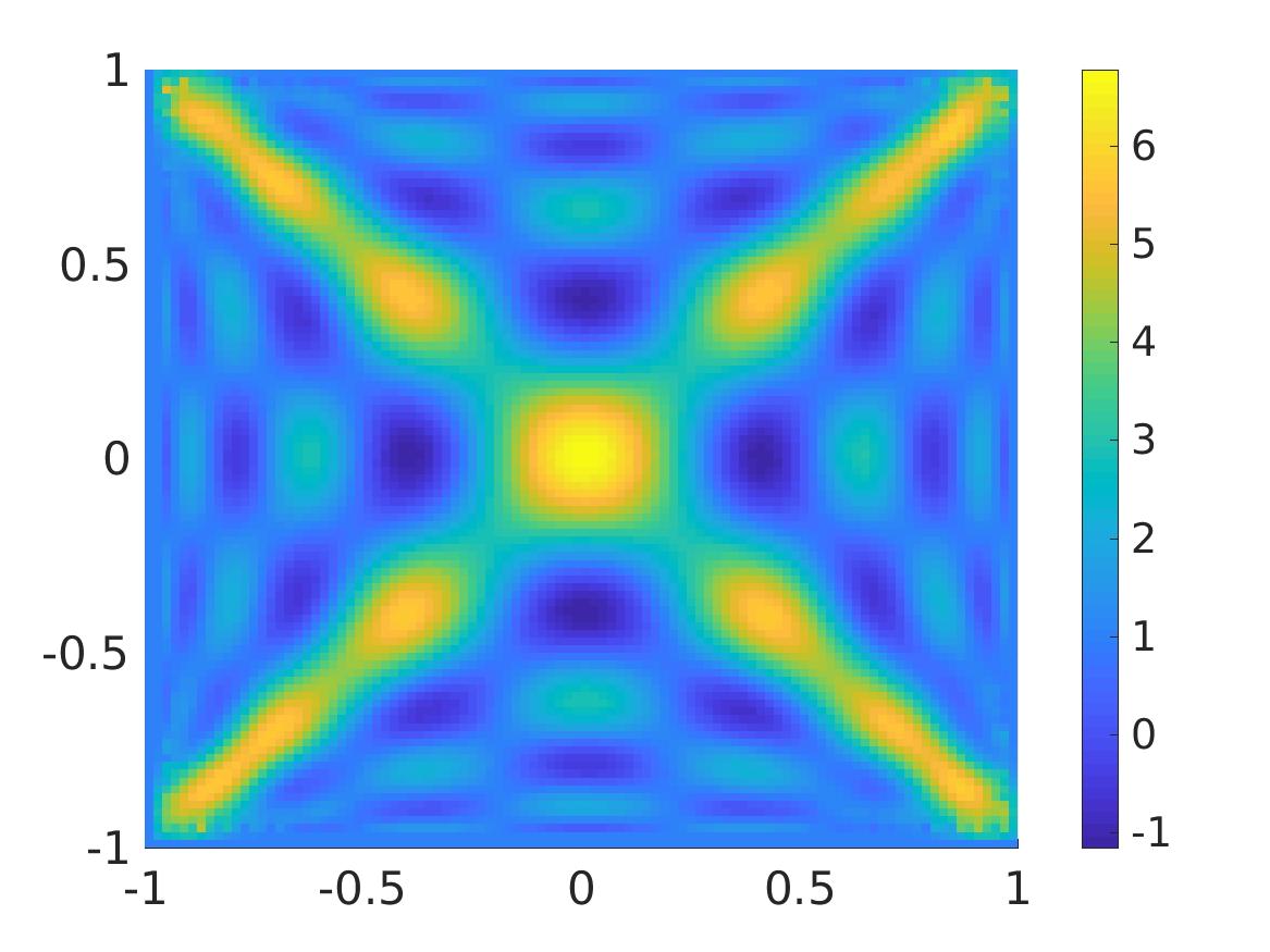 Figure 28
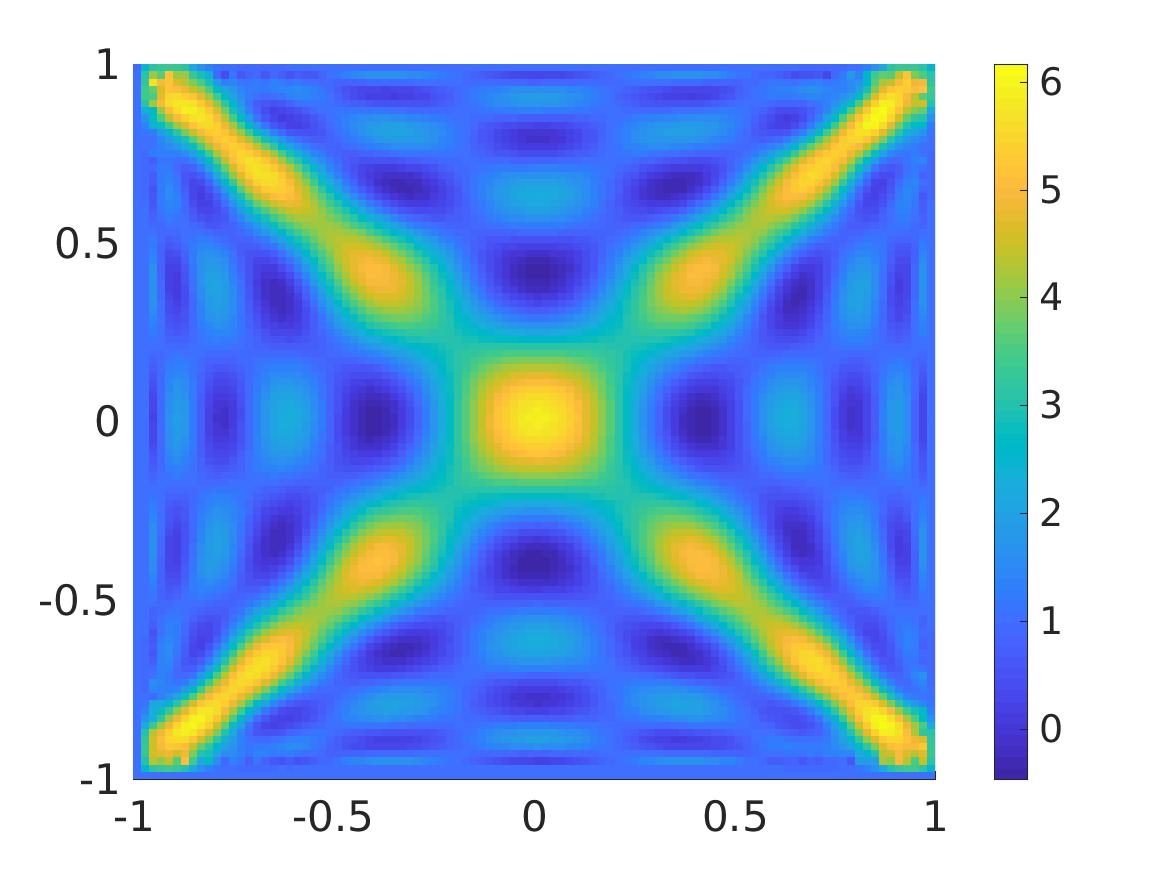 Figure 29
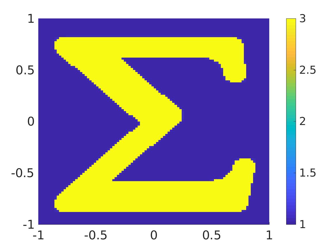 Figure 30
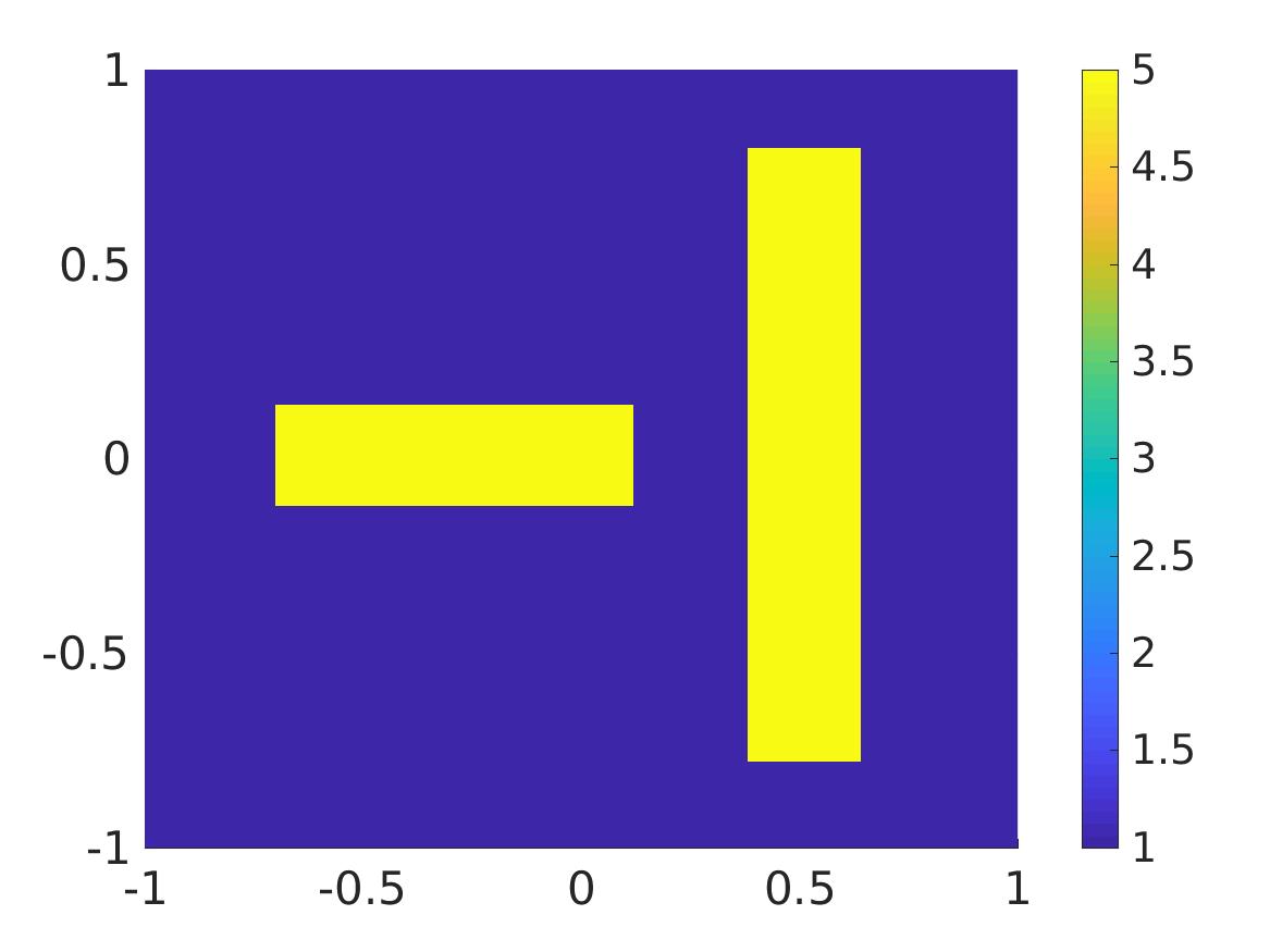 Figure 31
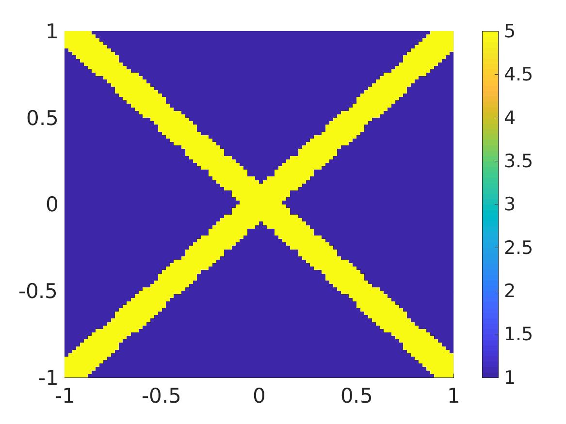 Figure 32
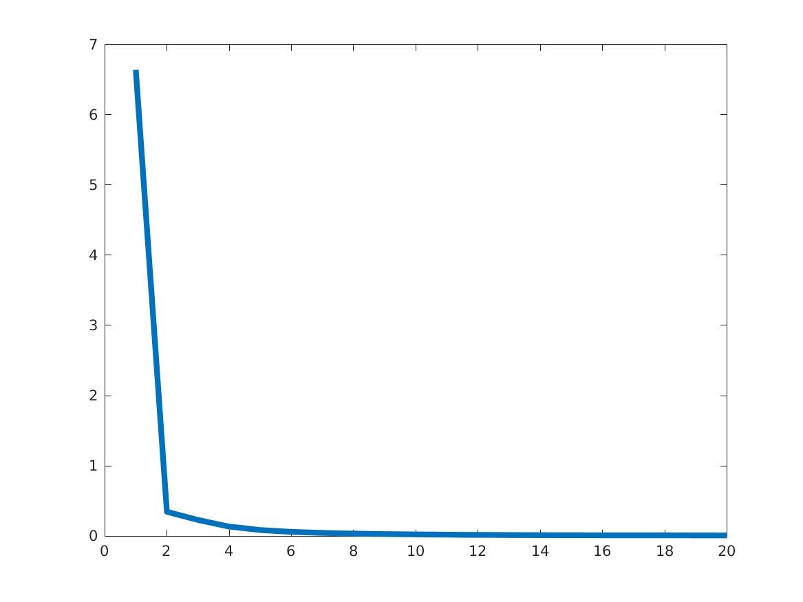 Figure 33
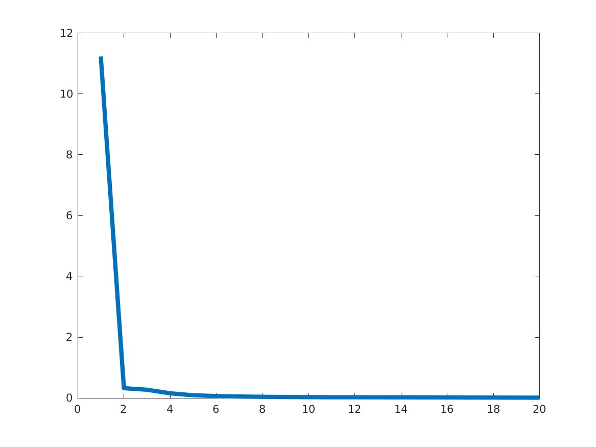 Figure 34
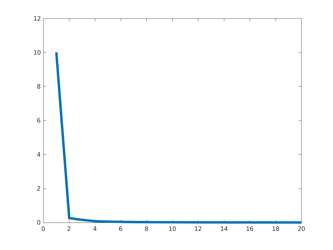 Figure 35
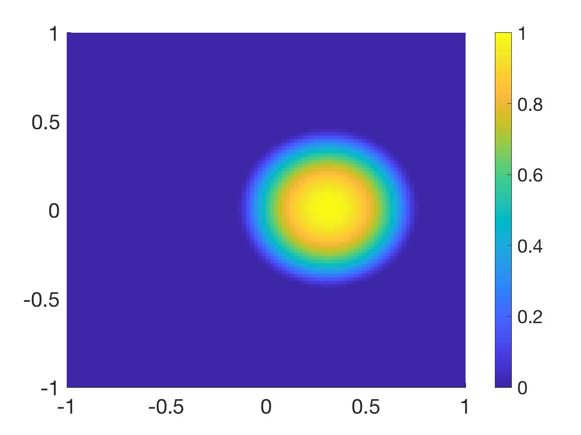 Figure 36
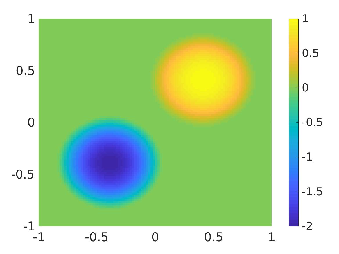 Figure 37
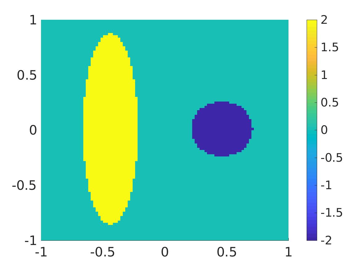 Figure 38
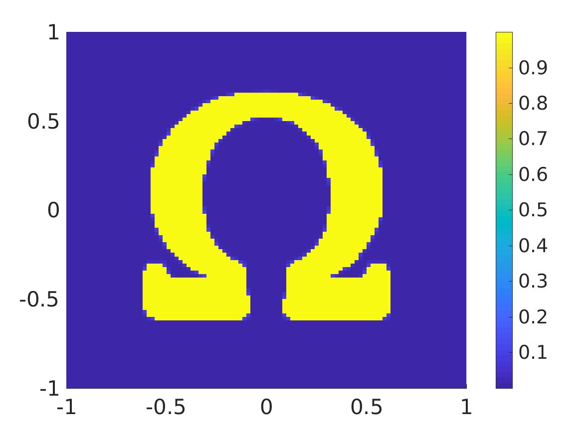 Figure 39
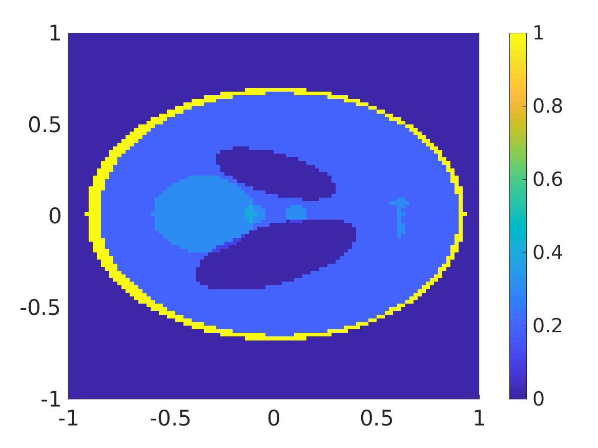 Figure 40
| Inclusion | noise level | extreme valuetrue | extreme valuecomp | |
|---|---|---|---|---|
| 1 | 0% | 1 | 0.988 | 1.2% |
| 2 | 0% | -2 | -1.99 | 0.5% |
| 1 | 5% | 1 | 0.984 | 1.6% |
| 2 | 5% | -2 | -1.987 | 0.65% |
| 1 | 10% | 1 | 1.004 | 0.4% |
| 2 | 10% | -2 | -1.938 | 3.1% |
| Inclusion | Noise level | Extreme valuetrue | Extreme valuecomp | |
|---|---|---|---|---|
| 1 | 0% | 2 | 2.151 | 7.5% |
| 2 | 0% | -2 | -2.133 | 6.7% |
| 1 | 5% | 2 | 2.211 | 10.6% |
| 2 | 5% | -2 | -2.117 | 5.9% |
| 1 | 10% | 2 | 2.312 | 15.6% |
| 2 | 10% | -2 | -2.29 | 14.5%% |
Peer Reviews
No public reviews on file for this paper yet. If you reviewed it on a platform where reviews are public (OpenReview, ICLR, NeurIPS, ICML), you can paste yours below so the community can read it here.
Videos
No videos yet. Explain this paper in a talk, walkthrough, or lecture? Add one.
A numerical method for an inverse source problem for parabolic equations and its application to a coefficient inverse problem
Phuong Mai Nguyen Department of Mathematics and Statistics, University of North Carolina Charlotte, Charlotte, NC, 28223, USA, [email protected]
Loc Hoang Nguyen Department of Mathematics and Statistics, University of North Carolina Charlotte, Charlotte, NC, 28223, USA, [email protected], corresponding author
Abstract
Two main aims of this paper are to develop a numerical method to solve an inverse source problem for parabolic equations and apply it to solve a nonlinear coefficient inverse problem. The inverse source problem in this paper is the problem to reconstruct a source term from external observations. Our method to solve this inverse source problem consists of two stages. We first establish an equation of the derivative of the solution to the parabolic equation with respect to the time variable. Then, in the second stage, we solve this equation by the quasi-reversibility method. The inverse source problem considered in this paper is the linearization of a nonlinear coefficient inverse problem. Hence, iteratively solving the inverse source problem provides the numerical solution to that coefficient inverse problem. Numerical results for the inverse source problem under consideration and the corresponding nonlinear coefficient inverse problem are presented.
Key words. parabolic equation, inverse source problem, coefficient inverse problem, numerical method, quasi-reversibility method
AMS Classification 35R30, 35K20
1 Introduction
The area of inverse source problems has many applications and it, therefore, attracts the attention of the scientific community, see e.g., [14, 13, 15, 16, 17, 29, 32, 34, 35]. The solutions of inverse source problems can be used to directly detect the source even when the source is inactive after a certain time. Here, we name some examples. In the case of the parabolic equation, the problem plays an important role in identifying the pollution sources in a river or a lake [14]. In the case of elliptic equations, the inverse source problem has applications in electroencephalography [1, 13]. In the case that the data are generated by an acoustic source, the governing equation is the hyperbolic one and the problem addresses ultrasonics imaging and photoacoustic tomography [1, 13]. In this paper, we propose a numerical method to solve an inverse source problem for parabolic equations. This problem is the linearization of a nonlinear coefficient inverse problem. Therefore, we can use it to solve a coefficient inverse problem.
Let be a bounded domain in , , with smooth boundary . Let be a function in the class . Consider the function , , that is governed by the following initial value problem
[TABLE]
where is an elliptic operator independent of the time and is the source function. The aim of this paper is to solve the following inverse source problem.
Problem 1.1** (Inverse source problem for parabolic equations).**
Let be a positive number. Assume the function , , is known and does not vanish at any point in . Determine the function , , from the measurement of the following data
[TABLE]
for all and
The uniqueness of Problem 1.1 when the source function is a combination of some Dirac functions is confirmed in [14] and a numerical method to reconstruct this source is studied in [2]. We also draw the reader to the conditional stability in [20, 30]. In the case when the governing equation is the heat equation and the source function does not depend on the second variable, a reconstruction formula is provided in [32]. Another related problem is the inverse problem of reconstructing the initial condition for parabolic equation. This problem is very important and interesting, see [31, 36, 33, 27, 38] for theoretical results and numerical methods. In the current paper, we introduce the following approach to solve Problem 1.1. We derive from a governing equation a new equation involving only one unknown. The solution to that equation will directly provide the knowledge of the desired source function. However, that equation is not a standard partial differential equation. In fact, it involves the initial condition of itself. We prove the stability of the inverse source problem based on the projection of this equation on a finite dimensional space. A theory to solve this partial differential equation is not available yet. To solve this equation, we employ the quasi-reversibility method. This method was first introduced by Lattès and Lions [28]. It is used to computed numerical solutions to ill-posed problems for partial differential equations. Due to its strength, since then, the quasi-reversibility method attracts the great attention of the scientific community see e.g., [4, 6, 7, 8, 11, 12, 18, 26, 21, 34]. We refer the reader to [22] for a survey on this method. The solutions of partial differential equations due to the quasi-reversibility method are called regularized solution in the theory of ill-posed problems [37]. The convergence of the regularized solution to the true one for three main types of partial differential equations is well-known [22]. Recently, in [34], the second author proved a Lipchitz convergence of quasi-reversibility method for the hyperbolic operator that involves Volterra integrals. The proof for a Lipchitz convergence of the quasi-reversibility method for the parabolic operator including the initial condition when this initial condition takes some particular forms will be proved in our near future publication.
An application of the inverse source problem in this paper is to solve a coefficient inverse problem for the heat equation. Given an initial guess of the coefficient, we show that our inverse source problem is a linear “perturbation” of that nonlinear coefficient inverse problem near that initial guess. Hence, by repeatedly solving our inverse source problem, we can obtain the solution to the coefficient inverse problem, see Section 6 for details. It is worth mentioning that the optimal control method to solve nonlinear coefficient inverse problem is widely used [5, 9, 10, 19, 39] which provide good numerical results with reasonable initial guesses. We also refer the reader to [3, 23] for the convexification method and numerical results in 1D.
The paper is organized as follows. We propose an algorithm to solve Problem 1.1 in Section 2. In section 3, we study the stability of Problem 1.1 in an approximation context. Next, in Section 4, we present the details about the implementation of our algorithm. In Section 5, we show some numerical solutions to the inverse source problem. In Section 6, we solve the nonlinear coefficient inverse problem from which the inverse source problem above arises. Section 7 is for concluding remarks.
2 The inversion method
Define the function
[TABLE]
Since does not depend on , it follows from the partial differential equation in (1.1) that
[TABLE]
for all The initial condition for the function can be computed as
[TABLE]
which implies
[TABLE]
Substituting this into (2.2), we obtain
[TABLE]
for all , Note that equation (2.4) does not depend on the function .
Problem 1.1 becomes the problem of computing the function that satisfies (2.4) and the lateral Cauchy conditions
[TABLE]
for all
Remark 2.1**.**
We consider the function as our “indirect” data. In this paper, we test our method with noisy data where is the noise level and is the uniformly distributed random number taking values in In this paper, and
Remark 2.2**.**
Our main idea when deriving (2.4) is that we want to eliminate one unknown so that we can arrive at the situation of one unknown and one equation. This strategy was applied in our research group in many publications; see e.g., [25, 35, 34]. Among them, the most similar idea to derive (2.4) is in [34] when the source term of a hyperbolic equation is eliminated. The main difference from (2.4) is that the corresponding equation in [34] is an integro-differential equation, which is not applicable in the current paper.
Assume that is known. Then, the desired function is computed via (2.3). However, due to the presence of the term , equation (2.4), together with the lateral data in (2.5), is not a standard partial differential equation. A theortical method to solve it is not yet available. We solve (2.4) and (2.5) by the quasi-reversibility method. Define the operator
[TABLE]
for all function . Given we minimize the functional
[TABLE]
subject to the constraints in (2.5).
The following proposition guarantees that has a unique minimizer in .
Proposition 2.1**.**
Assume that the set
[TABLE]
is nonempty. Then, for each the function has a unique minimizer in .
The proof of this proposition follows the proof of Proposition 3.1 in [35] for the time independent case. We present the proof for the time dependent case here for the connivence of the reader.
Proof of Proposition 2.1.
Let be a function in . Denote by the space Introduce . Then, minimizing for in is equivalent to minimizing for in If is a minimizer of in , then, by the variational principle,
[TABLE]
which is equivalent to
[TABLE]
The left hand side of (2.8) defines a new inner product in . We have and for some constant due to the trace theory and the assumption that is a second order elliptic operator. Hence, is equivalent to the standard inner product of . On the other hand, the right hand side of (2.8) is a bounded linear operator defined on . The existence and the uniqueness of a function satisfying (2.8) follows from the Riesz representation theorem. ∎
Remark 2.3**.**
*The unique minimizer of is call the regularized solution to (2.4) and (2.5). *
Our method to solve Problem 1.1 is summarized in Algorithm 1. In practice, we implement Algorithm 1 in the finite difference scheme. We present the implementation of Algorithm 1 with the finite difference method in the Section 4.
3 A Lipschitz estimate based on a truncation of the Fourier series
Let be an orthonormal basis of For each , we can write
[TABLE]
where is the function defined in (2.1). Here,
[TABLE]
Approximate the series in (3.1) by
[TABLE]
for for some number . We also write
[TABLE]
Plugging (3.3) and (3.4) into (2.4), we have
[TABLE]
Multiply both side of the equation above by for each and then integrate the resulting equation on . We obtain
[TABLE]
for all Define . It follows by (3.5) and the fact that that the vector valued function satisfies the system
[TABLE]
where is a matrix valued function given by
[TABLE]
Since is a smooth function, so is . By a standard compact argument for elliptic equation, we can find a constant depending only on , and such that
[TABLE]
It follows from (1.1), (1.2), (2.1) and (3.2) that
[TABLE]
on . Hence, by (3.7),
[TABLE]
Using (3.3), we have
[TABLE]
As a result, using (2.3) and the trace theory, we get
[TABLE]
In summary, we have proved the following theorem.
Theorem 3.1**.**
Assume that the function is well-approximated by the Fourier sum as in (3.3) for some integer where is the solution to (1.1). Then, there exists a constant depending only on , and such that
[TABLE]
Theorem 3.1 implies the Lipschitz stability for Problem 1.1 in the finite dimensional space spanned by . Studying the stability when tends to is extremely challenging and is out of the scope of this paper.
Remark 3.1**.**
The assumption about the well-approximation in Theorem 3.1 is verified numerically in some recent works of our research group. This verification for elliptic equation can be found in [35] and the one for parabolic equation is in [31]. In those papers, the basis is taken from [24].
4 The finite difference method to find the regularized solution
In this section, the domain is set to be a square in ; i.e,
[TABLE]
where is a positive number. Let and be positive integers. Set and We define a set of grid points on
[TABLE]
and define a uniform partition on the time domain as
[TABLE]
For the simplicity in implementation, in this section, we modify the norm in the regularization term in (2.7) to the norm. In other words,
[TABLE]
for all
Remark 4.1**.**
We replace the norm in regularization term by the –norm because the –norm is easier to implement. On the other hand, we have not observed any instabilities probably because the number of grid points we use is not too large and all norms in finite dimensional spaces are equivalent.
Remark 4.2** (The choice of ).**
We observe numerically that if is larger than , the reconstructed images of the source function are good but the reconstructed values are low and if , our method breaks down. We choose in all our numerical tests. Note that this choice of is independent of the noise level, which is, in practice, supposed to be unknown.
The finite difference version of still named as , reads
[TABLE]
Here, is the approximation of in the finite difference scheme and is the finite difference gradient. From now on, for the simplicity and to minimize the effort of writing computational code, we consider the case
[TABLE]
for some function in In this case,
[TABLE]
and
[TABLE]
for all and Introduce the dimensional vector , , whose entry is given by
[TABLE]
where
[TABLE]
Then, we can rewrite (4.2) as
[TABLE]
where the matrix is described as follows. For each with and ,
the entry is given by ; 2. 2.
the entry is given by where for ; 3. 3.
the entry is given by where for ; 4. 4.
the entry is given by where for ; 5. 5.
the other entries are [math].
We next define the matrices and such that . For each with and ,
the entry of and is given by ; 2. 2.
the entry of is given by for ; 3. 3.
the entry of is given by for ; 4. 4.
other entries are
The finite difference version of , defined in (4.1), becomes
[TABLE]
Hence, due to (4.3), since is a minimizer of , satisfies the equation
[TABLE]
We next consider the boundary conditions for in (2.5). In the finite difference scheme, the first condition in (2.5) reads for
[TABLE]
for all and or and . Therefore, due to (4.3), we can write this condition as
[TABLE]
where is defined as follows. For
the entry of is set to be if for some , or , ; 2. 2.
the other entries of are [math].
The second condition in (2.5) is rewritten as
[TABLE]
where the vector is the lineup version of the data
[TABLE]
for all and or and and the matrix is defined as follows. For all ,
the entry of is if for , or , ; 2. 2.
the entry of is if for , and ; 3. 3.
the entry of is if for , and ; 4. 4.
the entry of is if for , and ; 5. 5.
the entry of is if for , and ; 6. 6.
the other entries of are 0.
Combining (4.5), (4.6) and (4.7), we obtain
[TABLE]
Since is a small number, it is acceptable that we modify the equation above by a more “stable” one
[TABLE]
The analysis in this section is summarized in the following proposition.
Proposition 4.1**.**
The source function can be computed by
solve (4.8) for , the “line up” version of ; 2. 2.
compute the function using (4.3); 3. 3.
calculate .
5 Numerical results
We test our numerical method when and therefore, is Also, we choose , see the Remark 1 for this choice of .
Remark 5.1** (Choose ).**
We numerically choose by examining the norm of the data on as a function in . Define
[TABLE]
The graph of the function is displayed in Figure 1, showing that the data is largest on . This means the data contains most important information about the source in this interval. We therefore choose for all of our numerical tests.
We chose and in this section. In all tests, the known function is chosen as
[TABLE]
and the known function is set to be
[TABLE]
In this section, we show the following numerical results.
Test 1. In this test, the true source function is smooth and given by
[TABLE]
The numerical result for this test is displayed in Figure 2.
It is evident that our method well reconstructs the source function . The location and shape of the circular “inclusion” can be identified. The true maximum value of the inclusion is . The reconstructed maximum value of the inclusion is computed with small errors. In fact,
when and the coresponding relative error is ; 2. 2.
when and the coresponding relative error is ; 3. 3.
when and the coresponding relative error is .
Test 2. We test our method for the case when is given by the smooth function
[TABLE]
In this test, the true source function has a negative “inclusion” and a positive one. The numerical results for this test are displayed in Figure 3.
The true and computed local extreme values of the source function at two inclusions are displayed in Table 1. This table show that our method is stable with respect to noise.
Test 3. We next check the case when the source function is not smooth. In this case, we consider the piecewise constant function
[TABLE]
The graph of the function has two “inclusions” with different shapes, a disk and an ellipse. The graphs of the true and computed source function are displayed in Figure 4.
The reconstruction of the image of the source function in this test is acceptable. Table 2 shows the strength of our method in the sense that we can reconstruct the values of those two inclusions with acceptable error.
Test 4. We test the nonsmooth true source function again with a complicated support. The true function is the characteristic function of the letter The numerical results for this test are shown in Figure 5.
Note that the maximal value of the reconstructed functions are acceptable. When (relative error 3%). When (relative error 3%). When (relative error 7.3%).
Remark 5.2**.**
Despite of the presence of the initial condition in equation (2.4), it is evident that the quasi-reversibility method provides good numerical results with small relative errors.
6 Application to a coefficient inverse problem
In this section, we propose a numerical method to solve a severely ill-posed nonlinear coefficient inverse problem.
6.1 The problem statement
Problem 1.1 arises from a coefficient inverse problem for parabolic equations. For the simplicity, consider the problem of determining the coefficient from the measurements of on where, is the solution of the following problem
[TABLE]
Assume that the initial condition for all and the boundary condition satisfying for all in Consider the following nonlinear inverse problem.
Problem 6.1**.**
Let Determine the coefficient , from the measurement of
[TABLE]
for all
Problem 6.1 and its related versions are studied intensively. Up to the knowledge of the author, the widely used method to solve this problem is the optimal control approach, see e.g., [5, 9, 10, 19, 39] and references therein. The main drawback of this method is that the initial guess for the true solution is important to obtain numerical results. Un like this, we assume that we do not have any advanced knowledge of the true solution to Problem 6.1 and take the initial guess as a constant function.
Consider the circumstance that an initial guess for the function , named as , is known. Then, we write
[TABLE]
Denote by the function the solution of (6.1) with replacing and let . It is not hard to see that
[TABLE]
Since is an initial guess of , we can replace the function in the differential equation in (6.3) above by to obtain
[TABLE]
which leads to a particular case of Problem 1.1 with . We can compute and therefore via solving Problem 1.1 for the heat equation (6.4). Denoting the computed by and let be the solution to (6.1) with . We then find by solving Problem 1.1 for the heat equation (6.4) with replacing . The process is repeated to compute and we choose when is a fixed positive integer. We summarize this numerical method to compute in Algorithm 2.
Remark 6.1**.**
Imposing assumption (6.2), where the function is known and the unknown function is small, only plays the role of the suggestion for the “linearization” analysis. However, in the reverse direction, the numerical results show that Algorithm 2 can be applied and provide good numerical results even in the case when is far away from the function . Here, we understand by “ is far away from the function ” in two senses: (1) the complicated geometry of the true function and (2) the high contrasts.
Remark 6.2**.**
The difficulty about the presence of an initial guess can be overcome using the quasi-reversibility method. The authors of [3, 23] introduce a convex functional, which minimizer yields the solution of the problem under consideration, by combining the quasi-reversibility method and the Carleman weight functions. Numerical results in 1D are presented in [3]. It is important and interested to numerically test their method in higher dimensions.
In the next subsection, we will show some numerical results. We also display the graph of the relative difference
[TABLE]
to show the convergence of Algorithm 2.
6.2 Numerical results
We perform two numerical results due to Algorithm 2 below. In these tests, the noise level is . The background function for all
Test 5. The function is the step function taking value 3 inside a letter and otherwise. We display the obtained numerical results in Figure 6.
The reconstructed image “” meets the expectation although the initial guess is far away from the true function . The true maximal value of the function is 3 and the reconstructed one is 3.56. The relative error is
Test 6. In test 6, the function is given by
[TABLE]
The image of the function has a horizontal rectangle and a vertical rectangle. Due to the geometry and the high value, is far away from the background . We display the obtained numerical results in Figure 7. Despite of the “bad” initial guess , the rectangles can be seen after a few iterations. We note that the reconstructed images and value are improved with more iterations. The true maximum value of is 5 and the reconstructed one is 5.94. The relative error is 18.8%.
Remark 6.3**.**
We observe that with the choice of as the background constant, the first reconstructed function is poor. Then, in the next two iterations, the quality of the reconstructed function improves significantly. Figures 6f and 7f show that the sequence converges at the very fast rate.
7 Concluding remarks
In this paper, we have proposed a method to solve an inverse source problem for parabolic equations. The stability of this problem is proved in an approximation context. To compute the numerical solutions to this inverse source problem, we derived an equation whose solution directly provides the desired solution of our inverse source problem. However, this equation is not a standard parabolic equation. A theory to solve it is not yet available. We therefore employ the quasi-reversibility method to find its solution. Since the inverse source problem in this paper is a linearization of a nonlinear coefficient inverse problem, we use the proposed method to establish an iterative method to solve that nonlinear coefficient inverse problem. Numerical results were presented.
Acknowledgments
The authors sincerely appreciate Michael V. Klibanov for many fruitful discussions. The work of the second author was supported by US Army Research Laboratory and US Army Research Office grant W911NF-19-1-0044.
The reference list from the paper itself. Each links out to its DOI / PubMed record.
- 1[1] M. A. Anastasio, J. Zhang, D. Modgil and P. J. La Rivière, Application of inverse source concepts to photoacoustic tomography, Inverse Problems 23 (2007), S 21–S 35.
- 2[2] M. Andrle and A. El Badia, On an inverse source problem for the heat equation. Application to a pollution detection problem, II, Inverse Problems in Science and Engineering 23 (2015), 389–412.
- 3[3] A. B. Bakushinskii, M. V. Klibanov and N. A. Koshev, Carleman weight functions for a globally convergent numerical method for ill-posed Cauchy problems for some quasilinear PD Es, Nonlinear Anal. Real World Appl. 34 (2017), 201–224.
- 4[4] E. Bécache, L. Bourgeois, L. Franceschini and J. Dardé, Application of mixed formulations of quasi-reversibility to solve ill-posed problems for heat and wave equations: The 1D case, Inverse Problems & Imaging 9 (2015), 971–1002.
- 5[5] L. Borcea, V. Druskin, A. V. Mamonov and M. Zaslavsky, A model reduction approach to numerical inversion for a parabolic partial differential equation, Inverse Problems 30 (2014), 125011.
- 6[6] L. Bourgeois, Convergence rates for the quasi-reversibility method to solve the Cauchy problem for Laplace’s equation, Inverse Problems 22 (2006), 413–430.
- 7[7] L. Bourgeois and J. Dardé, A duality-based method of quasi-reversibility to solve the Cauchy problem in the presence of noisy data, Inverse Problems 26 (2010), 095016.
- 8[8] L. Bourgeois, D. Ponomarev and J. Dardé, An inverse obstacle problem for the wave equation in a finite time domain, Inverse Probl. Imaging 13 (2019), 377–400.