Strong Convergence of Multivariate Maxima
Michael Falk, Simone A. Padoan, Stefano Rizzelli

TL;DR
This paper extends the convergence of maxima of uniform variables to higher dimensions using copulas, showing strong convergence results that support consistent estimation in max-stable models.
Contribution
It generalizes the convergence in total variation to multivariate cases via copulas near generalized Pareto copulas, enabling robust statistical inference.
Findings
Convergence in variational distance for maxima of i.i.d. vectors.
Strong convergence results for copulas near generalized Pareto copulas.
Application to almost-sure consistency of max-stable model estimators.
Abstract
It is well known and readily seen that the maximum of independent and uniformly on distributed random variables, suitably standardised, converges in total variation distance, as increases, to the standard negative exponential distribution. We extend this result to higher dimensions by considering copulas. We show that the strong convergence result holds for copulas that are in a differential neighbourhood of a multivariate generalized Pareto copula. Sklar's theorem then implies convergence in variational distance of the maximum of independent and identically distributed random vectors with arbitrary common distribution function and (under conditions on the marginals) of its appropriately normalised version. We illustrate how these convergence results can be exploited to establish the almost-sure consistency of some estimation procedures for max-stable models, using…
Click any figure to enlarge with its caption.
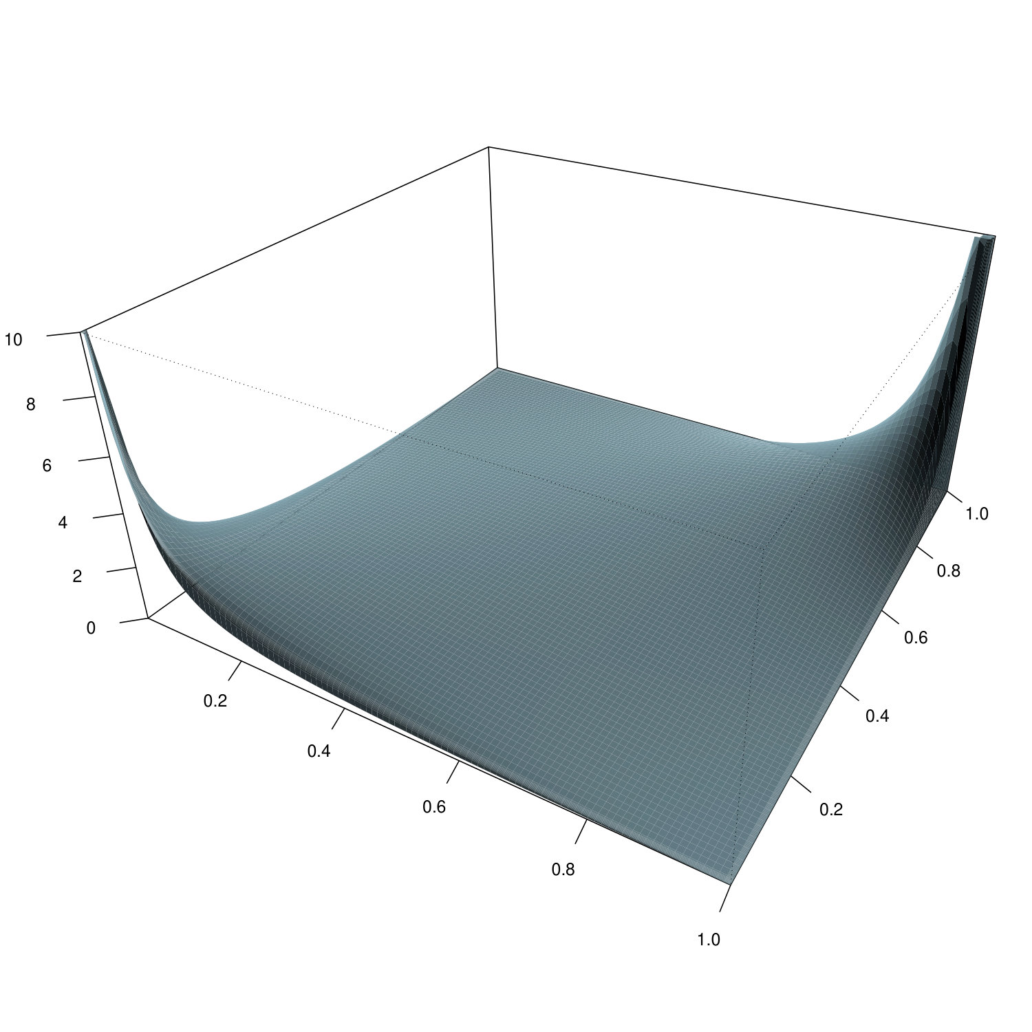 Figure 1
Peer Reviews
No public reviews on file for this paper yet. If you reviewed it on a platform where reviews are public (OpenReview, ICLR, NeurIPS, ICML), you can paste yours below so the community can read it here.
Videos
No videos yet. Explain this paper in a talk, walkthrough, or lecture? Add one.
Strong Convergence of Multivariate Maxima
Michael Falk*(1)*
Institute of Mathematics, University of Würzburg, Würzburg, Germany
,
Simone A. Padoan*(2)*
Department of Decision Sciences, Bocconi University of Milan, Milano, Italy
and
Stefano Rizzelli*(3)*
Institute of Mathematics, École Polytechnique Fédérale de Lausanne, Lausanne, Switzerland
Abstract.
It is well known and readily seen that the maximum of independent and uniformly on distributed random variables, suitably standardised, converges in total variation distance, as increases, to the standard negative exponential distribution. We extend this result to higher dimensions by considering copulas. We show that the strong convergence result holds for copulas that are in a differential neighbourhood of a multivariate generalized Pareto copula. Sklar’s theorem then implies convergence in variational distance of the maximum of independent and identically distributed random vectors with arbitrary common distribution function and (under conditions on the marginals) of its appropriately normalised version. We illustrate how these convergence results can be exploited to establish the almost-sure consistency of some estimation procedures for max-stable models, using sample maxima.
Key words and phrases:
Maxima; strong convergence; total variation; copula; generalized Pareto copula; -norm; multivariate max-stable distribution; domain of attraction
2010 Mathematics Subject Classification:
Primary 60G70; secondary 62H10, 60F15
1. Introduction
Let be a random variable (rv), which follows the uniform distribution on , i.e.,
[TABLE]
Let be independent and identically distributed (iid) copies of . Then, clearly, we have for and large (natural set),
[TABLE]
where
[TABLE]
is the distribution function (df) of the standard negative exponential distribution. Thus, we have established convergence in distribution of the suitably normalised sample maixmum, i.e.
[TABLE]
where , , the arrow “” denotes convergence in distribution, and the rv has df in (3).
Note that, with , if , and zero elsewhere, we have
[TABLE]
i.e., we have pointwise convergence of the sequence of densities of normalised maximum , , to that of . Scheffé’s lemma, see, e.g. Reiss (1989, Lemma 3.3.3) now implies convergence in total variation:
[TABLE]
where denotes the Borel--field in .
Let now be a rv with arbitrary df and with be the usual quantile function or generalized inverse of . Then, we can assume the representation
[TABLE]
Let be independent copies of . Again we can consider the representation
[TABLE]
The fact that each quantile function is a nondecreasing function yields
[TABLE]
The strong convergence in equation (5) now implies the following convergence in total variation:
[TABLE]
Finally, assume that is a continuous df with density . We denote the right endpoint of by . Assume also that , i.e. belongs to the domain of attraction of a generalised extreme-value df , e.g. Falk et al. (2019, p. 21). This means, for , there are norming constants and such that
[TABLE]
for all , where and is the so-called tail index. Such a coefficient describes the heaviness of the upper tail of the probability density function corresponding to , see Falk et al. (2019, for details). Furthermore, in this general case, we also have the pointwise convergence at the density level, i.e.
[TABLE]
for all , if and only if
[TABLE]
see e.g. Proposition 2.5 in Resnick (2008). In particular, if (8) holds true, Scheffé’s lemma entails that
[TABLE]
where is a rv with distribution and , are independent copies of a rv with distribution , with .
In this paper we extend the results in (5), (6) and (12) to higher dimensions. First, in Section 2, we consider copulas. In Theorem 2.4, we demonstrate that the strong convergence result holds for copulas that are in a differential neighbourhood of a multivariate generalized Pareto copula (Falk et al., 2019; Falk, 2019). As a result of this, we also establish strong convergence of the copula of the maximum of iid random vectors with arbitrary common df to the limiting extreme-value copula (Corollary 2.7). Sklar’s theorem is then used in Section 3 to derive convergence in variational distance of the maximum of iid random vectors with arbitrary common df and, under restrictions (9)-(11) on the margins, of its normalised versions. These results address some still open problems in the literature on multivariate extremes.
Strong convergence for extremal order statistics of univariate iid rv has been well investigated; see, e.g. Section 5.1 in Reiss (1989) and the literature cited therein. Strong convergence holds in particular under suitable von Mises type conditions on the underlying df, see (9)-(12) for the univariate normalised maximum. Much less is known in the multivariate setup. In this case, a possible approach is to investigate a point process of exceedances over high thresholds and establish its convergence to a Poisson process. This is done under suitable assumptions on variational convergence for truncated point measures, see e.g. Theorem 7.1.4 in Falk et al. (2011). It is proven in Kaufmann and Reiss (1993) that strong convergence of such multivariate point processes holds if, and only if, strong convergence of multivariate maxima occurs. Differently from that, we provide simple conditions (namely (17) and (24)) under which strong convergence of multivariate maxima and its normalised version actually holds. Furthermore, our strong convergence results for sample maxima are valid for maxima with arbitrary dimensions, unlike those in de Haan and Peng (1997), which are tailored to the two-dimensional case. Section 4 concludes the paper, by illustrating how effective our variational convergence results are for statistical purposes. In particular, when the interest is on inferential procedures for sample maxima whose df is in a neighborhood of some multivariate max-stable model, we show that, e.g., our results can be used to establish almost-sure consistency for the empirical copula estimator of the extreme-value copula. Similar results can also be achieved within the Bayesian inferential approach.
2. Strong Results for Copulas
Suppose that the random vector (rv) follows a copula, say , on , i.e., each component has df given in formula (1). Let be independent copies of and put for
[TABLE]
In the sequel the operations involving vectors are meant componentwise, furthermore, we set , and . Finally, hereafter, we denote the copula of the random vector in (13) by , .
Suppose that a convergence result analogous to (1) holds for the random vector of componentwise maxima, i.e., suppose there exists a nondegenerate df on such that for
[TABLE]
Then, is necessarily a multivariate max-stable or multivariate extreme-value df, with extreme-value copula and standard negative exponential margins , , see (3). In the sequel we refer to the df in (2) as standard multivariate max-stable df. Precisely, the form of is
[TABLE]
where the copula can be expressed in terms of , a -norm on , via
[TABLE]
while the margins , , are as in (3). Therefore, the distribution in (2) has the representation
[TABLE]
The convergence result in (2) implies that , for all , see e.g. Falk (2019, Corollary 3.1.12). For brevity, with a little abuse of notation we also denote this latter fact by . By Theorem 2.3.3 in Falk (2019), there exists a rv with , , , such that
[TABLE]
Examples of -norms are the sup-norm , or the complete family of logistic norms , . For a recent account on multivariate extreme-value theory and -norms we refer to Falk (2019). In particular, Proposition 3.1.5 in Falk (2019) implies that the convergence result in (2) is also equivalent to the expansion
[TABLE]
as , uniformly for .
In a first step we drop the term in expansion (17) and require that there exists , such that
[TABLE]
A copula, which satisfies the above expansion is a generalized Pareto copula (GPC). The significance of GPCs for multivariate extreme-value theory is explained in Falk et al. (2019) and in Falk (2019, Section 3.1).
Note that
[TABLE]
defines a multivariate df only in dimension , see, e.g., McNeil and Nešlehová (2009, Examples 2.1, 2.2). But one can find for arbitrary dimension a rv, whose df satisfies equation (18), see e.g. Falk (2019, equation 2.15). For this reason, we require the condition in (18) only on some upper interval .
The df of is, for and large so that ,
[TABLE]
Suppose that the norm has partial derivatives of order . Then the df has for the density
[TABLE]
As for the standard multivariate max-stable df in (16), its density exists and is given by
[TABLE]
We are now ready to state our first multivariate extension of the convergence in total variation in equation (5). For brevity, we occasionally denote with the same letter a Borel measure and its distribution function.
Theorem 2.1**.**
Suppose the rv follows a GPC with corresponding -norm , which has partial derivatives of order . Then
[TABLE]
where denotes the Borel--field in .
Remark 2.2**.**
Note that we can write a GPC
[TABLE]
where the -norm is a logistic norm , , as an Archimedean copula
[TABLE]
The generator function is in general strictly decreasing and convex, with (see, e.g. McNeil and Nešlehová 2009). Just set here , . Note that we require the Archimedean structure of only in its upper tail; this allows the incorporation of as a generator function in arbitrary dimension , not only for . The partial differentiability condition on the -norm in Theorem 2.1 now reduces to the existence of the derivative of order of in a left neighbourhood of .**
For the proof of Theorem 2.1 we establish the following auxiliary result.
Lemma 2.3**.**
Choose and with . Then we have for
[TABLE]
Proof.
can be seen as the function composition , where we set and . Then, by Faá di Bruno’s formula, the density in (20) is equal to
[TABLE]
where is the set of all partitions of and the product is over all blocks of a partition . In particular, with each , and the cardinality of each block is denoted by . Finally, for a function we define .
Similarly, can be seen as the function composition , where we set . Then, and, once again by the Faá di Bruno’s formula, the density in (19) is equal to
[TABLE]
Clearly, for all . Next, can be seen as the function composition , where we set . Thus, again by the Faá di Bruno’s formula we have that for each block
[TABLE]
where is the set of all partitions of and the product is over all blocks of partition . It is not difficult to check that
[TABLE]
Then,
[TABLE]
Notice that when and in this case . Consequently, for all , we have
[TABLE]
Therefore, the pointwise convergence in (21) follows. ∎
Proof of Theorem 2.1.
It is sufficient to consider , where denotes the Borel--field in . Moreover, choose and with .
We already know that
[TABLE]
which implies
[TABLE]
and, thus,
[TABLE]
or
[TABLE]
As was arbitrary, it is therefore sufficient to establish
[TABLE]
Now, from equation (23) we know that
[TABLE]
Together with (21), we can apply Scheffé’s lemma and obtain
[TABLE]
The bound
[TABLE]
now implies the assertion of Theorem 2.1. ∎
Next we extend Theorem 2.1 to a copula , which is in a differentiable neighborhood of a GPC, defined next. Suppose that satisfies expansion (17), where the -norm on has partial derivatives of order . Assume also that is such that for each nonempty block of indices of ,
[TABLE]
holds true for all , where .
Theorem 2.4**.**
Suppose the copula satisfies conditions (17) and (24). Then we obtain
[TABLE]
where is the standard max-stable distribution with corresponding -norm , i.e., it has df , .
Proof.
The proof of Theorem 2.4 is similar to that of Theorem 2.1, but this time we resort to a variant of Lemma 2.3 as follows. Note that for ,
[TABLE]
Moreover, is the function composition , where we now set . Furthermore, is the composition function , where we set and is as in the proof of Lemma 2.3. Then, in the Faá di Bruno’s formula we have that for each block ,
[TABLE]
By assumptions (17) and (24) we obtain that, for each block of a partition ,
[TABLE]
Therefore, as in Lemma 2.3, we obtain
[TABLE]
and the result follows. ∎
Example 2.5**.**
Consider, the Gumbel-Hougaard family of Archimedean copulas, with generator function , . This is an extreme-value family of copulas. In particular, we have
[TABLE]
as converges to , i.e., condition (17) is satisfied, where the -norm is the logistic norm and the limiting distribution is . The copula also satisfies conditions (24). To prove it, we express as the function composition , with as in the proof of Lemma 2.3 and . Observe that
[TABLE]
where , , and . Hence, applying the Faá di Bruno’s formula to the partial derivatives of and noting that, on one hand, , on the other hand,
[TABLE]
the desired result obtains. In particular, notice that we pass from the first to second line of the above display by computing partial derivatives, then from the second to the third one by exploiting the asymptotic equivalence , for . **
Example 2.6**.**
Consider the copula
[TABLE]
This provides the -dimensional version (with ) of the -dimensional copula associated to the df discussed in (Resnick, 2008, Example 5.14). It can be checked that , where is, for all , the extreme-value copula
[TABLE]
Then, by Falk (2019, Proposition 3.1.5 and Corollary 3.1.12) the copula in (26) satisfies condition (17), with -norm
[TABLE]
The copula in (26) also complies conditions in (24). Indeed, for ,
[TABLE]
where . When , is given by the right-hand side of the above expression plus the term . Furthermore, for ,
[TABLE]
When , is given by the right-hand side of the above expression plus . Therefore, for , we have that
[TABLE]
and the desired result obtains. **
Let be a copula and be the copula of the corresponding componentiwise maxima, see (13). We recall that , . Assume that , where is an extreme-value copula. A readily demonstrable result implied by Theorem 2.4 is the convergence of to in variational distance.
Corollary 2.7**.**
Assume satisfies conditions (17) and (24), with continuous partial derivatives of order up to on , then
[TABLE]
Proof.
For any , define
[TABLE]
By Theorem 2.4, converges to in variational distance. Now, for some , set
[TABLE]
In particular, fix such that , for some arbitrarily small . Then, using the Taylor expansion , with uniform reminder over , together with the Lipschitz continuity of , we obtain
[TABLE]
and therefore This implies that, as , we have
[TABLE]
where and are the normalised versions and . Finally, denote their densities by and , respectively. Then, the supremum on the right hand side in (28) is attained at the set
[TABLE]
Notice that and are both positive on , for sufficiently large. Following steps similar to those in the proof of Theorem 2.4 and exploiting the continuity of the partial derivatives of , we obtain
[TABLE]
for all . Therefore, as and the result follows. ∎
3. The General Case
Let be a rv with arbitrary df . By Sklar’s theorem (Sklar 1959, 1996) we can assume the representation
[TABLE]
where is the df of , , and follows a copula, say , corresponding to .
Let be independent copies of and let be independent copies of . Again we can assume the representation
[TABLE]
From the fact that each quantile function is monotone increasing, we obtain
[TABLE]
Theorem 2.1 now implies the following result.
Proposition 3.1**.**
Let be a rv with standard multivariate max-stable df , . Let be a rv with some distribution and a copula . Suppose that either is a GPC with corresponding -norm , which has partial derivatives of order , or satisfies conditions (17) and (24). Then,
[TABLE]
Finally, we generalise the result in Proposition 3.1 to the case where the rv of componentwise maxima is suitably normalised. Precisely, we now consider the case that , i.e. belongs to the domain of attraction of a generalised multivariate max-stable df , with tail index , e.g. Falk et al. (2019, Ch. 4). This means that there exist sequences of norming vectors and , for , such that as , where is a rv with distribution . The copula of is the extreme-value copula in (15) and its margins , , are members of the generalised extreme-value family of dfs in (7).
To attain the convergence in variational distance, we combine Proposition 3.1, obtained under conditions involving only dependence structures, with univariate von Mises conditions on the margins , see (8)-(11). We denote by , where , , the vector of endpoints.
Corollary 3.2**.**
Let and be rvs with a generalised multivariate max-stable df and a continuous df , respectively. Assume that and that its copula satisfies the assumptions of Proposition (3.1). Assume further that, for , the density of the -th margin of satisfies one of the conditions (9)-(11) with , and replaced by , and . Then,
[TABLE]
Proof.
Let be rv with standard multivariate max-stable distribution . Define,
[TABLE]
Observe that
[TABLE]
where
[TABLE]
and
[TABLE]
By Proposition 3.1, . To show that , it is sufficient to show pointwise convergence of the probability density function of to that of and then to appeal to the Scheffé’s lemma. First, notice that and have the same extreme-value copula. Thus, from (15) it follows that, for , where with for . Now, define for , where with
[TABLE]
Consequently, as ,
[TABLE]
where is as in (22) and , . In particular, the second line follows from the continuity of and Proposition 2.5 in Resnick (2008). The proof is now complete. ∎
4. Applications
The strong convergence results established in Sections 2 and 3 can be used to refine asymptotic statistical theory for extremes. Max-stable distributions have been used for modelling extremes in several statistical analyses (e.g. Coles 2001, Ch. 8; Beirlant et al. 2004, Ch. 9; Marcon et al. 2017; Mhalla et al. 2017 to name a few). Parametric and nonparametric inferential procedures have been proposed for fitting max-stable models to the data (e.g., Gudendorf and Segers 2012; Berghaus et al. 2013; Marcon et al. 2017; Dombry et al. 2017). The asymptotic theory of the corresponding estimators is well established assuming that a sample of (componentwise) maxima follows a max-stable distribution. In practice, the latter provides only an approximate distribution for sample maxima. The recent results in Ferreira and de Haan (2015), Dombry (2015), Bücher and Segers (2018) and Berghaus and Bücher (2018) account for such model misspecification, in the univariate setting. In the multivariate case, in Bücher and Segers (2014), weak convergence and consistency in probability of empirical copulas, under suitable second order conditions (Bücher et al. 2019, e.g.), have been studied. This is the only multivariate contribution focusing on the problem of convergences, under model misspecification, as far as we known. In the sequel, we illustrate how our variational convergence results, obtained under conditions (17) and (24), allow to establish a stronger form of consistency, for both frequentist and Bayesian procedures. To do that, we resort to the notion of remote contiguity.
Definition 4.1**.**
(Kleijn 2017) For , let be real valued sequences such that . Let and be sequences of probability measures. Then, is said -to--remotely contiguous with respect to if , for a sequence of measurable events , implies . In this case, we write .
4.1. Frequentist approach
Let denote a parameter space (possibly infinite dimensional) and be a parameter of interest. Let be a -dimensional rv with a df , pertaining to a probability measure on . Denote by the corresponding -fold product measure. Let be a sequence of iid copies of . Consider a measurable map and let
[TABLE]
be an estimator of . Let denote a metric on .
If for every there are constants such that and , then, we can conclude by Borel-Cantelli lemma that
[TABLE]
where is a sequence of iid rv with common probability measure on , and is the corresponding -fold product measure. The required form of remote contiguity easily obtains if , and have the same support and continuous Lebesgue densities, and , satisfying
[TABLE]
for some and , where . Essentially, variational convergence and (29) guarantee that the fourth moments and the expectations of the triangular array of variables are uniformly bounded and asymptotically null, respectively, for a sufficiently large . The corresponding sequence of (rescaled) log-likelihood ratios, then, converges to 0 by the strong law of large numbers.
This novel asymptotic technique can be fruitfully applied to parameter estimation problems for multivariate max-stable models. In this context, the probability measure can be associated to a multivariate max-stable df or to its extreme-value copula. Accordingly, we see the probability measure as associated to the df of a normalized rv of componentwise maxima, computed over a number of underlying rv indexed by , say .
Exploiting Corollary 2.7, herein we specialise the above procedure to the estimation of an extreme-value copula via the empirical copula of sample maxima.
First, we recall some basic notions. Let be a sequence of iid copies of a rv with some copula . Then, the empirical copula function is a map defined by
[TABLE]
for , with denoting the indicator function of the event .
Proposition 4.2**.**
Let , and be as in Proposition 3.1, with satisfying the assumptions of Corollary 2.7. Let be independent copies of , with . Assume that and satisfy
[TABLE]
*for some , , with as in (29). Then, almost surely *
[TABLE]
where .
For the proof of Proposition of 4.2 we establish the following remote contiguity relation.
Lemma 4.3**.**
Let and denote the -fold product measures pertaining to and , respectively. Then, , for any .
Proof.
Let , be a sequence of measurable events satisfying , for some . It is not difficult to see that, for any ,
[TABLE]
where , are iid according to , and are the Lebesgue densities of and , respectively. Choosing , the first term on the right-hand side is of order . As for the second term, as we have that and, by Corollary 2.7, . Thus, defining
[TABLE]
under assumption (30), Theorem 6 in Wong and Shen (1995) guarantees that, as , Furthermore, simple analytical derivations lead to show that
[TABLE]
for some large but fixed . Together with triangular and Markov inequalities, these facts entail that as
[TABLE]
where, in the third line, we exploit nonnegativity of . The result now follows. ∎
Proof of Proposition 4.2.
Let be a rv distributed according to the extreme-value copula . Let be a sequence of iid copies of with joint distribution . Then, standard empirical process arguments (Gudendorf and Segers 2012, Deheuvels 1980, Wellner 1992) yield that, for any ,
[TABLE]
for some . The term on the right hand side is of order , for some . By Lemma 4.3, we have that for all , where is the -fold product measure corresponding to . Let , where
[TABLE]
The result now follows observing that is distributed according to and that ∎
Remark 4.4**.**
Notice that the assumption in (30) of Proposition 4.2 is not overambitious. Indeed, when is obtained from copulas that are extreme-value copulas, the required condition is always satisfied. While, when is obtained from copulas that are in the domain of attraction of extreme-value copulas, analytically verifying (30) seems troublesome. Still, numerically checking whether some copula models meet this asumption can be fairly simple. For instance, consider the copula of Example 2.6, given in equation (26), and let denote its density. Denote by the density of the copula pertaining to and by the density of the extreme-value copula model in (27). In this case, Corollary 2.7 applies and converges to in variational distance. Figure 1 displays the plots of the densities , and , with . Outside a neighborhood of the origin, pointwise convergence of to turns out to be quite fast. In addition, the middle-right to bottom-right panels show that the density ratio is uniformly bounded by a finite constant, as the sample size increases. Consequently, the condition in (30) is satisfied. **
4.2. Bayesian approach
A similar scheme is exploited by Padoan and Rizzelli (2019) in a Bayesian context, where extended Schwartz’ theorem, e.g. Ghosal and van der Vaart (2017, Theorem 6.23), provides with exponential bounds for posterior concentration in a neighborhood of the true parameter. In particular, Padoan and Rizzelli (2019) consider a nonparametric Bayesian approach for estimating the -norm and the densities of the associated angular measure, see Falk (2019, pp. 25–29). Therein, Corollary 3.2 is leveraged to obtain a suitable remote contiguity result, allowing to extend almost-sure consistency of the proposed estimators from the case of data following a max-stable model, to the case of suitably normalised sample maxima, whose distribution lies in a variational neighbourhood of the latter.
Acknowledgements
The authors are indebted to the Associate Editor and two anonymous reviewers for their careful reading of the manuscript and their constructive remarks. Simone A. Padoan is supported by the Bocconi Institute for Data Science and Analytics (BIDSA).
The reference list from the paper itself. Each links out to its DOI / PubMed record.
- 1Beirlant et al. (2004) Beirlant, J., Y. Goegebeur, J. Segers, and J. Teugels (2004). Statistics of Extremes: Theory and Applications . Wiley Series in Probability and Statistics. Chichester, UK: Wiley.
- 2Berghaus and Bücher (2018) Berghaus, B. and A. Bücher (2018). Weak convergence of a pseudo maximum likelihood estimator for the extremal index. Ann. Statist. 46 (5), 2307–2335.
- 3Berghaus et al. (2013) Berghaus, B., A. Bücher, and H. Dette (2013). Minimum distance estimators of the Pickands dependence function and related tests of multivariate extreme-value dependence. J. S Fd S 154 (1), 116–137.
- 4Bücher and Segers (2014) Bücher, A. and J. Segers (2014). Extreme value copula estimation based on block maxima of a multivariate stationary time series. Extremes 17 (3), 495–528.
- 5Bücher and Segers (2018) Bücher, A. and J. Segers (2018). Maximum likelihood estimation for the Fréchet distribution based on block maxima extracted from a time series. Bernoulli 24 (2), 1427–1462.
- 6Bücher et al. (2019) Bücher, A., S. Volgushev, and N. Zou (2019). On second order conditions in the multivariate block maxima and peak over threshold method. Journal of Multivariate Analysis 173 , 604 – 619.
- 7Coles (2001) Coles, S. (2001). An Introduction to Statistical Modeling of Extreme Values , Volume 208. Springer.
- 8de Haan and Peng (1997) de Haan, L. and L. Peng (1997). Rates of convergence for bivariate extremes. Journal of Multivariate Analysis 61 (2), 195 – 230.