Electromagnetic finite-size effects to the hadronic vacuum polarization
J. Bijnens, J. Harrison, N. Hermansson-Truedsson, T. Janowski, A., J\"uttner, and A. Portelli

TL;DR
This paper derives an analytic expression for electromagnetic finite-size effects on the hadronic vacuum polarization in lattice QED, crucial for improving muon g-2 predictions by reducing uncertainties.
Contribution
It provides the first next-to-leading order analytical formula for finite-volume electromagnetic corrections to the hadronic vacuum polarization in scalar QED, confirming universality and agreement with numerical simulations.
Findings
Leading finite-size correction is proportional to 1/L^3.
No 1/L^2 term due to charge neutrality.
Analytical results match numerical loop integrals and lattice simulations.
Abstract
In order to reduce the current hadronic uncertainties in the theory prediction for the anomalous magnetic moment of the muon, lattice calculations need to reach sub-percent accuracy on the hadronic-vacuum-polarization contribution. This requires the inclusion of electromagnetic corrections. The inclusion of electromagnetic interactions in lattice simulations is known to generate potentially large finite-size effects suppressed only by powers of the inverse spatial extent. In this paper we derive an analytic expression for the finite-volume corrections to the two-pion contribution to the hadronic vacuum polarization at next-to-leading order in the electromagnetic coupling in scalar QED. The leading term is found to be of order where is the spatial extent. A term is absent since the current is neutral and a photon…
Click any figure to enlarge with its caption.
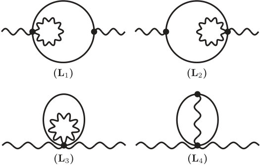 Figure 1
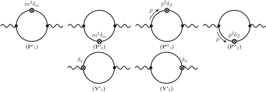 Figure 2
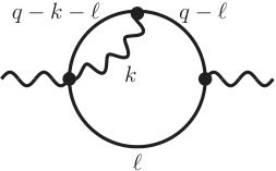 Figure 3
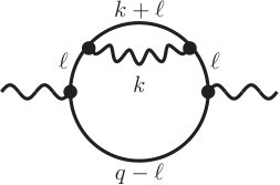 Figure 4
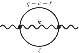 Figure 5
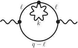 Figure 6
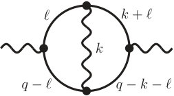 Figure 7
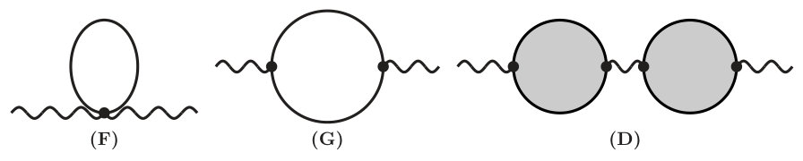 Figure 8
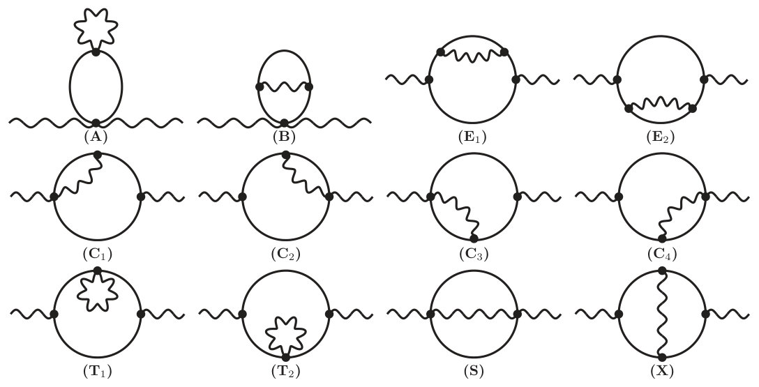 Figure 9
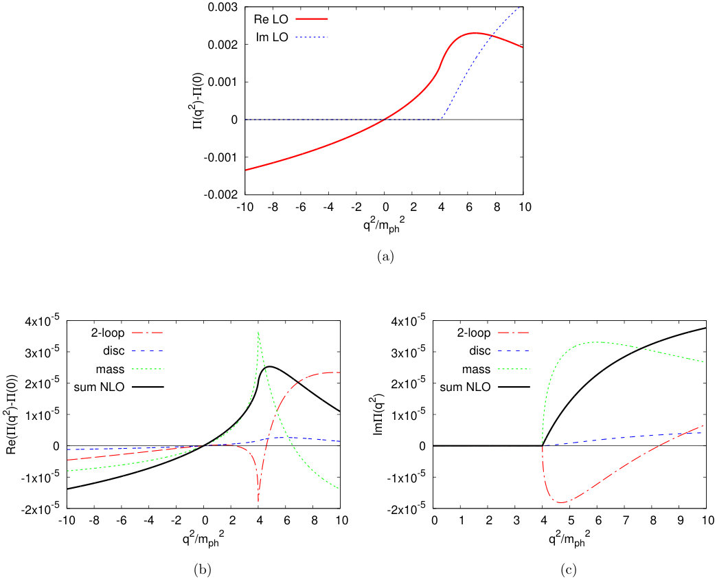 Figure 10
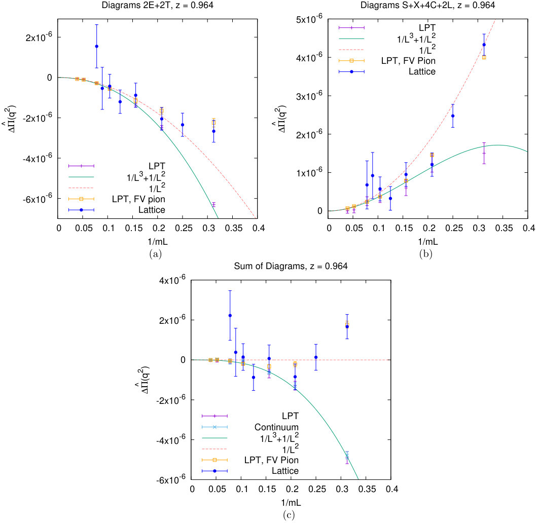 Figure 11
Peer Reviews
No public reviews on file for this paper yet. If you reviewed it on a platform where reviews are public (OpenReview, ICLR, NeurIPS, ICML), you can paste yours below so the community can read it here.
Videos
No videos yet. Explain this paper in a talk, walkthrough, or lecture? Add one.
LU TP 18-30
March 2019
Electromagnetic finite-size effects
to the hadronic vacuum polarization
J. Bijnens
Department of Astronomy and Theoretical Physics,
Lund University, 223 62 Lund, Sweden
J. Harrison
School of Physics and Astronomy, University of Southampton, Southampton SO17 1BJ, United Kingdom
N. Hermansson-Truedsson
Department of Astronomy and Theoretical Physics,
Lund University, 223 62 Lund, Sweden
T. Janowski
School of Physics and Astronomy, University of Edinburgh, Edinburgh EH9 3FD, United Kingdom
A. Jüttner
School of Physics and Astronomy, University of Southampton, Southampton SO17 1BJ, United Kingdom
A. Portelli
School of Physics and Astronomy, University of Edinburgh, Edinburgh EH9 3FD, United Kingdom
Abstract
In order to reduce the current hadronic uncertainties in the theory prediction for the anomalous magnetic moment of the muon, lattice calculations need to reach sub-percent accuracy on the hadronic-vacuum-polarization contribution. This requires the inclusion of electromagnetic corrections. The inclusion of electromagnetic interactions in lattice simulations is known to generate potentially large finite-size effects suppressed only by powers of the inverse spatial extent. In this paper we derive an analytic expression for the finite-volume corrections to the two-pion contribution to the hadronic vacuum polarization at next-to-leading order in the electromagnetic coupling in scalar QED. The leading term is found to be of order where is the spatial extent. A term is absent since the current is neutral and a photon far away thus sees no charge and we show that this result is universal. Our analytical results agree with results from the numerical evaluation of loop integrals as well as simulations of lattice scalar gauge theory with stochastically generated photon fields. In the latter case the agreement is up to exponentially suppressed finite-volume effects. For completeness we also calculate the hadronic vacuum polarization in infinite volume using a basis of 2-loop master integrals.
Contents
I Introduction
One of the most precisely measured quantities in particle physics is the anomalous magnetic moment of the muon , where describes the ratio of couplings of the muon spin and orbital angular momentum to an external magnetic field. Historically, Dirac’s original tree-level prediction was in good agreement with experimental results, but the discrepancy which eventually arose became very strong evidence in support of quantum electrodynamics (QED). Both experimental measurement and Standard-Model predictions for have by now reached a precision of about 0.5ppm where a tension of 3.5-4 is observed (Bennett et al., 2006; Jegerlehner, 2018; Davier et al., 2017; Keshavarzi et al., 2018). Efforts are therefore under way to increase the accuracy of both measurements and theoretical predictions. To address the former two new experiments have been planned, E989 at Fermilab (Logashenko et al., 2015) and E34 at J-PARC (Otani, 2015). The Fermilab experiment is expected to lead to first new results in 2019 and the J-PARC experiment is expected to begin in 2020. Both experiments aim at increasing the experimental accuracy by a factor of 4 to 0.14ppm. To address the latter, we note that the main challenge on the theoretical side comes from non-perturbative contributions, namely the hadronic vacuum polarization (HVP) and hadronic light-by-light scattering (HLbL), of which the HVP constitutes the dominant contribution to the theoretical uncertainty. The traditional approach to estimating the HVP uses dispersion relations together with the optical theorem to relate it to the measured cross section of to hadrons (Davier et al., 2017; Keshavarzi et al., 2018; Davier et al., 2011; Hagiwara et al., 2011). More recently, there has been a significant progress in calculation of the HVP from first principles using lattice QCD (Boyle et al., 2012; Della Morte et al., 2012; Burger et al., 2014; Chakraborty et al., 2014, 2015; Bali and Endrődi, 2015; Chakraborty et al., 2016; Blum et al., 2016a, b; Chakraborty et al., 2017; Della Morte et al., 2017; Borsanyi et al., 2018; Blum et al., 2018; Giusti et al., 2018a; Davies et al., 2019).
Based on simple power counting we expect strong and electromagnetic isospin breaking effects to contribute at the percent level. Given that this corresponds to the level of precision state-of-the-art lattice simulations are able to achieve, these effects need to be included in future calculations. Here we concentrate on electromagnetic effects which can be computed in the lattice-discretized finite-volume theory in several ways. Common to all approaches is the difficulty of defining charged states in a finite volume with periodic boundary conditions and the resulting singularities from photon zero-modes which need to be dealt with. In QEDTL (Duncan et al., 1996, 1997; Borsanyi et al., 2013; Ishikawa et al., 2012; Aoki et al., 2012; de Divitiis et al., 2013; Fodor et al., 2016a) the global zero mode is removed by hand while in QEDL (Hayakawa and Uno, 2008; Davoudi and Savage, 2014; Fodor et al., 2016b; Blum et al., 2007, 2010; Ishikawa et al., 2012; Giusti et al., 2018b, 2017a, 2017b; Blum et al., 2018; Boyle et al., 2017; Lee and Tiburzi, 2016; Matzelle and Tiburzi, 2017; Davoudi et al., 2018) the photon zero-mode is subtracted individually on every time slice. An alternative avenue is to perform simulations with a massive photon (Endres et al., 2016) followed by an extrapolation to zero photon mass to obtain physical results (Endres et al., 2016; Bussone et al., 2018). In yet another approach one introduces charge-conjugation boundary conditions (Polley, 1993; Wiese, 1992; Kronfeld and Wiese, 1993, 1991; Lucini et al., 2016; Hansen et al., 2018) which allow for constructing gauge-invariant charged states in a finite volume. QED corrections have been performed in (Blum et al., 2007, 2010; Borsanyi et al., 2013, 2015; Horsley et al., 2016a, b; Basak et al., 2016; Fodor et al., 2016a; Blum et al., 2018). Isospin-breaking corrections to the HVP have been explicitly considered in (Giusti et al., 2017b; Boyle et al., 2017; Chakraborty et al., 2018a, b; Blum et al., 2018).
A recurring systematic in QCD+QED calculations is the presence of large finite volume (FV) effects, which scale as with the box size for some exponent . This is the result of the photon being a massless particle and the long-ranged nature of electromagnetic interactions. The finite-volume corrections have been studied in effective field theories for the meson masses in (Hayakawa and Uno, 2008; Borsanyi et al., 2015; Davoudi and Savage, 2014; Endres et al., 2016; Lucini et al., 2016; Davoudi et al., 2018) and decay rates in (Lubicz et al., 2017). The finite-volume correction to the HVP at order however has not been previously calculated and this is the subject of this paper. We will extend the methodology for computing finite volume effects described in (Davoudi et al., 2018) to the electromagnetic correction to the HVP.
This paper is organized as follows. section II describes the preliminaries of the HVP function, which are relevant in both finite and infinite volumes. section III describes the analytic derivation of the finite-volume correction of the HVP with electromagnetic correction. This is the main result of this paper. Finally, section IV contains numerical tests of the analytic expressions derived in section III. In appendix A we present a calculation of the NLO HVP in continuum Minkowski space.
II The hadronic vacuum polarization
The main object of interest is the Euclidean 2-point function
[TABLE]
where is a charged or neutral vector current and is the external, Euclidean photon momentum. We start by presenting the calculation for neutral currents relevant for the HVP and then, since the calculation is equivalent up to numerical factors in the summation of diagrams, briefly present the result for charged ones. Note that for neutral currents Ward-Takahashi identities imply that . The quantity is ultraviolet divergent and it is conventional to calculate the finite, subtracted quantity
[TABLE]
This may be expanded in powers of the electric charge as , where and are the leading order (LO) and next-to leading order (NLO) terms, i.e. and , respectively.
Although the two-pion contribution to the HVP is small compared to the vector resonance one, it is the lightest contribution and dominates finite-volume effects (Aubin et al., 2016). Here we consider the electromagnetic corrections to this contribution, and use scalar QED as an effective theory of elementary pions. The scalar QED Lagrangian in Euclidean space is given by
[TABLE]
for a scalar field , a photon field and the electromagnetic tensor . We only consider the leading order scalar interactions, higher-order contributions, where is the four-scalar vertex coupling, enter at three loop order. The connected diagrams needed at NLO for the HVP are therefore those in fig. 1. Seeing that some of these diagrams are equal up to relabelling of momenta in the loops, we only need to calculate seven topologies, namely (A), (B), (E1), (C1), (T1), (S) and (X). Diagrams (A) and (B) do not depend on the external momentum and thus cancel in the subtraction, so only (E), (C), (T), (S) and (X) contribute. The topology subscripts have here been suppressed and will remain so in the rest of the paper. The labelling refers to embedded sunrise (E), contact (C), embedded tadpole (T), sunset (S) and photon exchange (X). It should be noted that also the diagrams in (D) in fig. 2 are in general needed at NLO, but they are excluded for in and are in infinite volume simply related to the square of the LO contribution, given by diagrams (F) and (G), as will be discussed in more detail later. The specific choice of the photon rest frame is elaborated on in section III.
For completeness, we also calculated the NLO HVP in infinite volume. We considered both a Euclidean lattice using lattice perturbation theory, as well as continuum Minkowski space. The Minkowski space calculation is presented in appendix A.
Using the Feynman rules from the continuum Euclidean space Lagrangian yields the momentum-space integrands of the diagrams
[TABLE]
where is the photon loop momentum, is the pion-loop momentum and is the number of dimensions. Similar expressions for Minkowski space are given in section A.1.
III Finite-size effects to the scalar vacuum polarization
We can express the renormalized HVP function through the following trace of the subtracted vector two-point function
[TABLE]
where the photon rest frame has been specifically chosen. There are two main reasons for choosing this frame. First and foremost, this is typically the frame used in current lattice calculations. Moreover, it simplifies the finite-volume calculation immensely, in particular as the coefficients defined below then are independent of the photon momentum.
Note that diagrams (A) and (B) automatically vanish in the subtraction in eq. 13, as they are independent of the external momentum. Moreover, the disconnected contribution (D) is zero in because the photon propagator vanishes in the rest frame. We are thus left with diagrams (E), (C), (T), (S) and (X), so that, including all permutations of the diagrams, the contribution to the HVP can be written as
[TABLE]
where denotes the contribution from diagram (U). Next we define the corresponding integrand (excluding the factors of in the measure) as .
In finite-volume, we assume space to be periodic with spatial extent and time to remain infinite. We now present the procedure followed to determine the finite-size effects to which decay like powers of . This strategy is a direct generalization of the procedure for one-loop integrals in Ref. (Davoudi et al., 2018). The remaining part of this section is a formal description of our approach to compute the large volume expansion. Although the final result presented in section III.1 is quite compact, intermediate expressions can be quite cumbersome. It is therefore desirable to implement the whole strategy in a computer algebra system. The calculations presented here were performed using FORM (Vermaseren, 2000) and Mathematica (Inc., ), and the associated Mathematica notebook is provided as a supplement of this paper under the General Public License version 3. Intermediate products of the derivation are provided for future reference in appendix D.
For a given diagram, we start by computing the two energy integrals in and using contour integration. Feynman integrands are rational functions and this integration is systematically feasible analytically. We thus obtain
[TABLE]
In analogy with eq. 13, we also define the subtracted quantities . The finite volume effects on for diagram (U) in can then be written as
[TABLE]
where finite-volume sums are on quantized momenta of the form with a vector with integer components, and a primed sum means that the origin is excluded, which here comes from the prescription. One important aspect here is that we are only considering the case. This means that pions in diagrams are purely virtual and cannot generate power-like finite-volume effects through on-shell singularities. Using the Poisson summation formula for the pion part yields
[TABLE]
where the omitted terms denoted by ellipsis are the exponentially suppressed contributions from the virtual pions.
To determine power-like finite-size effects in the five diagrams (E), (C), (T), (S) and (X), we closely follow the strategy laid out in Davoudi et al. (2018). One starts by isolating the singularities in the photon momentum in ,
[TABLE]
where is an integer that depends on the diagram in question, , and is an analytic function in the norm such that . The analytical structure of all five diagrams is such that . If we now substitute and expand in , the finite volume effects for diagram can be written as a power series in (up to exponentially small corrections),
[TABLE]
The coefficients are given by
[TABLE]
where is, as in Ref. (Davoudi et al., 2018), the sum-integral difference operator
[TABLE]
Although is an analytic function in the norm , the norm itself in not analytic in the components of at the origin, which generates the effects in eq. 19. We will now present the full expressions for the finite-size effects to each of the five diagram topologies (S), (T), (C), (E) and (X).
III.1 The full finite-size effects
To find the finite-size effect to a diagram (U), the last step to perform is the calculation of the coefficients in eq. 20. For the specific kinematics chosen here, i.e., spatial momenta equal to zero (cf. eq. 13), the integrand is independent of the photon momentum direction . The function then has the form
[TABLE]
where identically to Ref. (Davoudi et al., 2018), we define the coefficients . These can be calculated numerically in several ways, and one possibility is presented in (Davoudi et al., 2018). The first three coefficients are , and .
The functions in eq. 22 can be written as linear combinations of integrals of the form
[TABLE]
where , and
[TABLE]
They arise after integrating the angular dependence of the integrals over momentum for which . There are several useful recursion relations and properties for these integrals, which we summarise in appendix B. For instance, for in , it is possible to write any as a linear combination of the six simple functions , , , , and as well as their respective derivatives. The complete list of expressions that lead to these integrals, in particular, the expansion eq. 18, are given explicitly for all diagram topologies in appendix D.
Finally, we summarize here the final expressions for the finite-volume effects to each diagram, where every term implicitly depends on
[TABLE]
and where all the expressions are given up to corrections. We can sum these terms according to eq. 14. The resulting series in for the HVP at NLO is
[TABLE]
where one notices the important cancellation of the terms. This result can be understood from the underlying physics since the current is neutral and a photon far away thus sees no charge. This cancellation has potentially important consequences regarding the prediction of the contribution from the HVP to using lattice simulations. Indeed, for typical physical simulations with , one has . Under the safe assumption that the QED corrections to are , the electromagnetic finite-size effects discussed here would represent a contribution smaller than , well below the level required to reduce by a factor of the current theoretical uncertainties on . Finally, for one has , which means that in this regime the new, power-like finite-size corrections introduced by QED are in principle not dominant compared to the exponential QCD effects. In the following sections, we demonstrate that this cancellation does not occur for charged currents, and that it is universal in full QCD+QED and therefore directly applicable to lattice results.
III.2 Charged currents
For the neutral currents only charged pions are considered. If also is included, the current in eq. 1 can be charged and the current-current correlator can therefore be rewritten as
[TABLE]
for two functions and that are equal for neutral currents. We are again interested in the case and calculate the subtracted quantity
[TABLE]
The function can be expanded in the electromagnetic coupling just as before, and we here denote the NLO contribution by . The possible topologies of the NLO diagrams are the same also here, but having charged currents implies that some of them may be forbidden and the overall numerical factors can be different compared to the netural case for those that are not. In order to find these differences, we include the neutral pion by defining the meson matrix and the current matrix as
[TABLE]
The covariant derivative of can then be put in the form
[TABLE]
and the kinetic part of the Lagrangian is given by
[TABLE]
Using this, we find that diagram (X), one of the permutations of diagram (T), two of the permutations of (C) and one of the permutations of diagram (E) are forbidden. Moreover, the overall numerical factors change such that the relevant NLO contribution becomes
[TABLE]
This yields the NLO FV effects as
[TABLE]
up to corrections. The part does not vanish here. This is expected, since the current no longer is neutral and the physical argument used for the neutral case no longer applies.
III.3 Universality of the finite-size corrections
In the above we showed that in one-loop scalar QED the leading contribution to the FV effects on the subtracted vacuum polarization function is of order in . We will now show that this conclusion is independent of the effective-field-theory formulation chosen for the finite volume calculation.
The corrections to the current-current correlator , which we denote , can be written as
[TABLE]
where the symbol is an abbreviation for the integration over the space-time positions , , and . This amplitude is identical to the amputated light-by-light scattering Green’s function with two legs contracted with the photon propagator. We will argue below that the light-by-light matrix element at our choice of kinematics is free of singularities and therefore expected to have only exponential finite volume corrections. As a consequence, the only source of power-like corrections will necessarily have to come from the photon propagator pole.
A useful form-factor decomposition of the light-by-light amplitude with form factors that are free of kinematic singularities is given in equation (3.14) of (Colangelo et al., 2015). We note that all tensor structures have at least one factor of each of the , , and . In our formula, we need to replace two of those external momenta with and the remaining two with and , respectively. Therefore all the tensor structures will be proportional to either or for some Lorentz indices and , which in turn can be replaced with using the –dimensional integral (or sum in FV) formula:
[TABLE]
This means that each of the tensor structures contribute a factor of , which cancels the pole in the photon propagator. Since the light-by-light form factors are free of kinematic singularities, and we work with Euclidean momenta which cannot give rise to any on-shell singularities, they do not have any poles in . This means that the leading FV correction will come from a term which is constant in , which has the contribution proportional to , completing the proof.
The above argument can be simplified by considering the scalar HVP form factor
[TABLE]
The function then has the form
[TABLE]
where the kernel satisfies the Ward identities . The kernel function is a momentum space amplitude and any singularities must correspond to physical states. In Euclidean space with external momenta being real, the function can not have any poles corresponding to physical states, which would have to satisfy where is the momentum going through any cut in the diagram. We can decompose in a series of tensor structures multiplying form factors, which can generally be written as
[TABLE]
Since is free of singularities and the tensor structures are linearly independent, the form factors must be free of singularities as well. The Ward identities impose a relation on the form factors simplifying the expression to
[TABLE]
As noted before, the form factors and are free of singularities, however must have a zero at to cancel the pole originating from the tensor structure it is multiplying. We conclude that must be proportional to . Finally, the form factor decomposition of consistent with Lorentz symmetry, parity, and Ward identities is
[TABLE]
As before, we note that the form factors and do not have poles in and the tensor structure has two factors of which become under the integral, which cancels the photon propagator pole. As before, this results in the leading contribution to the FV correction to be proportional to .
IV Numerical validation
In this section we provide two different numerical checks of the finite-volume corrections derived in section III.1. Scalar QED is ideally suited for numerical simulations. Indeed, as we will now explain in detail, the theory can be written on a discrete space-time simply by replacing derivatives with finite differences. In the two following subsections, we describe two different Monte-Carlo strategies to compute the volume dependence of the scalar vacuum polarization. Firstly, the master formula eq. 17 is evaluated directly using a Monte-Carlo integrator. Secondly, the finite-volume vacuum polarization is calculated at using lattice -scalar-QED simulations, following the strategy described in (Davoudi et al., 2018). Finally, we discuss the comparison of these results with analytical predictions.
IV.1 Scalar QED on a lattice
In this section we explain our definition of the lattice discretized theory. The conventions and notations are identical to (Davoudi et al., 2018). We consider space-time to be an Euclidean four-dimensional lattice with spatial extent , time extent , and lattice spacing . Lattice QED is then defined by the action
[TABLE]
with scalar and gauge actions
[TABLE]
respectively, with . The summation is over all the sites of the lattice. The covariant derivative is defined in terms of the gauge link , where is the electric charge of the scalar particle, as
[TABLE]
We also introduce the forward derivative , which appears in the Feynman gauge-fixing term. The electromagnetic tensor is defined as
[TABLE]
Expectation values in this theory are expressed in terms of the path integral
[TABLE]
where the integral measures represent integrations over the field variable at each lattice site. The subscript L indicates that we are working within the QEDL prescription where the spatial zero mode is set to zero on each time slice,
[TABLE]
Below we will expand the path integral to NLO in . To this end it is instructive to first integrate out the scalar fields analytically,
[TABLE]
where represents the observable after the Wick contraction. The action is symmetric under and therefore, contributions odd in do not contribute to expectation values. To NLO we can therefore set .
We rewrite the operator with the help of the translation operator , as
[TABLE]
The expansion of in the electric charge takes the form,
[TABLE]
where
[TABLE]
Inserting the kernel expanded in into the scalar-QED action,
[TABLE]
allows us to identify the Feynman rules for the inverse free propagator, the scalar-photon-vertex and the scalar tadpole, respectively. In particular, the scalar propagator in the background field is then readily given by
[TABLE]
From this expansion it is a simple exercise to derive the associated Feynman rules for lattice perturbation theory.
IV.2 Lattice perturbation theory Monte-Carlo strategy
In order to numerically check the analytic results we numerically calculate the finite-size corrections for each diagram in scalar QED using lattice perturbation theory (LPT). We present below the analytic expressions for the diagrams (E), (C), (T), (S), and (X) in lattice perturbation theory, which are the discrete version of eqs. 8, 9, 10, 11 and 12.
[TABLE]
where .
On the lattice, there is potentially an infinity of new scalar-photon vertices because of the compactification of the gauge field in eq. 48. These vertices are classically discretisation effects, but at the quantum level they can generate finite contributions when multiplying power divergences, and ignoring them can potentially break Ward-Takahashi identities. If one consistently keeps contributions which do not vanish in the continuum limit, four new diagrams appear in lattice perturbation theory, represented in fig. 3. Both diagrams (L3) and (L4) are independent of the external momentum and therefore vanish in the subtracted vacuum polarization function eq. 13.
The integrand for diagrams (L1) and (L2) is given by
[TABLE]
We integrate these expressions using the VEGAS algorithm (Lepage, 1978), and more specifically its C++ implementation in the Cuba library (Hahn, 2005). This integration algorithm builds upon Monte Carlo techniques and creates histograms approximating the shape of the function which are then used as probability distributions for importance sampling. This is particularly useful for the integrals considered here, which are eight-dimensional, and have a complicated sawtooth-like structure, as we discuss now. In finite volume, the lattice momentum is discretized and the corresponding sums can be dealt with in VEGAS by realising that for a function
[TABLE]
where is the floor operator rounding down to the nearest integer. This is extendable to any number of dimensions. As for the analytic results, we assume an infinite time extent and pions are in infinite volume, cf. eq. 17, so that only three of the eight integrals are sums in the finite-volume calculation. The implementation of the calculation is distributed as a C++ source code under the General Public License v3 in the supplementary material of this paper, and it features an option to also have the pions in a finite volume as instructed in the comments. This is particularly useful when comparing to lattice data, as discussed later.
Each diagram depends on the lattice spacing . We introduce a scaling parameter such that the lattice spacing is varied according to and calculate the diagrams for four different values of , namely , from which a continuum extrapolation is made by fitting against some polynomial in . We find, using a pion mass such that , that the dependence is mild. We find the best description of the data in terms of a leading correction, as expected from the symmetry of scalar QED.
Rewriting the sums as in eq. 64 yields sawtooth-like behavior since the integrands of the finite-size effects then are of the form . The number of discontinuities in this function is on the order of (or if also the pions are put in finite volume) which means that it can be hard to sample the integrand efficiently and thus get reliable values and errors from Cuba. The reliability can be checked by comparing the results from calculations with a varying number of Monte Carlo evaluation points for a certain . We find that using points gives reliable results for . Our result are summarized at the end of this section.
IV.3 Lattice scalar QED simulations
An alternative avenue which we also explore is to evalute the lattice-discretized path integral in eq. 52 by means of a Monte Carlo integration for a series of different spatial extents . This allows for mapping out the volume dependence, thereby checking our analytical predictions. Instead of numerically solving the momentum sums as in the previous section one directly samples the path integral in eq. 52. In particular, we compute the vacuum polarization tensor as the discrete Fourier transform of the two-point function
[TABLE]
with the lattice conserved vector current
[TABLE]
After carrying out the Wick contractions we can write the expression for the vacuum polarization tensor in terms of the propagator in eq. 57 acting on a point source ,
[TABLE]
where the expectation value represents the functional integration on the gauge potential . We evaluate this correlation function numerically using a setup identical to the one in (Davoudi et al., 2018), in fact the data used here are a side-product of the calculation presented in this previous work. The covariant Klein-Gordon equation is solved in a stochastic background field to form the interacting scalar propagator . Using the expansion eq. 57, this can be achieved using the fast Fourier transform algorithm. As a consequence, this method has a reasonable numerical cost, which is independent from the chosen scalar mass and has a quasilinear complexity in the number of lattice points. We refer the reader to (Davoudi et al., 2018) for more details on the computational aspects.
In principle, the full correction to the scalar vacuum polarization also receives contributions from the diagrams in fig. 4, coming from the 1-loop counter-terms of scalar QED. We assume that these counterterms are determined through a set of renormalization conditions in infinite volume, and therefore are independent of the volume. Because these diagrams do not contain photon propagators, they clearly do not contribute to eq. 17. However, the same formula assumes scalar particles to be in infinite-volume, which is not the case in the lattice simulation. Although these finite-volume corrections are exponentially suppressed, they can be greatly enhanced by the ultraviolet-divergent values of the counter-terms. We therefore included these diagrams to ensure that exponential finite-volume corrections are negligible for reasonably large values of (the typical threshold for lattice QCD simulations is ). The details of the renormalisation prescription used here are given in appendix C. The cost of computing the extra counter-term diagrams is negligible, since they do not depend on the gauge field.
IV.4 Numerical results
In fig. 5 we compare the analytic results to LPT and lattice data. We use and , i.e. . The red dashed line is the term and the green solid line is the full expression of the form in the corresponding analytic expression in section III.1. The purple points are the infinite volume pion LPT points for a finite , and the crossed blue points are the continuum extrapolated values. The orange box shaped points are finite volume pion LPT data. From the infinite volume pion LPT data we clearly see that the full analytic form is much better than when including only the term and the agreement is excellent up to for all diagrams. Other values of yield a similar level of agreement. We see that the lattice data starts to deviate from the analytic curve after , but the finite volume pion calculation reproduces precisely this behavior. We thus attribute the discrepancies to the exponential finite-size effects that are neglected in eq. 17 for the analytic calculation as well as in the infinite volume pion LPT Monte-Carlo. Moreover, for we found that the difference between the infinite-volume pion and finite-volume pion data is on the order of , an order of magnitude smaller than the naive suppression from a factor of between the LO and the NLO HVP, viz. .
V Conclusions
We have performed a 2-loop calculation of the corrections to the hadronic vacuum polarization in scalar QED. We presented the infinite volume results in terms of 2-loop master integrals from which we obtained an analytic expression for the finite volume correction to the HVP at this order. We found that even though each of the individual diagrams contributes as , these terms all cancel when combined. We argued that this cancellation is expected on physical grounds for neutral currents and show that it does not occur for charged currents. We also argued that this cancellation is universal, i.e., it occurs regardless of the effective theory used to derive this result.
All our results were tested numerically using two different approaches - direct integration of lattice perturbation theory integrals using VEGAS and lattice scalar U(1) gauge theory with stochastically generated photon fields. We find good agreement between analytic results and results from both numerical approaches. While absent from our analytical expressions, exponentially suppressed finite volume effects are visible in our results from the lattice simulation
Finally, an important consequence of this work is that for the foreseeable future finite-volume effects on the QED corrections to the hadronic vacuum polarization are likely to be negligible in lattice simulations. For instance, we expect this to hold even if lattice computations aimed at matching experimental projections of a four-fold reduction in the error on by Fermilab (Logashenko et al., 2015) and J-PARC (Otani, 2015) down to 0.14ppm. This assumes a typical lattice simulation where the pion mass times the spatial extent is larger than four, for which this work estimates the finite-size effects to be at the level of only a few percent of the correction to the HVP function . Unless these effects come with an unnaturally large coefficient in the full theory, they should be negligible compared to the per-mil accuracy required on the HVP contribution to . Of course, large coefficients cannot be excluded considering how critical it is to properly estimate the theoretical uncertainty on , particularly in the perspective of confirming or excluding the current discrepancy between experiment and theory on this quantity. The results of this work together with simulations of full lattice QCD+QED even with a limited number of volumes, should allow to constrain the size of these effects.
Acknowledgements.
A.P. would like to thank the High Energy Physics Group of Lund University for its warm welcome, important parts of this work were initiated during A.P.’s visit in Lund. Lattice computations presented in this work have been performed on DiRAC equipment which is part of the UK National E-Infrastructure, and on the IRIDIS High Performance Computing Facility at the University of Southampton. T.J. and A.P. are supported in part by UK STFC grants ST/L000458/1 and ST/P000630/1. A.P. also received funding from the European Research Council (ERC) under the European Union’s Horizon 2020 research and innovation programme under grant agreement No 757646. J.B. and N.H.T. are supported in part by the Swedish Research Council grants contract numbers 2015-04089 and 2016-05996, and by the European Research Council (ERC) under the European Union’s Horizon 2020 research and innovation programme under grant agreement No 668679. J.H. was supported by the EPSRC Centre for Doctoral Training in Next Generation Computational Modelling grant EP/L015382/1. A.J. received funding from STFC consolidated grant ST/P000711/1 and from the European Research Council under the European Union’s Seventh Framework Program (FP7/2007- 2013) / ERC Grant agreement 279757.
Appendix A In continuous infinite volume
In this section the HVP is considered in continuous infinite volume Minkowski space. We calculate and in and numerically compare their respective sizes. The corresponding calculation in QED can be found in (Kallen and Sabry, 1955; Barbieri and Remiddi, 1973).
In Minkowski space the scalar QED Lagrangian is
[TABLE]
The relevant counterterms for the parameters above, are defined in the counterterm Lagrangian
[TABLE]
In dimensions these are given by
[TABLE]
Note that diagrams (A) and (T) identically vanish in dimensional regularization, so that we are left with diagrams (F), (G), (D), (B), (E), (C), (S) and (X). The two HVP contributions can thus be written (cf. the FV case in eq. 14)
[TABLE]
Using the tensor structure of and the Ward identity it is easy to see that the disconnected part is given by the squared LO contribution, . The diagrams are given in section A.1.
Using Lorentz invariance identities and integration by parts, the 2-loop integrals can be rewritten in a basis of master integrals. The program Reduze2 (von Manteuffel and Studerus, 2012) employs a Laporta algorithm in order to do this, and allows the user to define such a basis. The master integrals used here are the subtracted parts of
[TABLE]
All but integral are divergent and thus require expansion in in order to isolate the divergent parts from the finite ones, something which can be done in both Euclidean and Minkowski space. For a Euclidean spacetime the analytic results can be found in (Martin, 2003). However, working in Minkowski space, the corresponding expressions are here given in section A.2.
Note that in the threshold shift can, and does, induce a sign change of the imaginary part of at some . However, this does not occur for an on-shell scheme or with the physical mass. The physical mass is related to through
[TABLE]
The HVP can therefore also be expanded around this mass,
[TABLE]
where in the last step the disconnected part was separated from the NLO contribution. To simplify the expressions, let us further define
[TABLE]
The HVP contributions at LO and NLO are thus
[TABLE]
where the quantities with bars are the finite parts of the integrals in appendix A. These contributions as well as the corresponding subtracted quantities are plotted in fig. 6 for MeV, MeV and . As can be seen, the NLO parts are roughly two orders of magnitude smaller than LO, this is due to the additional power of . Moreover, it can be noted that on average is significantly smaller than the other parts, and that and combine to give the proper non-singular threshold behavior.
A.1 Diagrams in Minkowski space
Using the Feynman rules for the Lagrangian in eq. 68, the diagrams are
[TABLE]
A.2 Master integrals
Below, each Minkowski-space master integral in appendix A has been separated into a finite and an infinite part, the finite one denoted by a bar. The analytic expressions for these finite integrals are given in (Martin, 2003), and are in terms of Riemann zeta functions as well as the polylogarithm functions and ,
[TABLE]
Appendix B The scalar loop integrals
Consider the dimensionless function given by
[TABLE]
where
[TABLE]
This function converges if and only if . The relations between , the external momentum , the integration variable and the variable are and . It is also possible to write explicitly in terms of hypergeometric functions as
[TABLE]
where is the hypergeometric function defined by
[TABLE]
However, the form eq. 80 is complex and might not be the most useful in practice. The functions are actually related to each other and can be expressed as combinations of a smaller set of functions. One starts by noticing the relations
[TABLE]
The identity eq. 82 directly implies that
[TABLE]
i.e. the index is decreased by taking derivatives in . One can further note that
[TABLE]
which is easily proven by multiplying and dividing the integrand a factor . For the case it is possible to find a recursion relation by using eq. 83, this by partially integrating the definition of :
[TABLE]
where in the last step the convergence requirement as well as eq. 83 were used. By writing x^{4}=x^{2}\Big{(}x^{2}+1\Big{)}-x^{2} one then finds the relation
[TABLE]
or, for ,
[TABLE]
Inspired by the recursion relation in eq. 84, define for the functions
[TABLE]
Now, using eq. 84 for and an integer
[TABLE]
The second identity eq. 83, combined with an integration by parts of eqs. 79 and 84 leads to
[TABLE]
where we used the prime notation for derivatives in . Using this last relation and eq. 89, it is clear that for any positive integer couple such that , is a linear combination of the six following functions and their derivatives
[TABLE]
Appendix C Lattice scalar QED renormalisation scheme
We start by rewriting the Lagrangian of scalar QED in term of the renormalized fields and parameters defined by , , , , where a subscript 0 denotes a bare quantity. The counterterm part of the lattice Lagrangian is given by
[TABLE]
At the order relevant here, the electric charge does not renormalize, i.e. . The discretized action is gauge invariant and, as it is well known in the continuum, the theory can be renormalized by removing divergences in the self-energy function and by using as imposed by the Ward-Takahashi identities. By denoting the self-energy function at momentum , we choose the following renormalization prescription
[TABLE]
with where is the time extent of the lattice. This prescription allows to compute the wave function renormalization at finite time extent. In all the finite-time numerical results presented in this paper we used . For , this prescription gives back the more traditional conditions, where one assumes that the self-energy and its derivative vanishes at . For and we found
[TABLE]
Appendix D Explicit forms of energy-integrated diagrams
The subtracted functions can be written in the form
[TABLE]
where , and are functions of , and . The above factorization is chosen such that the dependence on in these functions is different from pure powers of . This means that they can depend on in denominators through the energy (which often shows up in denominators) as well as the combination for the velocity and the unit vector . This separation is useful since, for a given , a large volume expansion of , which multiplies , has leading power behavior of order . It is therefore only the term in the sum over which can give a contribution to and thus a finite-size correction, where the coefficients and are defined through
[TABLE]
Defining the velocity is particularly useful as any term with such a factor vanishes when integrating over . The velocities can enter also in the small expansion, for instance through
[TABLE]
In this appendix, we list the non-vanishing functions , , and separately for each diagram (U).
D.1 Diagram (S)
First consider (S), whose integrand for the momentum assignment in fig. 7 is
[TABLE]
The non-vanishing functions entering and are
[TABLE]
D.2 Diagram (T)
Now consider the calculation of diagram (T) with momenta as in fig. 8. The integrand is
[TABLE]
The non-vanishing functions here are
[TABLE]
Note that since cannot be expanded in small . Also, since we cannot have any contributions of order .
D.3 Diagram (C)
For diagram (C) with momenta as in fig. 9, the integrand is
[TABLE]
This gives
[TABLE]
D.4 Diagram (E)
The integrand for diagram (E), with the momentum assignment in fig. 10, is
[TABLE]
Here we have
[TABLE]
D.5 Diagram (X)
Assigning momenta as in fig. 11, the integrand of diagram (X) is
[TABLE]
The non-vanishing functions are now
[TABLE]
The reference list from the paper itself. Each links out to its DOI / PubMed record.
- 1Bennett et al. (2006) G. W. Bennett et al. (Muon g-2), Phys. Rev. D 73 , 072003 (2006) , ar Xiv:hep-ex/0602035 [hep-ex] . · doi ↗
- 2Jegerlehner (2018) F. Jegerlehner, Proceedings, KLOE-2 Workshop on e + e − superscript 𝑒 superscript 𝑒 e^{+}e^{-} Collision Physics at 1 Ge V: Frascati, Italy, October 26-28, 2016 , EPJ Web Conf. 166 , 00022 (2018) , ar Xiv:1705.00263 [hep-ph] . · doi ↗
- 3Davier et al. (2017) M. Davier, A. Hoecker, B. Malaescu, and Z. Zhang, Eur. Phys. J. C 77 , 827 (2017) , ar Xiv:1706.09436 [hep-ph] . · doi ↗
- 4Keshavarzi et al. (2018) A. Keshavarzi, D. Nomura, and T. Teubner, Phys. Rev. D 97 , 114025 (2018) , ar Xiv:1802.02995 [hep-ph] . · doi ↗
- 5Logashenko et al. (2015) I. Logashenko et al. (Muon g-2), Fundamental constants 2015: Fundamental constants 2015 Eltville, Germany, February 1-6, 2015 , J. Phys. Chem. Ref. Data 44 , 031211 (2015) . · doi ↗
- 6Otani (2015) M. Otani (E 34), Proceedings, 2nd International Symposium on Science at J-PARC: Unlocking the Mysteries of Life, Matter and the Universe (J-PARC 2014): Tsukuba, Japan, July 12-15, 2014 , JPS Conf. Proc. 8 , 025010 (2015) . · doi ↗
- 7Davier et al. (2011) M. Davier, A. Hoecker, B. Malaescu, and Z. Zhang, Eur. Phys. J. C 71 , 1515 (2011) , [Erratum: Eur. Phys. J.C 72,1874(2012)], ar Xiv:1010.4180 [hep-ph] . · doi ↗
- 8Hagiwara et al. (2011) K. Hagiwara, R. Liao, A. D. Martin, D. Nomura, and T. Teubner, J. Phys. G 38 , 085003 (2011) , ar Xiv:1105.3149 [hep-ph] . · doi ↗