Self-consistent-field ensembles of disordered Hamiltonians: Efficient solver and application to superconducting films
Matthias Stosiek, Bruno Lang, Ferdinand Evers

TL;DR
This paper introduces an efficient parallelized solver for self-consistent-field theories of disordered fermions, applied to superconducting films, revealing new physical phenomena and validating the importance of full self-consistency in such models.
Contribution
It presents a novel, scalable kernel-polynomial based solver for self-consistent disordered Hamiltonians, enabling large-scale simulations and insights into superconducting phenomena.
Findings
Non-monotonic coherence length behavior with disorder
Formation of superconducting islands at large scales
Partial self-consistency schemes may miss key physics
Abstract
Our general interest is in self-consistent-field (scf) theories of disordered fermions. They generate physically relevant sub-ensembles ("scf-ensembles") within a given Altland-Zirnbauer class. We are motivated to investigate such ensembles (i) by the possibility to discover new fixed points due to (long-range) interactions; (ii) by analytical scf-theories that rely on partial self-consistency approximations awaiting a numerical validation; (iii) by the overall importance of scf-theories for the understanding of complex interaction-mediated phenomena in terms of effective single-particle pictures. In this paper we present an efficient, parallelized implementation solving scf-problems with spatially local fields by applying a kernel-polynomial approach. Our first application is the Boguliubov-deGennes (BdG) theory of the attractive- Hubbard model in the presence of on-site disorder;…
Click any figure to enlarge with its caption.
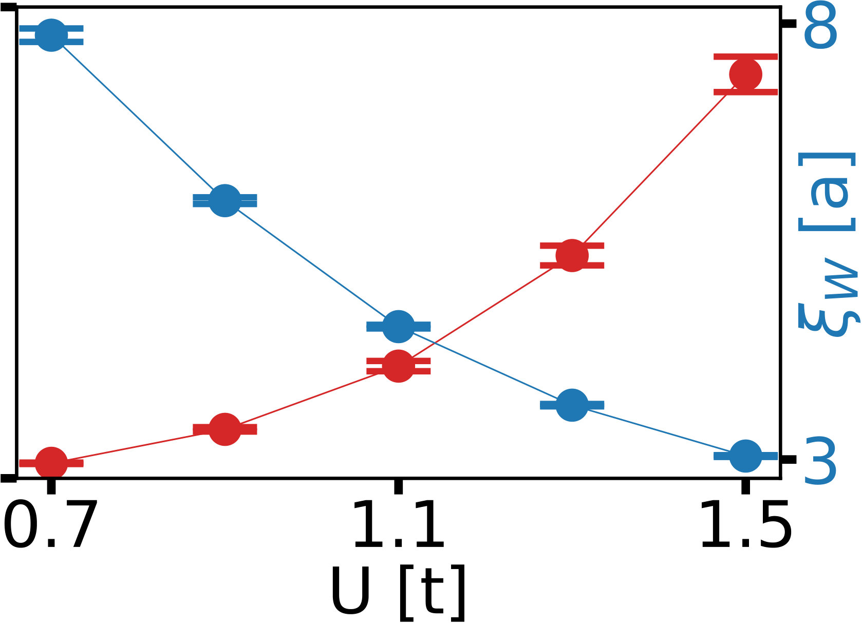 Figure 1
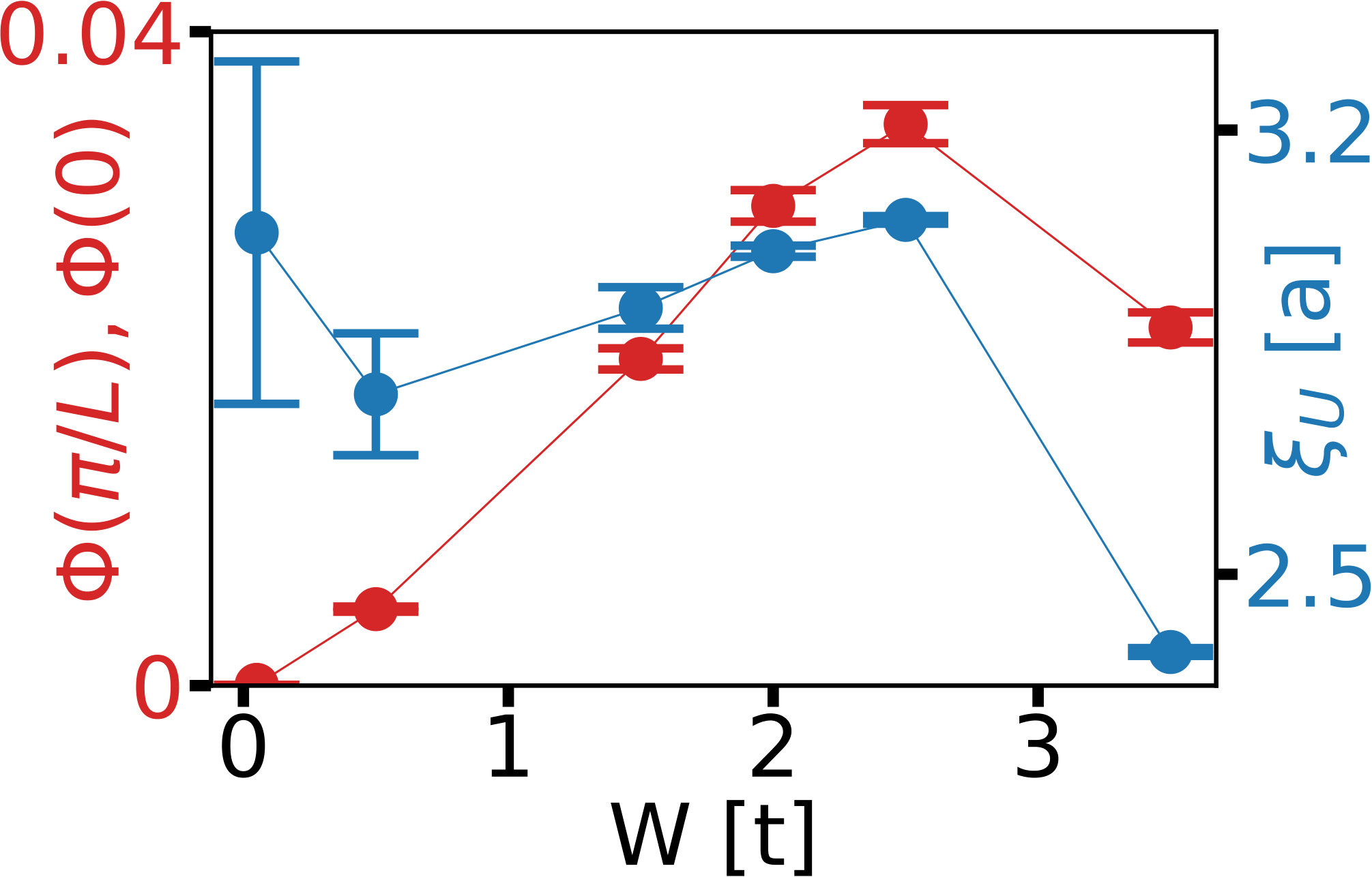 Figure 2
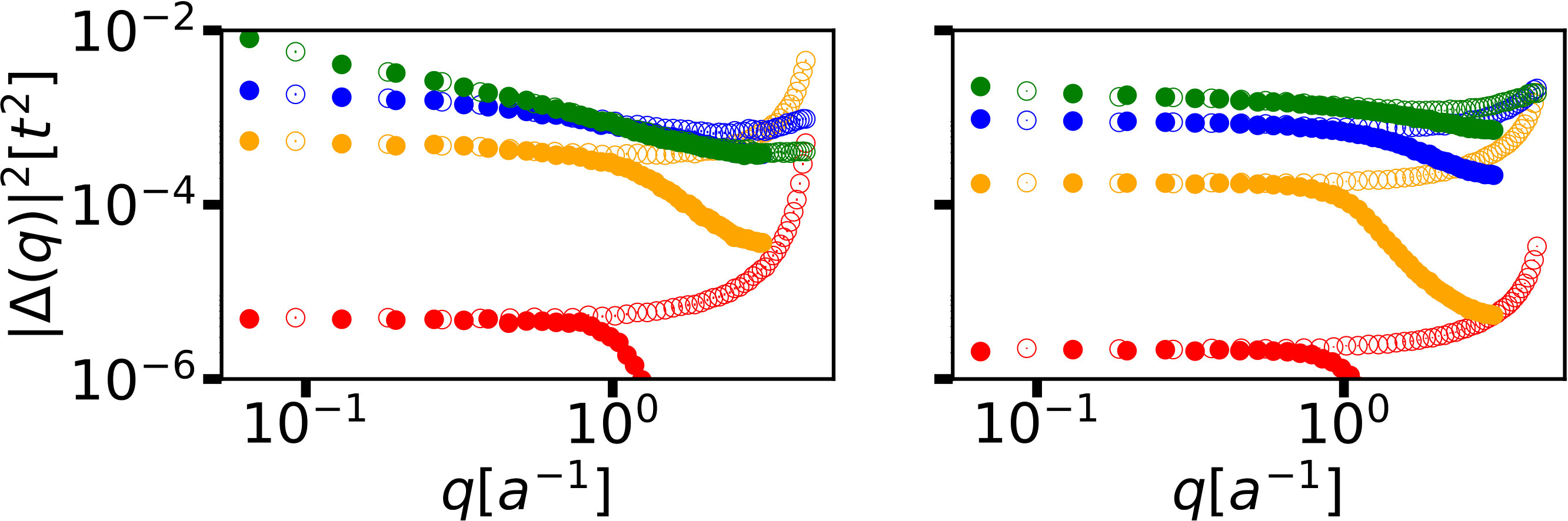 Figure 3
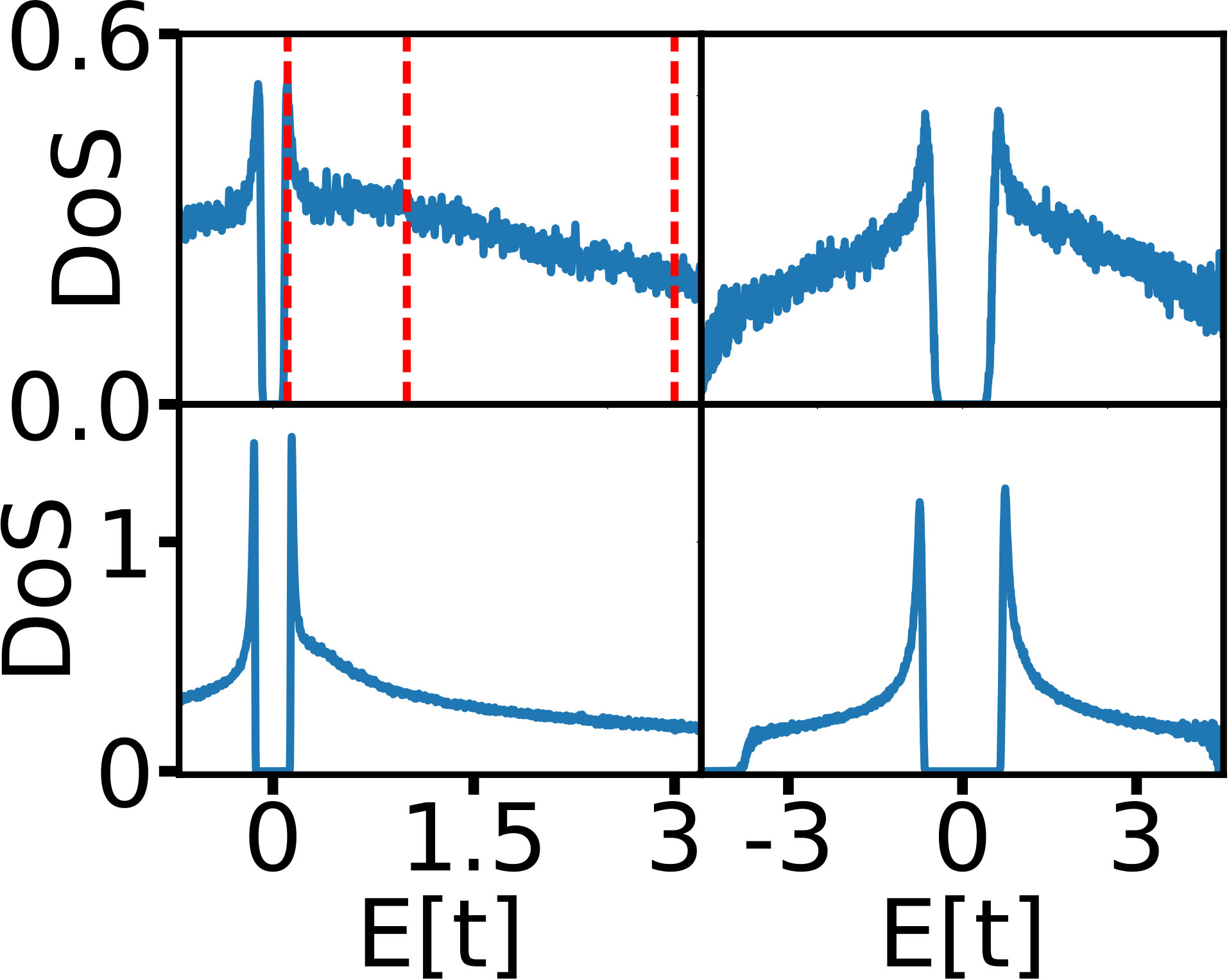 Figure 4
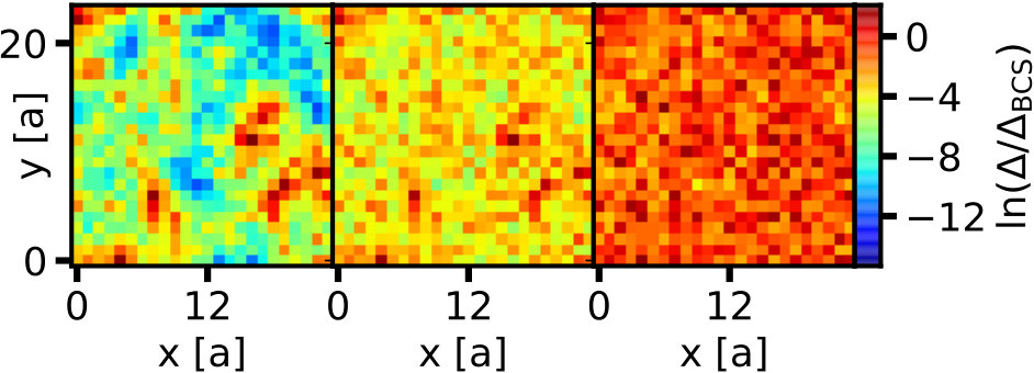 Figure 5
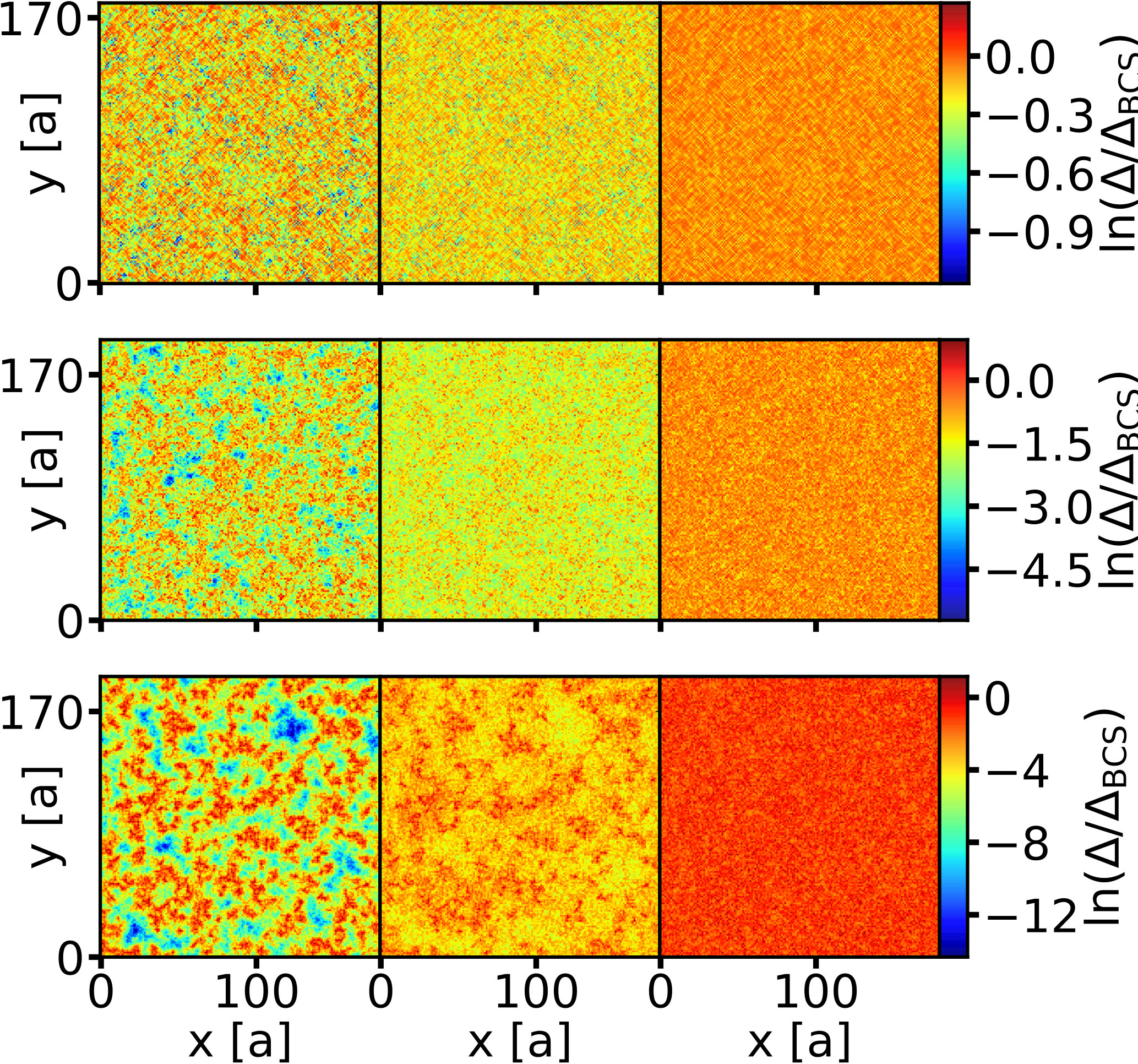 Figure 6
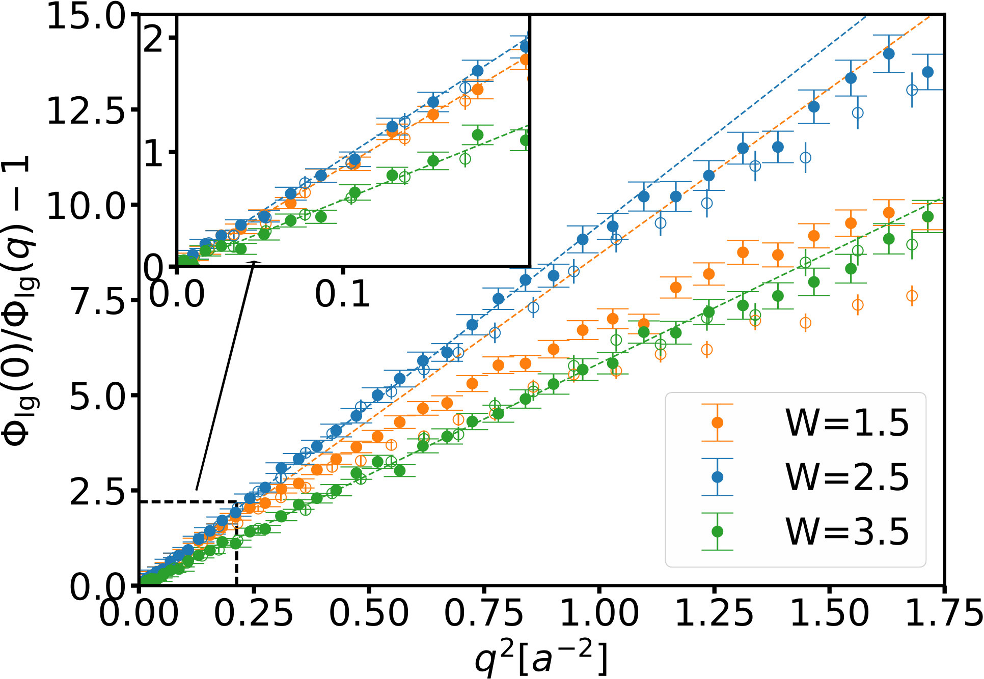 Figure 7
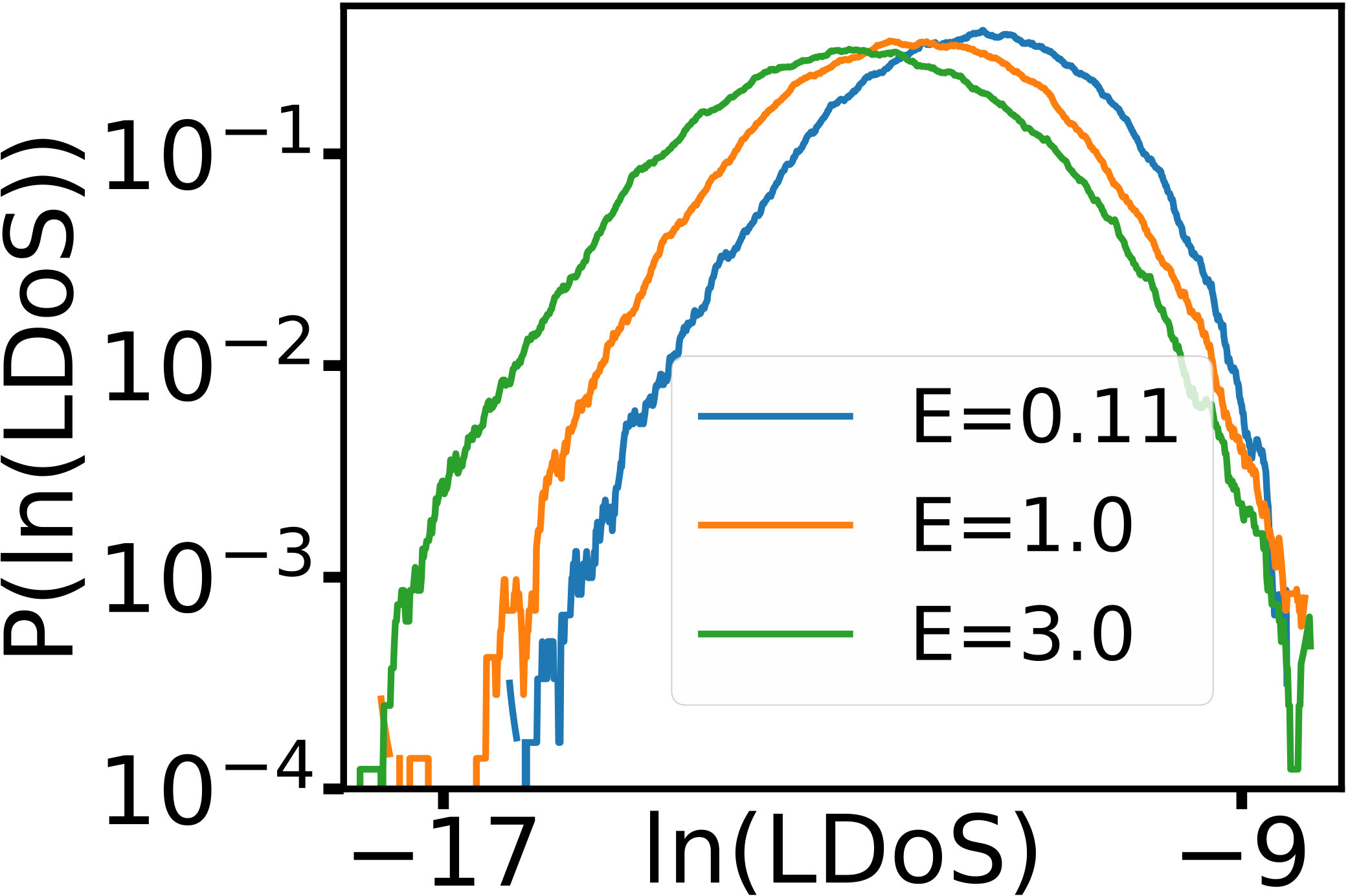 Figure 8
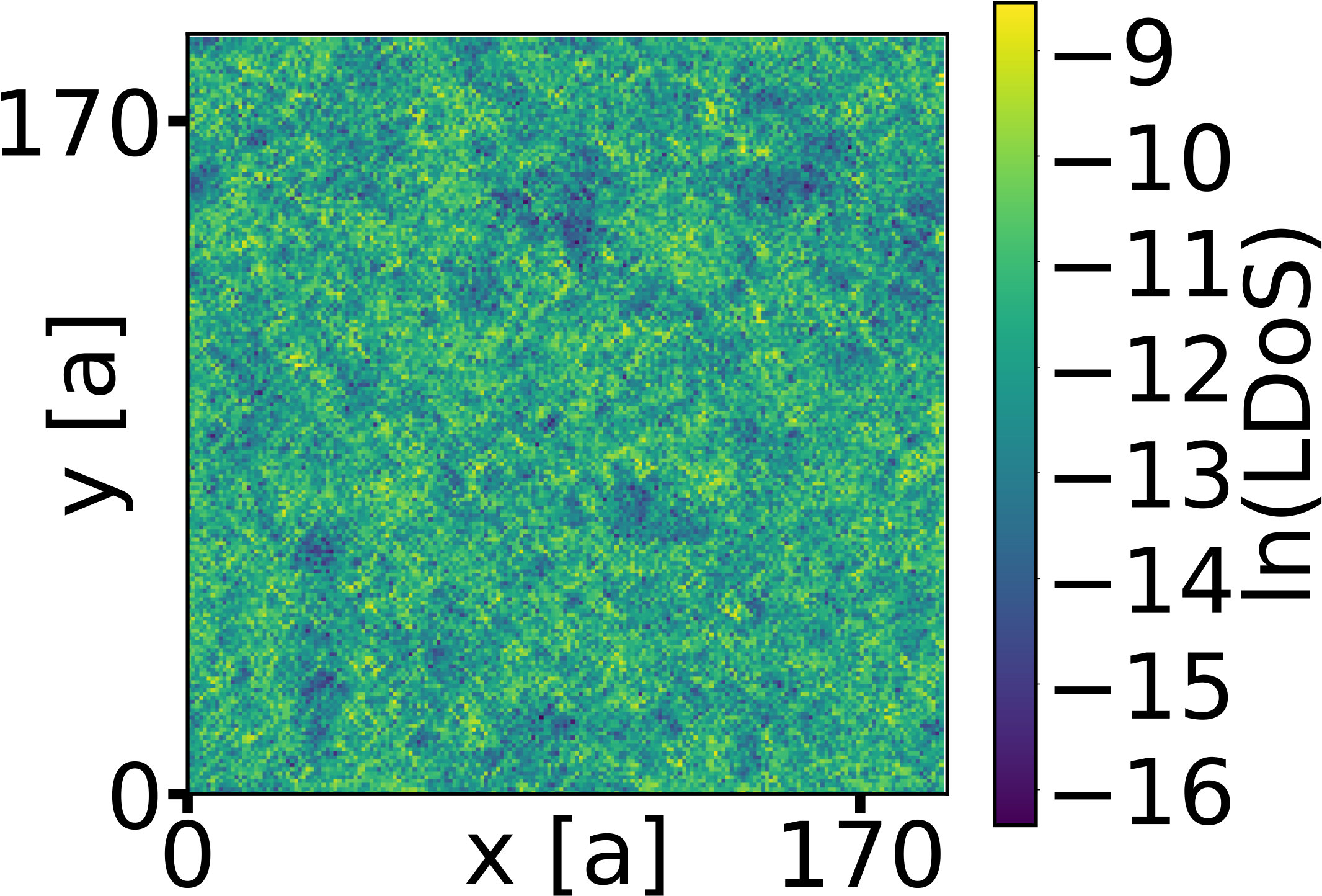 Figure 9
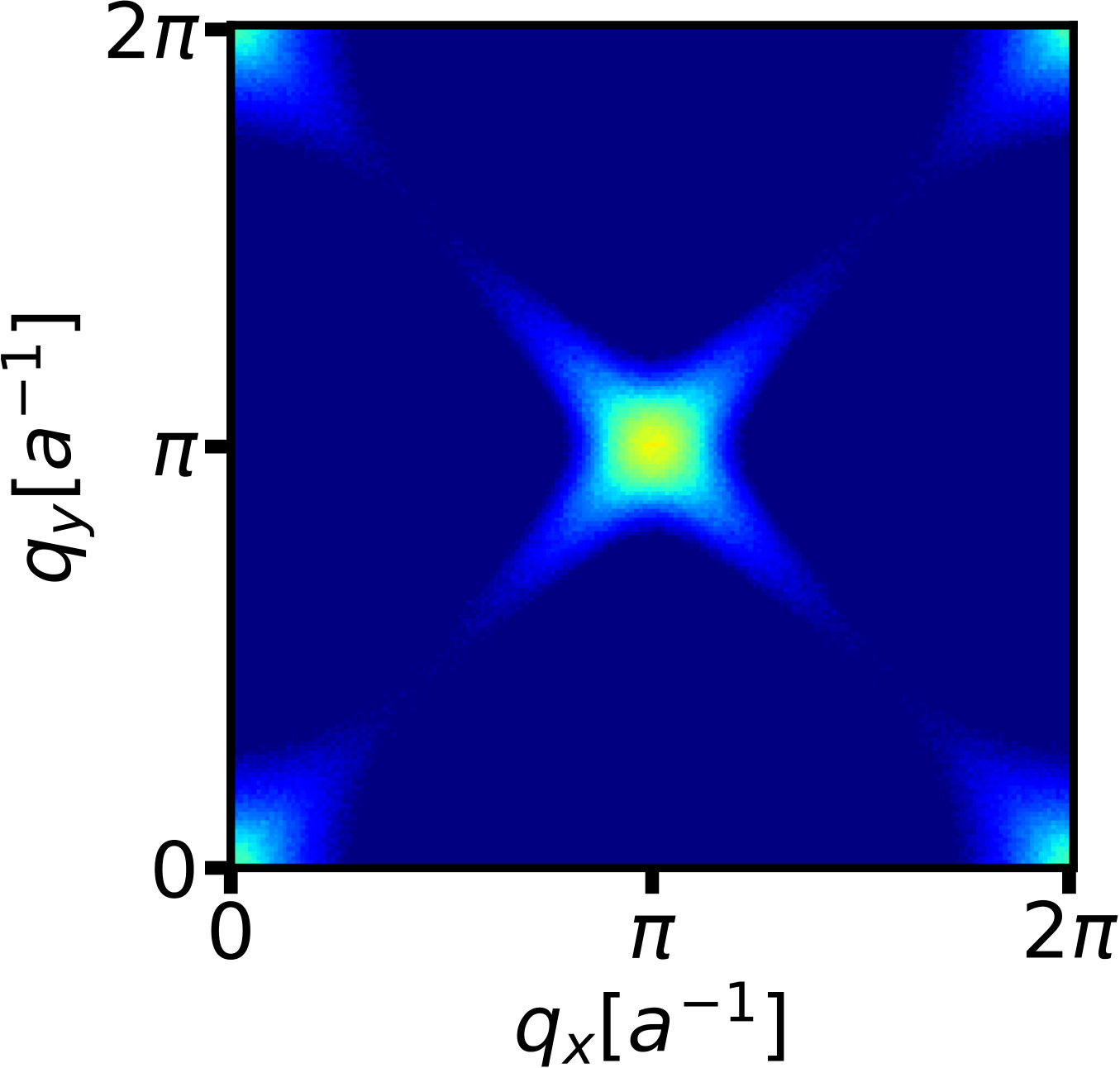 Figure 10
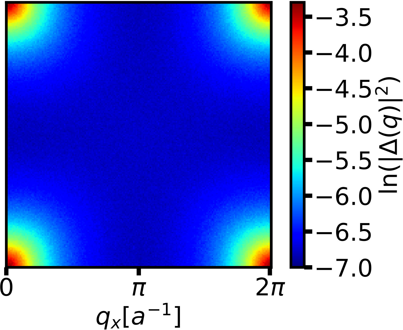 Figure 11
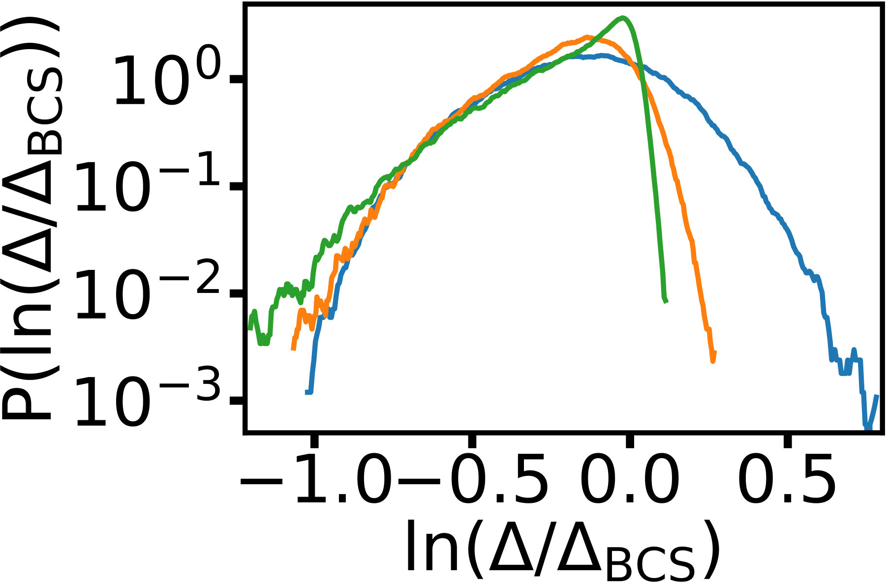 Figure 12
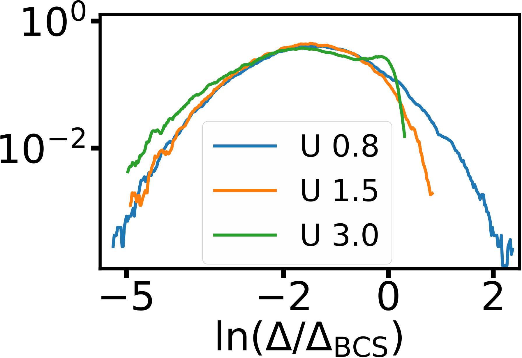 Figure 13
| dim | mean-field | observables | parameters | Ref. |
| IQHE | HF | Thouless numbers, IP | Yang et al. (1995) | |
| TDHF | ”Kubo conductivity” | Huckestein and Backhaus (1999) | ||
| 3D | HF | DoS, IP | Epperlein et al. (1997) | |
| 3D | HF | DoS, IP | Yang et al. (1995) | |
| 3D | HF | mf-dim | Amini et al. (2014) | |
| 3D | HF | DOS, mf-dim | Lee and Kim (2018) | |
| 3D | BdG | , LDoS | Covaci et al. (2010) | |
| s-wave | ||||
| 3D | DFT | mf-spectrum | Carnio et al. (2019) | |
| 3D | LDA | with | factor of | Harashima and Slevin (2012, 2014) |
| KS-states | two in | |||
| 2D | BdG | DoS, | Ghosal et al. (1998, 2001) | |
| s-wave | ||||
| 2D | BdG | DoS, | Potirniche et al. (2014) | |
| s-wave | LDoS | |||
| 2D | BdG | DoS, | Ghosal and Kee (2004); Chakraborty et al. (2017); Ganguly et al. (2017) | |
| s-, d-wave | ||||
| 2D | BdG | , | Seibold et al. (2012); Lemarié et al. (2013); Cea et al. (2014); Seibold et al. (2015) | |
| s-wave | ||||
| 2D | BdG | Dubi et al. (2007) | ||
| s-wave |
Peer Reviews
No public reviews on file for this paper yet. If you reviewed it on a platform where reviews are public (OpenReview, ICLR, NeurIPS, ICML), you can paste yours below so the community can read it here.
Videos
No videos yet. Explain this paper in a talk, walkthrough, or lecture? Add one.
Self-consistent-field ensembles of disordered Hamiltonians:
Efficient solver and application to superconducting films
Matthias Stosiek
Institute of Theoretical Physics, University of Regensburg, D-93040 Germany
Bruno Lang
Institute of Applied Informatics, University of Wuppertal, D-42119 Germany
Ferdinand Evers
Institute of Theoretical Physics, University of Regensburg, D-93040 Germany
Abstract
Our general interest is in self-consistent-field (scf) theories of disordered fermions. They generate physically relevant sub-ensembles (“scf-ensembles”) within a given Altland-Zirnbauer class. We are motivated to investigate such ensembles (i) by the possibility to discover new fixed points due to (long-range) interactions; (ii) by analytical scf-theories that rely on partial self-consistency approximations awaiting a numerical validation; (iii) by the overall importance of scf-theories for the understanding of complex interaction-mediated phenomena in terms of effective single-particle pictures.
In this paper we present an efficient, parallelized implementation solving scf-problems with spatially local fields by applying a kernel-polynomial approach. Our first application is the Boguliubov-deGennes (BdG) theory of the attractive- Hubbard model in the presence of on-site disorder; the sc-fields are the particle density and the gap function . For this case, we reach system sizes unprecedented in earlier work. They allow us to study phenomena emerging at scales substantially larger than the lattice constant, such as the interplay of multifractality and interactions, or the formation of superconducting islands. For example, we observe that the coherence length exhibits a non-monotonic behavior with increasing disorder strength already at moderate . With respect to methodology our results are important because we establish that partial self-consistency (”energy-only”) schemes as typically employed in analytical approaches tend to miss qualitative physics such as island formation.
Superconductor-Insulator Transition, Multifractality, Mean-field Theory, Hubbard Model, Kernel Polynomial Method
I Introduction.
The symmetry classification of disordered metals as it has been devised by Altland and Zirnbauer is nowadays considered to be complete.Zirnbauer (1996); Altland and Zirnbauer (1997); Heinzner et al. (2005) The classification is fundamental in the sense that all generic ensembles of random Hamiltonians have been covered. The classifying criterion is the presence or absence of one of the four elementary symmetries: time-reversal, spin-rotation, sublattice (chiral) and particle-hole (Boguliubov-deGennes-type).
Based on an (incomplete) analogy to the conventional Landau-Ginzburg-Wilson theories of classical phase transitions, there was a wide-spread misunderstanding with many researchers at the late 1980ies and early 1990ies that a classification based on symmetry (and topology) alone would (more or less) determine the phase-diagrams and the associated critical points as well. In other words, the symmetry-classification was largely identified with a classification of universality classes, i.e. of all non-equivalent quantum field theories (low-energy action-functionals) that describe a disordered electron system. Therefore, it came as a surprise for the larger part of the community when models of disordered fermions had been found that formally belong to the same symmetry class but nevertheless exhibit different phase diagrams.
It is perhaps fair to say that despite of the progress in the symmetry classification, we are still far from a systematic understanding of all universality classes and phase-diagrams that systems of disordered fermions could exhibit. One could rephrase by saying that the generic ensembles of random Hamiltonians covered in the ten-fold way possess physically relevant sub-ensembles that exhibit their own phase-diagrams and critical fixed-points. The power-law random-banded matrices (PRBM) constitute a well studied example.Mirlin et al. (1996) It offers a laboratory for criticality that can be addressed relatively easily with analytical and numerical techniques. Mirlin et al. (1996); Mirlin and Evers (2000)
I.1 General motivation for investigating scf-ensembles
The appearance of criticality in the PRBM-ensemble is a synthetic property; it is imposed by putting long-range (power-law) correlations into the hopping amplitudes of a tight-binding Hamiltonian. It therefore is interesting to explore properties of other ensembles that also exhibit long-range correlations in the Hamiltonian matrix elements, but of a kind that is self-generated and in this sense ”emergent”. Plausible candidates for such Hamiltonians are effective single-particle systems that appear in self-consistent-field (scf-) theories of interacting fermions. A prototypical example could be the Hartree-Hamiltonian of a disordered wire or film; it carries a long-range correlated on-site potential due to a weakly screened Coulomb-interaction.
Quite generally, we have in mind fermionic Hamiltonians
[TABLE]
the matrix is a functional of the density matrix and the pairing fields . The self-consistency condition inherent to generic mean-field theories requires that the fields and are expectation values of operators to be calculated employing - amongst other ingredients, such as density matrices or exchange-correlation kernels – also . Thus, scf-conditions are implied,
[TABLE]
that and obey.
A microscopic randomness will enter , e.g., via incorporating random on-site energies or hopping amplitudes. The set of random Hamiltonians introduced thereby follows the conventional symmetry classification. However, only the subset of all members of a given symmetry class that happens to comply with Eq. (2) forms the scf-ensemble.
We believe that scf-ensembles, their physical and mathematical properties constitute a fundamental research topic that may not yet have received the amount of attention it deserves. Our belief bases on two observations: (i) The elements of scf-ensembles certainly tend to exhibit non-trivial correlations in their matrix elements and . If correlations happen to be strong enough, e.g. sufficiently long ranged, then new phases with novel critical behavior can be expected to emerge. (ii) Mean-field theories are important because they provide a tractable reference point for a perturbative analysis of interaction effects. Thus, they are a generic encounter in all theories of disordered fermions that try to incorporate interactions. To reveal, in particular, the impact of quantum fluctuations a thorough understanding of the mean-field reference point would certainly seem helpful.
We give examples for occurrences of scf-ensembles:
Hartree theory (H)
The obvious example to define ensembles of self-consistent Hamiltonians would be the Hartree-theory. In this case and the field in Eqs. (1) and (2) should be identified with the particle density .
Hartree-Fock theory (HF)
; resembles the density matrix and the Fock-operator.
Density-functional theory (DFT)
In the orthodox flavor , represents the particle density and becomes the Kohn-Sham-Hamiltonian. Roughly speaking, DFT differs from HF due to the presence of correlations in .
Boguliubov-deGennes-Hamiltonian (BdG)
The basic Hamiltonian is given in Eqs. (1) and (2).
Our short list is far from exhaustive and further examples could be given. For instance, we recall that many spin-systems have faithful representations in terms of fermionic network-models that also could be dressed with self-consistency requirements, like self-consistent fluxes.
Remarks:
(i) The investigation of scf-ensembles is a very challenging endeavor. The difficulty is that each disorder configuration requires to find its own self-consistent fields and . The solution of the scf-cycle is very difficult to do with analytical techniques. But also numerically it is demanding already at moderate system sizes of a few thousand sites. Consequently, the number of studies including full self-consistency appears to be limited. In Tab. 1 we list contributions most relevant to us.
(ii) A more general perspective can be developed that operates with self-consistency constraints on the Green’s function rather than on the elements of the Hamiltonian. The generalization becomes non-trivial when the self-energy picks up an energy dependence. As a prototypical example we mention the GW-theory. It constitutes an electronic-structure method that builds upon the Hedin-equations approximating them by ignoring vertex corrections.Hedin (1965) In its full flavor the theory features a Green’s function that satisfies a self-consistent set of equations defined by a truncated diagrammatic expansion. Bechstedt (2015); van Setten et al. (2013)
(iii) A potential classification scheme of scf-ensembles will involve concepts very different from the one designed by Altland and Zirnbauer (AZ). To see this, we recall that AZ distinguish ten classes according to presence or absence of discrete symmetries. In contrast, the scf-requirement as formulated in (2) invokes parameter-bound kernels. Hence, a priori the number of scf-ensembles is not limited and an impression might arise according to which the scf-ensembles carry a degree of arbitrariness and therefore are less fundamental. To address this reservation against the basic concept, we recall that there is a very special set of scf-theories which is standing out; these scf-theories share with the parent field theory they derive from the basic symmetries and in this sense are conserving.Kadanoff and Baym (1962) Therefore, a classification of conserving scf-ensembles goes together with the basic program of condensed-matter theory, which is to identify and understand the fixed-point theories that are possible within a given AZ symmetry class.
I.2 Motivation for numerics and challenges
The numerical challenge that the scf-ensembles pose as compared to simulations of noninteracting fermions is that for each sample the scf-equation Eq.(2) has to be solved in an iterative fashion. Since the ensemble average requires solving hundreds of samples, typically, the computational cost for such studies is extensive. Presumably, this is the main reason why numerical studies of scf-ensembles have been performed infrequently in the past, despite of their obvious fundamental relevance.
Thus motivated, we here present an implementation of the scf-problem that allows to achieve relevant system sizes at an affordable numerical cost. The interplay of disorder induced quantum-interference and mean-field interactions can be studied on length scales that exceed the lattice constant by two orders of magnitude.
Reduction of scaling - KPM:
The computationally demanding step limiting the code-performance is the calculation of the scf-fields, , and , that need to be evaluated in every iteration cycle of the self-consistency process. In the case of Hartree-Fock-theory, for instance, this implies the reconstruction of the density-matrix from a given Fock-operator. In straight-forward implementations the Hamiltonian is diagonalized in each iteration cycle to feed eigenvalues and eigenvectors into the rhs of (2); the cost is operations, where is the dimension of the single-particle Hilbert space. iiiOnce the scf-field was found an update of has to be computed. This computation is efficiently dealt with by employing the fast Fourier-transformation (FFT) and therefore not critical. With FFT an operation that formally is can be downgraded to .
Consider the Hartree-approximation: the matrix diagonalization appears, because the trace
[TABLE]
contains the Fermi-Dirac function, , of a matrix valued argument that conventionally is evaluated in the basis of eigenstates of .
What many suggestions for -solvers, , of the self-consistency problem have in common is that they employ an alternative approach for trace-computation that avoids a diagonalization of and therefore can be more efficient, in principle, than . One of the well established options is the kernel-polynomial method (KPM). Weiße et al. (2006) The conceptual idea behind this approach is to expand into a rapidly converging series of Chebyshev polynomials, , that are obtained recursively:
[TABLE]
where denotes an appropriately scaled Hamiltonian and is a suitable basis in which is sparse. (: order of the Chebyshev expansion; : known expansion coefficients; : number of basis functions). As is seen from (4), the evaluation of the trace is of order . denotes the number of non-zero entries of per row. For a dense matrix we have , while for a very sparse matrix . For example, the BdG case, we have , with denoting the number of nearest neighbors on a cubic lattice in dimensions.
Signatures of implementation:
We have implemented a matrix-free KPM-solver of the self-consistency problem (1), (2) for the situation where the self-consistent fields are local in real space and , as is the case for the Hartree approximation and the Boguliubov theory of s-wave superconductors. It operates at zero and non-zero temperature and is optimized, for accelerated convergence for averages over the phase-space of disordered scf-ensembles.
The KPM-aspect of our implementation is similar to other variants described in earlier work. They have been proven useful in applications of the BdG-equation for nanostructures with one or very few impurities, but have not been applied to disordered samples. Implementation differences are in details: Covaci et al. (2010); Nagai et al. (2012, 2013) also use KPM to perform traces. In addition, Covaci et al. (2010) also have employed a matrix-free implementation. While these authors expand the Green’s function employing the Lorentz kernel, we expand the spectral function where the Jackson Kernel typically has better convergence properties Weiße et al. (2006).
I.3 Application to dirty superconductors
Motivated by experiments on the superconductor-insulator transition, e.g. Ref. Baturina et al. (2007) and Sacépé et al. (2008), the attractive Hubbard model with on-site disorder has been studied recently in several computationalDubi et al. (2007); Bouadim et al. (2011); Seibold et al. (2012); Lemarié et al. (2013); Cea et al. (2014); Potirniche et al. (2014); Seibold et al. (2015); Cea et al. (2015); Loh et al. (2016) and analytical works.M. V. Feigel’man et al. (2007, 2010); Feigel’man and Ioffe (2015)
Important insights have been gained within the framework of BdG-theory. The most striking findings include (i) the granularity of the pairing amplitude (”islands”) emergent on the scale of the coherence length even for short-range disorderGhosal et al. (2001); (ii) the parametric decoupling of the spectral gap from the mean pairing amplitude at large disorder: while the first remains relatively large the second decays to zero. Ghosal et al. (2001) (iii) A parameter regime was predicted where the typical size of pairing amplitude is increased as compared to the clean limit, so disorder has a pronounced tendency to enhance superconductivity. The mechanism was explored in 3D near the Anderson transitionM. V. Feigel’man et al. (2007, 2010) but also in 2D samples with short and long-range interactionsBurmistrov et al. (2012, 2013, 2015). Several predictions are broadly consistent with numerical results obtained on a honeycomb lattice Potirniche et al. (2014). (iv) At large interactions the coherence length was reported to exhibit a non-monotonous behavior with increasing disorder strength.Seibold et al. (2015)
Despite the progress the current situation is not fully satisfying: On the one hand side, computational studies of BdG-Hamiltonians have been limited to system sizes that do not allow to study the most interesting regime of length scales where the coherence length exceeds the lattice spacing: . While analytical approaches, on the other hand, operate in this regime, they rely on partial self-consistency in order to become tractable.
Motivated by this observation, we investigate as a first application of our technology the BdG-problem of disordered superconductors focussing on -wave pairing in thin films at . The full parameter plane of disorder, , and interaction, , is considered in which we study the distribution function and autocorrelations of the local gap function, , as our main observable. Our computational machinery allows us to cover the full parameter space from the extreme regimes, which have been addressed computationally before, to the analytically tractable weak coupling limit. In this effort we observe the formation of islands in large regions of the parameter space, for the first time on mesoscopic scales considerably exceeding the lattice constant. Regimes are included with parameters relatively close to the one where strong inhomogeneity has been observed experimentally.Sacépé et al. (2011).
Our observation might indicate that islands play a crucial role for the stability of the superconducting phase in actual experiments. Namely, islands imply localized Cooper pairs and therefore a diminishing of the phase-stiffness. In other words, islands go together with enhanced phase-fluctuations that destabilise long-range superconducting order. This connection between island-formation and stability has been emphasized before.Ghosal et al. (2001); Dubi et al. (2007)
Calculating the autocorrelation function of the spectral gap, we can extract a characteristic inverse length scale with the physical meaning of a correlation length. We study within the full phase diagram. Interestingly, concomitantly with island formation we find an enhanced BdG-coherence length. A similar observation if only at very large interaction strength, , has been made by Seibold et al. (2015). To what extent the enhancement of is an artefact of mean-field theory that is removed when adding phase fluctuations remains to be seen.
Finally, like earlier authorsGhosal et al. (2001) we also pay a special attention to the sensitivity of the behavior of computational observables to approximations made in the self-consistency procedure. We find that the island formation when observed in moderate parameter regions is a characteristic hallmark of full self-consistency; it escapes partial (“energy-only”) self-consistent schemes. We conclude that the renormalization of wavefunctions associated with full self-consistency will probably be an important ingredient of a qualitative theory of the superconductor-insulator transition.
II Model and Implementation
II.1 BdG-treatment of Hubbard model
We consider the attractive Hubbard model Hubbard (1963) on the square lattice in two-dimensions within the mean-field (BdG-type) approximation:
[TABLE]
with local occupation number , pairing amplitude , and random potential drawn from a box distribution. We employ periodic boundary conditions and work at ; the chemical potential is adjusted to fix the the filling factor to . iiiiiiThe filling factor is chosen in a way to be close to half-filling, which favors a high particle-hole overlap, while avoiding the ground state degeneracy of the superconducting state with a charge density wave state at half-filling.
This Hamiltonian is diagonalized by a Bogoliubov transformation
[TABLE]
The particle and hole wave functions and are determined solving the BdG equation
[TABLE]
where the physical sector corresponds to and
[TABLE]
the sum over is over the lattice sites neighboring . The scf-conditions for the density and the gap-function read
[TABLE]
We assume self-consistency to be attained, if the relative change per iteration cycle in is at each site smaller than . Typical values we take are . Note that the average change per iteration cycle is much smaller than , e.g., for a typical sample at moderate disorder we have
II.2 Matrix-free implementation of sparse-matrix vector product
To speed up a single self-consistency iteration we optimize the Chebyshev expansion. Its performance critical part constitutes of the recursive action of the Hamiltonian on a basis vector, Eq. (4). An implementation of the sparse-matrix vector product custom-tailored to our system is crucial for an optimal performance. The sparse-martrix vector multiplication is memory-bound, i.e. the performance is limited by the time it takes to fetch data from memory. For this reason we devised a self-written ”matrix-free” matrix vector product that outperforms standard state of the art sparse-matrix vector multiplication libraries.
The idea is the following: Conventional sparse matrix packages keep all non-zero elements, i.e. value and index, in memory. Matrix-free implementations become efficient if many of the non-zero elements have identical values storing only the different values that occur.
With matrix-free implementations the graph of the Hamiltonian has to be hard-coded in the matrix-vector product routine. For our Hamiltonian the amount of memory load operations of matrix data is reduced by a factor of 6 reflecting the number of non-zero elements per row of . In addition, the integer indices corresponding to the matrix graph do not have to be loaded. Altogether, this leads to a reduction of data to be loaded by a factor of 9. iiiiiiiiiThe datatype for values is double and for the indices is integer. Note, that the speed-up to be expected from the matrix-free implementation is less than a factor of 9. This is because not only the matrix but also the basis vectors have to be loaded from memory, so the reduction of memory load operations also depends on how many basis vectors are acted on in parallel. We mention that recently a library has been made available that automatizes the implementation of such a matrix-free matrix-vector product for a given Hamiltonian Pieper et al. (2017).
II.3 Improved convergence of scf-cycle
We improve the code performance by reducing the number of iterations needed until the convergence of the scf-cycle. The main idea applies, e.g., when scanning the parameter space at fixed for increasing disorder strength . At strength a converged solution is found for a given disorder realization. Thereafter, a sample at larger strength is generated by rescaling the disorder in the first sample by a factor of . Then, will be used to initialize the scf-cycle for the second sample.
II.4 Scaling and Design Considerations
As almost all runtime is spent on the recursive matrix vector products, the code lends itself very well to being split in an efficient low-level (i.e. C) kernel embedded in a high-level (i.e. python) code that implements the rest of the self-consistency cycle in a convenient way with negligible loss of performance. The kernel has been optimized for both threading and vectorization. In Fig. 1 we show benchmarks performed on a compute node
with two 14-core Haswell Xeon Processor E5-2697 v3; we monitor the time spent for performing a single sparse matrix-vector product. Fig. 1 (left) is illustrating the efficiency of our intra-node (OpenMP) parallelization. For the investigated system sizes the memory-bound runtime limit is not yet reached as is evidenced by the high speedup through parallelization. This makes it very advantageous to perform calculations in this size regime, where parallelization can still be utilized effectively. Fig. 1 (right) compares our matrix-free implementation with the standard MKL. As is seen from the data, our matrix-free implementation is advantageous already at system sizes as small as sites. Note, that at such small system sizes even full diagonalization routines can compete. As a technical remark we mention that, in principle, the matrix-free code should always be faster as compared to MKL implementations. The crossover size originates from our decision to use python as a platform, which leaves an interface to a C-based kernel. This interface is plagued with a small overhead that becomes negligible beyond the cross-over size.
An additional level of parallelism is obtained by running the expansion of different basis vectors independently on different nodes. The average over the disorder ensemble is performed via farming. This inter-node parallelization scales almost perfectly.
III Results: BdG-study of disordered superconductors
III.1 Mesoscopic fluctuations of LDoS and local gap function
As a first application of our technology, we investigate statistical properties of and of the local density of states (LDoS), , throughout the -plane. To give a first impression we display in Fig. 2 (left) the gap function averaged over a suitable ensemble of disordered samples, ; the overline indicates the ensemble average with disorder configurations, typically samples. The data has been obtained on a square lattice and should be compared with an analogous plot produced on the honeycomb lattice by Potirniche et al. (2014). The gap enhancement seen for the honeycomb lattice is not reproduced in Fig. 2. This is somewhat surprising, perhaps, because the phenomenon on the honeycomb lattice has been interpreted in terms of analytical results from quantum-field theoryBurmistrov et al. (2015), which also should apply to the square lattice.
Also displayed in Fig. 2 (right) is the density of states, , calculated for four samples in representative regions of the parameter plane. At weak disorder the spectral gap and the coherence peaks are readily identified. Notice that only in the limit of weak disorder the spectral gap and scale with each other. Ghosal et al. (2001)
To characterize the statistical properties of physical observables we focus in the following on autocorrelation and distribution functions. We will compare numerical findings with predictions from analytical theories and, in particular, study the sensitivity of qualitative results on modifications in the scf-conditions.
III.1.1 Distribution functions of LDoS and local gaps
LDoS.
We begin the statistical analysis with the spatial fluctuations of the LDoS, . Fig.3 (left) displays an example showing how the LDoS is spatially distributed over a typical sample with moderate disorder and interaction, . The logarithmically broad distribution, , is readily identified. The corresponding distribution function is displayed in Fig. 3 (right). It takes a log-normal form, already familiar for disordered films with size smaller than a localization length, see e.g. Eq. (4.101) in Ref. Mirlin (2000).
With increasing energy the distribution shifts to smaller values, which is merely reflecting the decrease of the DoS , also seen in Fig. 2 (right). In contrast, the width of is seen to grow. We assign this growths to the fact that the LDoS constitutes an average taken over a fixed-size energy window . The number of eigenfunctions in the averaging window is estimated as and therefore changes in energy if the DoS does. It is larger for energies near the coherence peak as compared to the bulk and for that reason the width of should be expected to be reduced.
The LDoS-distribution has been investigated analytically at temperatures above the critical temperature . Burmistrov et al. (2016) Our observations are broadly consistent with these results, since it is reported that the distribution develops a pronounced non-Gaussian character upon decreasing the temperature. For a more quantitative comparison, simulations at finite temperatures are required that are under way. Stosiek et al.
Local order parameter.
The logarithmically broad distribution of the LDoS is concomitant with a similarly broad distribution of the local gap function , Fig. 4.
The evolution of the latter function with interaction strength is very interesting. As long as disorder, , and interaction, , are weak the distribution of the local order parameter is close to Gaussian and in this sense roughly following the statistics of the LDoS, see Fig. 4 (left). The typical value is seen to be very close to the pairing amplitude of the clean system, . However, with growing the weight of untypically large values of is seen to be suppressed rapidly, while the weight of untypically small values is rather resilient.
For increasing disorder and weak more and more sites develop a pairing well below the clean limit, , consistent with observations made in Ref. Ghosal et al. (2001). Eventually, the shoulder is seen to dominate, Fig. 4 (right) and the distribution becomes bimodal. It features a peak near and a logarithmically distributed background. The bimodal shape of is apparent also from Ref. Lemarié et al. (2013) where it is seen at very large interaction, .
III.1.2 Autocorrelations of gap function and coherence length
We consider the disorder averaged spatial autocorrelator of the pairing function in Fourier space.
At weaker disorder the correlation function displays a peak at , Fig. 5. It originates from us choosing the filling fraction which is close to the commensurate value unity and thus should be seen as a signature of the square lattice; it disappears at stronger disorder, e.g., at . The same signature manifests in Fig. 6 where we show along two directions in -space, and : As already obvious from Fig. 5, at wavenumbers of order of the inverse lattice spacing, , and low the correlator exhibits pronounced deviations from isotropy reflected by the collapse of open and closed symbols.
Notwithstanding anisotropy at , in the limit of small wavenumbers the correlator is isotropic and with good accuracy we have
[TABLE]
where , given for different in Fig. 7. behaves nearly quadratically over the whole momentum range where exhibits isotropic behavior. Both the increase of (as approximated by ) with disorder and the characteristic length have been displayed in Fig. 7.
To attain we have used a linear fit of in the isotropic regime. As with the range of this regime also the number of data points increases considerably with , the uncertainty, i.e. the size of the error bars, of is seen to decrease with rising in Fig 7 (left). exhibits a local non-monotonicity on its way from the clean to the dirty limit; the non-monotonic decay is readily seen also from the original data Fig. 6. This peculiar behavior should be interpreted in connection with the formation of superconducting islands. It occurs in the same parameter range and may relate to a percolation transition. Our data shows that the non-monotonous shape, which was found in Ref. Seibold et al. (2015) albeit at unrealistically strong interactions , carries over all the way into the physically more relevant regime of intermediate parameter values.
IV Impact of self-consistency
We return to a central theme of our interest, which is the impact of self-consistency on the calculation of physical observables.
IV.1 Partial (energy-only) self-consistency scheme
The full BdG-problem is specified by the set of equations (14) - (18). It is highly complicated, e.g., because the scf-conditions (17) and (18) are non-linear. As is frequently done in such situations, the full scf-problem is replaced by a simplified variant exhibiting partial self-consistency.
Various possibilities for such simplifications are conceivable. The scheme we here describe is inspired by analytical calculations performed by Feigelman et al. M. V. Feigel’man et al. (2007, 2010). The overall procedure can be considered a generalization of BCS theory that allows for an inhomogeneous order parameter. To bring the self-consistency requirement into the familiar BCS form, additional approximations besides the mean-field decoupling are necessary.
We here derive equations for partial self-consistency starting from the mean-field Hamiltonian Eq. (5). We express the field operators employing as a basis the eigenstates of the non-interacting part of , i.e. :
[TABLE]
The corresponding eigenvalues of are denoted and will be measured with respect to the Fermi-energy . Expressing in we obtain
[TABLE]
where an abbreviation
[TABLE]
has been introduced.
The main approximate step in partial self-consistency is to neglect all terms with more than two indices
[TABLE]
together with the Hartree term. The simplified mean-field Hamiltonian then reads
[TABLE]
with an s-wave pairing strength
[TABLE]
The Hamiltonian (24) is structurally equivalent to the BCS Hamiltonian in the sense that the kinetic term and are diagonal in the same (real-space) basis; Cooper pairs form within a Kramer’s doublet. The corresponding BCS gap-equation reads
[TABLE]
Converting back to real-space we have
[TABLE]
The advantage of the partial (“energy-only”) scf-scheme is that the pairing-amplitude can be calculated solely from the eigenstates and eigenvalues of the non-interacting reference Hamiltonian . This comes at the expense of ignoring changes in the wavefunctions related to pairing and the inhomogeneous Hartree shift.
IV.2 Effects of self-consistency schemes on the local-gap distribution
We compare the results of full and energy-only self-consistency schemes for the local pairing amplitude for the Anderson Problem in 2D and 3D.
2D
Fig. 8 shows a spatial distribution of as obtained for typical sample at intermediate interaction and three disorder values. The calculation with full self-consistency, Fig. 8 (left) column exhibits a clear tendency towards the formation of superconducting islands. In contrast, with energy-only self-consistency, right column, a rather homogeneous speckle pattern is found missing any indications of island formation. Hence, already by inspecting individual samples we expect that distribution functions of physical observables will depend in a qualitative way on the applied scf-scheme in broad parameter regions.
In order to highlight the effect of screening, we have displayed in Fig. 8 also the results of an intermediate scf-scheme. It operates in an energy-only mode, but adopts for the disorder the effective single particle potential (”screened” potential) as it is obtained as a result from the full scf-calculation. As is seen from Fig. 8, center column first indications of islands emerge, but the contrast is still largely underestimated. This result underlines the importance of full consistency in the scf-procedure.
3D
In analogy to the 2D case, we compare the results of full and energy-only self-consistency schemes for the local pairing amplitude in 3D.
In the non-interacting 3D Anderson problem there is a phase transition at a critical disorder strength , where all states become localized. For a disorder strength below there exists an energy , the mobility edge, which separates a fully localized band from a band of extended states. We note that as the Anderson Hamiltonian is symmetric around this is also true for the mobility edge. We refer to B. Bulka (1987) for the phase diagram.
Our interest is in the importance of self-consistency in the presence of attractive on-site interactions close to the mobility edge in the insulating band. For comparibility with authors that have considered an energy-only approach in this context beforeM. V. Feigel’man et al. (2010), we choose a Gaussian disorder distribution
[TABLE]
of the random onsite energies in Eq. 15.
Fig. 12 shows the spatial distribution of of a typical sample as obtained for moderate interaction and disorder strength and chemical potential in the localized band. The chosen filling factor corresponds to a chemical potential of in the fully self-consistent case. The mobility edge without interactions is located at for the disorder strength that is considered hereB. Bulka (1987). As in the 2D case, the field obtained within the fully self-consistent calculation shows a pronounced formation of islands, Fig. 12 (left). The energy-only scheme in analogy to our 2D results exhibits a rather homogeneous spatial distribution, Fig. 12 (right). The results of the energy-only scheme with ”screened” potential shown in Fig. 12 (center) again show first indications of island development with dramatically underestimated contrast. This highlights the importance of full self-consistency also in 3D.
To what extent the conclusions of earlier theoretical works that consider this scenario M. V. Feigel’man et al. (2007, 2010) are affected remains to be seen.
IV.3 Effects of self-consistency on gap autocorrelator
Fig. 10 shows data analogue to Fig. 6, now with energy-only self-consistencies. As is obvious already from individual sample, Fig. 8, the contrast parametrized by is much smaller as compared to the case of full self-consistency given in Fig. 5. As one would expect from Fig. 8, the contrast with screened potential, Fig. 8 (right) exceeds the bare scheme, Fig. 8 (left) considerably.
The most striking and perhaps unexpected feature, however, is a qualitative difference. In the full scf-calculation, follows Eq. (19) and exhibits a well defined parabolic shape in the vicinity of small wavenumbers. This feature is not reproduced within energy-only schemes. The bare scheme does not exhibit an appreciable curvature up to , so . In contrast, within the screened scheme does not show clear saturation at small wavenumbers within the range of -values accessible. We thus interpret these results as a strong indications that wavefunction renormalization as it occurs within the full scf-scheme is crucial for understanding those aspects of qualitative physics that hinge on long-range spatial correlations.
V Conclusions
We have implemented an efficient solver of self-consistent field (scf-) Hamiltonians that is based on the kernel-polynomial method. An application to disordered -wave superconducting films has been presented that employs the Bogulubov-deGennes approximation. The statistical properties of the local density of states and of the local gap function have been studied. In this context our computational machinery proves useful since system sizes can be accessed significantly exceeding the ones that have been achieved in the earlier work. We thus can study the crossover in disorder strength and interaction strength from the strongly coupled into the perturbative regime, where analytical methods apply and can provide conceptual insights.
Along this way three key observations have been made. (i) Superconducting islands form in large regions of the phase space and thus appear to be a typical encounter already at intermediate interaction and disorder strength. (ii) Presumably related to island formation, the (mean-field) correlation length exhibits a non-monotonous variation when sweeping from very weak to strong disorder. (iii) Island formation is a hallmark of wavefunction-renormalization in the sense that islands do not form with partial (”energy-only”) self-consistency. To investigate into possible consequences of this observation for analytical treatments of the superconductor-insulator transition we leave as a topic for future research.
As a concluding remark we note that the BdG-Anderson problem and the associated ensemble of self-consistent random Hamiltonians is a particular representative of a very large class of random matrices that satisfy a self-consistency constraint (”scf-ensembles”). Presumably, because of the considerable challenges that such ensembles imply for analytical and computational treatments very little is known about them. We take the observations that have been reported for the BdG-ensembles, in this work as well as by the earlier authors, as a strong indication that much is there to be discovered.
Appendix
Self-consistency cutoff discussion
In Fig. 11 the dependence of on at fixed is shown. The data demonstrates good convergence behavior of in terms of the cutoff-parameter ; in particular, the -dependency of is seen to be small as compared to the variation with . Figure 12 re-plots the data shown in Fig. 11, so the evolution of with is more clearly illustrated. In particular, it is seen that the non-monotonic behavior is very well converged in the cutoff . The stronger change of with seen at low disorder strengths, e.g. at , is related to the fact that the distribution of local values, is narrow at small . In this case, the convergence requirement allowing for a maximal percentage of change from cycle to cycle has implications for a substantial fraction of all sites; with broad distributions, convergence of most sites will be much better than .
Acknowledgement
We are grateful to Soumya Bera, Igor Burmistrov, Christoph Strunk and Thomas Vojta for numerous inspiring discussions; we also express our gratitude to Ivan Kondov for sharing mathematical and computational expertise. Support from the DFG under EV30/11-1 and EV30/12-1 is acknowledged. The authors gratefully acknowledge the Gauss Centre for Supercomputing e.V. (www.gauss-centre.eu) for funding this project by providing computing time on the GCS Supercomputer SuperMUC at Leibniz Supercomputing Centre (www.lrz.de). This work was performed on the supercomputer ForHLR funded by the Ministry of Science, Research and the Arts Baden-Württemberg and by the Federal Ministry of Education and Research.
The reference list from the paper itself. Each links out to its DOI / PubMed record.
- 1Zirnbauer (1996) M. R. Zirnbauer, J. Math. Phys. 37 , 4986 (1996).
- 2Altland and Zirnbauer (1997) A. Altland and M. R. Zirnbauer, Phys. Rev. B 55 , 1142 (1997).
- 3Heinzner et al. (2005) P. Heinzner, A. Huckleberry, and M. R. Zirnbauer, Commun. Math. Phys. 257 , 725 (2005).
- 4Mirlin et al. (1996) A. D. Mirlin, Y. V. Fyodorov, F.-M. Dittes, J. Quezada, and T. H. Seligman, Phys. Rev. E 54 , 3221 (1996).
- 5Mirlin and Evers (2000) A. D. Mirlin and F. Evers, Phys. Rev. B 62 , 7920 (2000).
- 6Hedin (1965) L. Hedin, Phys. Rev. 139 , A 796 (1965).
- 7Bechstedt (2015) F. Bechstedt, Many-Body Approach to Electronic Excitations (Berlin: Springer, 2015).
- 8van Setten et al. (2013) M. J. van Setten, F. Weigend, and F. Evers, J. Chem. Theory Comput. 9 , 232 (2013).