Wall Crossing Structures and Application to SU(3) Seiberg-Witten Integrable system
Qiang Wang (Kansas State University)

TL;DR
This paper applies wall crossing structures to SU(3) Seiberg-Witten systems, providing an algorithm to compute BPS invariants and discovering new BPS states with higher invariants.
Contribution
It introduces a novel algorithm using wall crossing formalism for calculating BPS invariants in SU(3) Seiberg-Witten systems, including new BPS states.
Findings
Algorithm for computing Donaldson-Thomas invariants
Identification of new BPS states with invariants equal to 2
Extension of known BPS spectrum in pure SU(3) case
Abstract
We apply the wall crossing structure formalism of Kontsevich and Soibelman to Seiberg-Witten integrable systems associated to pure . This gives an algorithm for computing the Donaldson-Thomas invariants, which correspond to BPS degeneracy of the corresponding BPS states in physics. The main ingredients of this algorithm are the use of split attractor flows and Kontsevich Soibelman wall crossing formulas. Besides the known BPS spectrum in pure case, we obtain new family of BPS states with BPS-invariants equal to 2.
Click any figure to enlarge with its caption.
 Figure 1
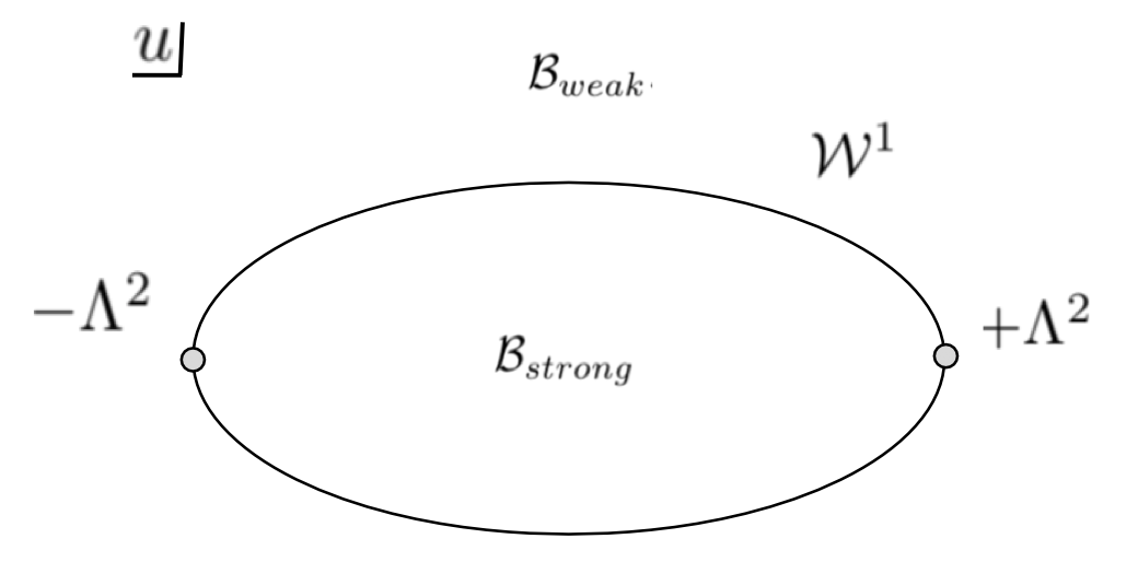 Figure 2
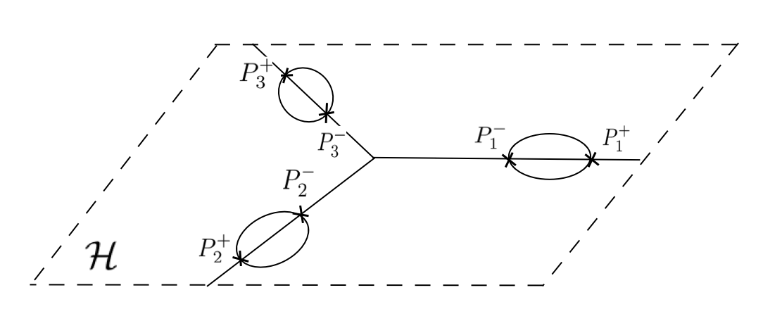 Figure 3
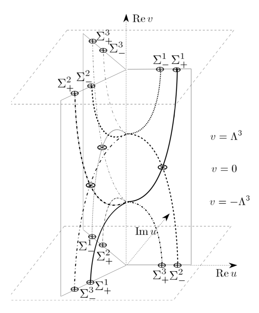 Figure 4
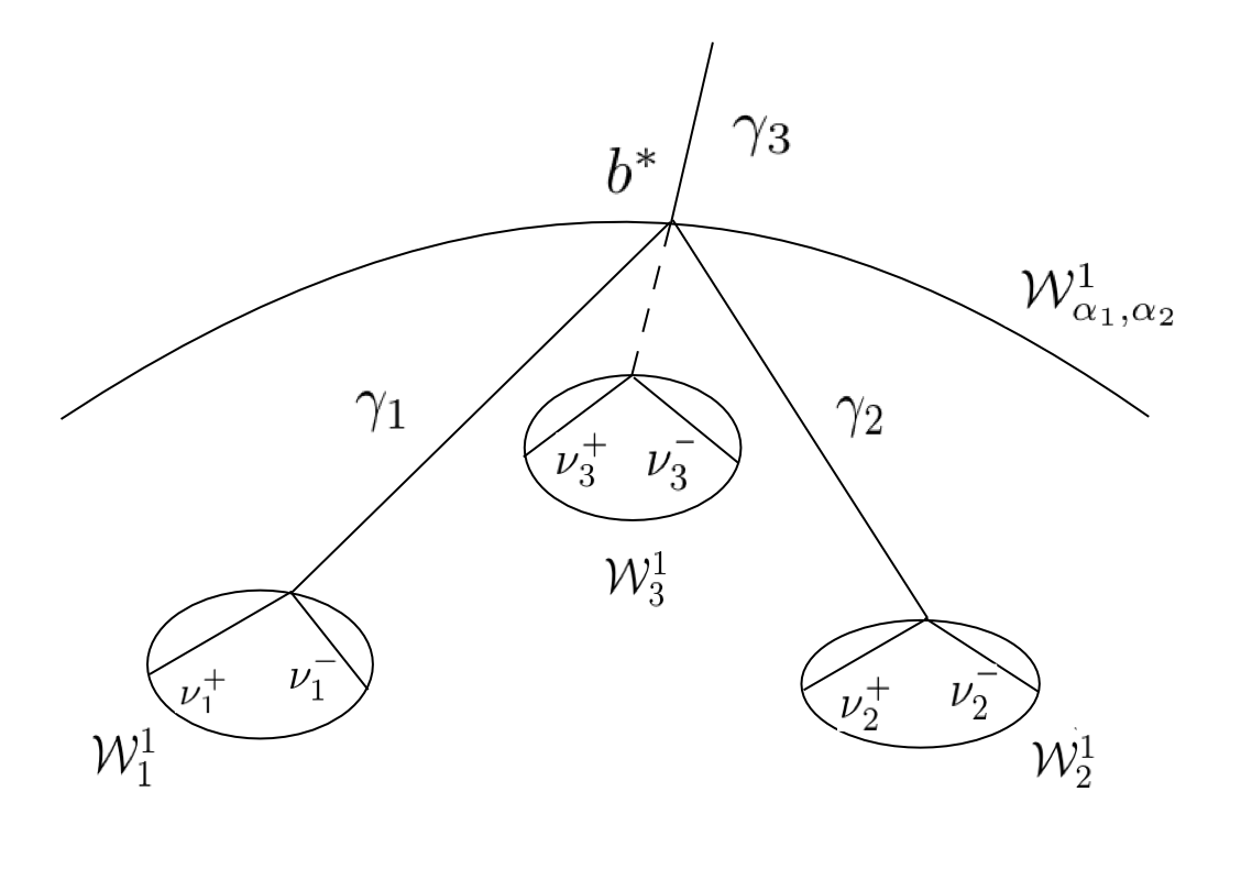 Figure 5
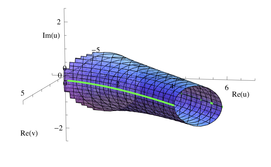 Figure 6
Peer Reviews
No public reviews on file for this paper yet. If you reviewed it on a platform where reviews are public (OpenReview, ICLR, NeurIPS, ICML), you can paste yours below so the community can read it here.
Videos
No videos yet. Explain this paper in a talk, walkthrough, or lecture? Add one.
Wall Crossing Structures and Application to SU(3) Seiberg-Witten Integrable system
Qiang Wang [email protected] Department of Mathematics, Kansas State University, Manhattan, KS, 66502
Abstract
We apply the wall crossing structure formalism of Kontsevich and Soibelman to Seiberg-Witten integrable systems associated to pure . This gives an algorithm for computing the Donaldson-Thomas invariants, which correspond to BPS degeneracy of the corresponding BPS states in physics. The main ingredients of this algorithm are the use of split attractor flows and Kontsevich Soibelman wall crossing formulas. Besides the known BPS spectrum in pure case, we obtain new family of BPS states with BPS-invariants equal to 2.
Contents
1 Introduction
The wall crossing structure ("WCS" for short) is a formalism proposed and studied by M.Kontsevich and Y.Soibelman in [1] that enables us to encode the Donaldson-Thomas (DT) invariants (BPS degeneracies in physics) and to control their "jumps" when certain walls (walls of marginal stability in physics) on the moduli space are being crossed. The celebrated Kontsevich-Soibelman wall crossing formula (”KSWCF" for short) [2] is an essential ingredient of WCS.
WCS formalism is well adapted to the data coming from the complex integrable system. The famous Seiberg-Witten integrable system (“SW integrable system" for short) ([3]) is an example. By considering certain gradient flows on the base of the integrable system called the split attractor flows(c.f.[4][5]), WCS can produce an algorithm for computing the corresponding DT-invariants inductively.
This paper is about applying the WCS to the SW integrable systems associated to the pure and supersymmetric gauge theories. We will see that the results via the WCS formalism match perfectly well with those obtained via physics approaches. ([6][7]).
The paper is organized as follows:
Section 2 gives a review of the formalism of wall crossing structures, which is based on the original paper of Kontsevich and Soibelman [1]. The review is tailored toward the application in section 4, thus some aspects of this formalism (for example, its connection to variation of Hodge structures) are missing in this biased review. We end the review in subsection 2.5 by analyzing in detail two examples of WCS, namely, the stability data and the parametrized family of stability data. The latter appears naturally in the framework of the complex integrable systems.
In section 3 we review the notion of complex integrable systems and its connection to the WCS formalism. We focus on the geometry of the base , which can be endowed with the structure of special Kähler geometry, as well as -affine structure. Then we can consider split attractor flows that are certain gradient flow lines on .
Finally in section 4, we apply the WCS to SW integrable systems for and . The main ingredients of the WCS for are the results of physics (see for example [8][9][10]). We just reformulate in terms of WCS.
The results of subsection 4.3, in which we constructed WCS for pure case, are new. The construction roughly goes as follows:
We know from [11][12][13] the vanishing cycles associated to the discriminant locus, which help producing the so-called initial condition of the WCS. The WCS is then studied by cutting the real four dimensional base with two complementary hyperplanes, so that the situation is reduced to the real two dimensional case. On the resulting plane after cutting, the discriminant locus was cut into six singular points that fall into three pairs, each of which determines a situation similar to the case considered in section 4.2. This corresponds to three embeddings of the Lie algebra . Thus, by applying the WCS formalism to this situation, we get three families of BPS states with non-trivial DT-invariants (or BPS invariants) (see proposition 4.9).
We apply again the WCS formalism to another wall (its existence is discussed for example in [7][14]) in order to derive the results about the interaction of the above three families. This gives us new BPS states with DT invariants equal to 2 (see proposition 4.11).
In [15], it is exhibited by using the method of spectral networks that even in this relatively simple case, the so called wild spectrum exists. The wild spectrum is characterized by the exponential growth of the DT-invariants. It would be very interesting to be able to produce the wild spectrum by using the WCS formalism considered in this paper. We leave the investigation along this direction for later works.
2 Wall Crossing Structures
Fix a lattice of finite rank, which is endowed with the pairing . We call the charge lattice. The central charge is an abelian groups homomorphism . Let be the -graded Lie algebra over ( is generated over by ), with Lie bracket:
[TABLE]
The support of is given by . We make the assumption that it is finite and contained in an open half-space in . In this case, is nilpotent. We denote by the corresponding nilpotent Lie group.
2.1 Nilpotent case
The wall associated to is the hyperplane . Denote by the finite collection of these hyperplanes. We borrow the following definition from [1]:
Definition 2.1**.**
A (global) wall crossing structure (WCS for short) for is an assignment such that for any which is locally constant in , and satisfies the following* cocycle condition***
[TABLE]
and such that in the case when the straight interval connecting and intersects only one wall , then we have that
[TABLE]
Denote the space of all WCS on by . Some easy consequences can be drawn from the above definition.
Lemma 2.1**.**
If the straight interval does not intersect any walls in , then . And for any , we have . More generally, for , we have
[TABLE]
Thus with any codimension one stratum , which is an open domain in for some , one can associate a “jump" . Here points and are separated by the wall and the straight segment intersects at a point belonging to . A WCS is uniquely determined by the collection of all jumps that satisfies the cocycle condition for each stratum of codimension 2.
2.2 Pronilpotent case
Let be strict sector (i.e., less than ) in , consider the pronilpotent Lie algebra . There exists such that its restriction to gives a proper map to . Then for , consider the quotient , where is the ideal consisting of elements with for . We get . Then for each , the WCS is defined on , and the WCS on corresponds to the one for the projective limit of . This can be done by using the sheaf theoretic description of WCS in subsection 2.4. Thus, for each , we have a formula similar to (4), and by taking the limit , we obtain:
Lemma 2.2**.**
For any , we have the following wall crossing formula:
[TABLE]
The (numerical) Donaldson-Thomas invariants proposed in [2] gives us a map (conjectured to be integer-valued). Using KS-transform: , for the ray , we attach the element:
[TABLE]
For strict sector and fixed , we have the truncation: (Lie group of ), and thus the finite product , where the right arrow indicates that the product is taken over all rays in clockwise order. Let , we get: . Clearly, . We identify the jump associated to with .
2.3 WCS on a topological space
A WCS on assigns for any pair a group element . We want to assign group element to a single point . It was shown in [1] (section 2.1.2) that there exists a sheaf of wall crossing structures over , denoted by , with the stalk over being [math] if , and a nontrivial element such that if belongs to some wall. for with general is defined as .
Let be a locally connected Hausdorff topological space. Given a locally continuous map , let be the pull back sheaf on , i.e., .
Definition 2.2**.**
(WCS on ): A (global) wall crossing structure on is a global section of the sheaf .
Given a section over open subset , (support of ) is the minimal closed subset of , conic in the direction of , that contains pairs such that and
Definition 2.3**.**
(walls of second kind in ) For every , the wall of second kind associated to it is defined as the pull back of through the map , that is:
[TABLE]
2.4 Wall Crossing Formulas
The WCS on is used to encode DT invariants that depends on . These invariants "jump" when certain walls on are crossed. These walls are called the wall of the first kind (walls of marginal stability in physics literature).
Definition 2.4**.**
For , the two -linear independent elements, we introduce the following set
[TABLE]
Then the so-called walls of the first kind associated to a charge are defined as .
The "jump" of DT invariants is controlled by the wall crossing formula of Kontsevich and Soibelman ([2]): Given an strict sector , does not depend on as long as there is no element such that crosses the boundary , i.e., it is locally constant as a function in near . Thus, when approaching to on the side of where proceeds in the clockwise order, would coalesce, and change the order after crossing the wall. But stays constant by the above discussion. By taking on both sides, the jump of can then be determined.
Consider the sub-lattice generated by the positive cone . Write simply as , the KSWCF then states that , which by using KS-transformation, it reads as
[TABLE]
Notice that the product on LHS (RHS) is taken over all coprime in the increasing (decreasing) order of .
Examples: The form of KSWCF depends on . gives the pentagon identity
[TABLE]
gives the following which is relevant to the representation of the Kronecker quiver :
[TABLE]
Finally, we point out that the formula (8) is equivalent to the WCF (5). Indeed, consider a loop around that intersects countably many walls of second kind . Then (8) can be informally interpreted as the triviality of the monodromy of along the small loop, i.e.,.
2.5 Examples of WCS
A stability data on (see [2]) is a pair consisting of a central charge and a collection of elements that satisfies the support property (we omit it here). Denote by the space of all stability data on . Since , where , is the same as the set which consists of pairs , where a collection of elements , with .
Example a): Take and consider , .
Proposition 2.3**.**
The WCS on induced by above is the same as a stability data.
Proof.
Given , recall that . Thus, if , i.e., , we can associate to a “jump" such that , where is the group element associated to . Then, the components of belonging to is deemed as . Conversely, given , it was shown in [1] (see section 2.1.2) that there exists element that determines uniquely a section of , which after pulling back through , gives arise to a section of . ∎
In order to recover , we consider the WCS on the space via the map
[TABLE]
Proposition 2.4**.**
A section of the sheaf on the space is same as a family of stability data on .
Proof.
For fixed , by restricting to , we get a stability data by above proposition. Moving locally, we get a germ of universal family of stability data with central charges near . ∎
Example b): Continuous family of stability data recovered
In application, we usually use a complex manifold to parametrize , which can be realized as the WCS on through the map
[TABLE]
Proposition 2.5**.**
A section of the sheaf on is same as a WCS on .
Proof.
Fix , we get a stability data on . As varies locally near , also varies locally around (as depends holomorphically on ). Thus by proposition 2.4, we get a germ of universal family of stability data near . But this is the same as a germ of universal family of WCS near . ∎
Given a WCS on , we get a locally constant map , where is the -component of the corresponding section of . Then is non-trivial only if there exists such that . Let , we see that restricts to .
Remark 2.1**.**
Since the map depends only on the -component of , so we will just call a WCS on as a WCS on , with the role of the circle being understood implicitly.
Recall from the definition 2.3, given , the wall of second kind associated to it is given by
[TABLE]
which is seen to be a hypersurface in . And the pull back of the wall of second kind in through the map . We can project this wall down to a hypersurface in , also denoted by , i.e.,
[TABLE]
3 Complex integrable systems and WCS
In this section, we review the notion of complex integrable systems following the treatment in [1] with emphasis on the connection to WCS. We will see that a WCS can be induced from the data of the complex integrable system. This produces an algorithm for computing DT-invariants by employing certain trees on its base given in terms of the split attractor flows.
3.1 Complex integrable system and its geometry
A complex integrable system (see section 4 of [1]) is a holomorphic surjective map with smooth fibers being holomorphic Lagrangian submanifolds, where is a holomorphic symplectic manifold of complex dimension , and the base is a complex manifold of dimension . Denote by the dense open subset over which the fibers being smooth, and by the discriminant locus. We make the assumption that the smooth fibres are compact, so they are actually holomorphic Lagrangian tori. It is well-known that:
Proposition 3.1**.**
The base of the complex integrable system is a -affine manifold.
Definition 3.1**.**
We have a local system of lattices over , with its “stalk" at being the first homology group . will be called the local system of charge lattices.
The one forms are closed, So locally holomorphic functions s.t. , which define an holomorphic map for an open neighborhood of .
Definition 3.2**.**
([1]) The collection of one forms gives rise to an element . If is zero, there exists a section , called central charge such that for .
If the fibers of are endowed with a covariantly constant integer polarization. We call such system the polarized complex integrable system. A polarization gives rise to . Denote by the corresponding matrix and by its inverse. We have that (section 4.1.1 of [1]):
Proposition 3.2**.**
a)
[TABLE]
In terms of the central charge , the condition a) and b) above can be rewritten as
[TABLE]
Choose symplectic basis for near . Then , where , are locally holomorphic on , called the special coordinates (see [16] for its definition). Then condition specialize into , from which we deduce that for some holomorphic function , called the prepotential. And we have: .
Condition becomes , thus we have the following Kähler metric on :
[TABLE]
where the matrix is given by .
Remark 3.1**.**
Define and , then are -affine coordinates on (see proposition 3.1). We can also use as -affine coordinates (dual affine structure). They differ by a -rotation of the central charge . More generally, we can consider the rotated -affine coordinates: or .
Near , the fibration degenerates. Some cycles, which we call the vanishing cycles shrink to zero. We give the following** -singularity assumption** (section 4.5 of [1]).
Assume that is an analytic divisor, and there exists an analytic divisor such that , and the complement is smooth, then we have:
There exist local coordinates near such that . 2. 2.
is a multi-valued and is given by , where , and , where is holomorphic, and the prepotential satisfies the positivity condition: . 3. 3.
The monodromy of about is given by the Picard-Lefshetz type formula: , where is the vector such that is a primitive covector.
3.2 Attractor flow and its properties
We introduce attractor flows on the base. They first appeared in the study of super-gravity ([4][5]). Given near , consider the function , where is the complex coordinate on .
Definition 3.3**.**
The attractor flow associated to is given by the gradient flow of the function , namely , where denotes the derivative with respect to the “time" parameter , and the gradient is taken with respect to the Kähler metric (13), i.e., its -th component is given by .
As is a holomorphic, is decreasing and stays constant along the flow lines. In the affine structure corresponding to , the flow line equation takes the form: .
Proposition 3.3**.**
The phase of the central charge is constant along the attractor flow.
Definition 3.4**.**
Since is decreasing along the flow, the attractor flow would converge to the local minima of the function , these terminate points of the flow line will be called the attractor points.
Remark 3.2**.**
Since vanishes identically along the flow line, . This suggest that the attractor points correspond to the minimum of the function , which has the meaning as “mass" for BPS particles in physics. Thus, we call the mass function.
The possible minima of are the zeros of . The vanishing cycle causes . Thus we expect that there are attractor points belonging to . We need to study the behavior of attractor flows near . By -singularity assumption, , where are local coordinates. Reducing to the two dimensional case, denote by the vanishing cycle and the remaining basis element, we see that near , we have that
[TABLE]
The cycle , under , corresponds to the invariant direction under the Picard-Lefshetz monodromy.
Proposition 3.4**.**
Under -singularity assumption, the flow line associated to vanishing cycle terminates at the singularity (thus an attractor point). For charges other than , the flow line can avoid this singularity.
Proof.
goes to zero as , which is the minimum of , so the flow line terminates at the singularity . On the other hand, if the flow associated to terminates at the singularity, then by proposition 3.3, keeps constant, but this is impossible by the particular form of given above. ∎
Split attractor flows: If the flow associated to hits the wall where , as stays constant along the flow, the flow splits into two flow lines associated to and at this split point. Denote by the flow of , thus we have schematically: . Clearly, the process can be iterated until the resulting flow lines all terminate at the attractor points. This gives a tree on , called the attractor tree.
Connection to WCS: To produce a collection of numbers for satisfying KSWCF, we start with the “initial data"(i.e., DT-invariants of vanishing cycles at equals 1). And consider all attractor trees rooted at that terminate at . Assuming their number being finite, they form a graph without oriented cycles. Then move toward the root, and apply KSWCF at each internal vertex belonging to the first kind walls, we will arrive at inductively. We prove the following result due to Kontsevich and Soibelman (see section 2.7 of [2])
Proposition 3.5**.**
The WCS on gives rise to a local embedding for each .
Proof.
As varies, we get a family of stability data on identified with the WCS on via (11). Given , consider all good attractor trees rooted at . As the phase of stays constant along the flow, or restricts to . Thus the flow lines sit in the wall (see definition 2.3). By the procedure above, we obtain a collection that satisfy KSWCF. The attractor trees on can be lifted to trees on . In particularly, for , we have a WCS on , which is the same as a stability data on . ∎
4 WCS in Seiberg-Witten integrable systems
We review Seiberg-Witten integrable systems associated to ([3][17]) which originated from the study of supersymmetric Yang-Mills theories ([18] [19]). We will then apply the WCS formalism to the and cases.
4.1 Seiberg-Witten integrable systems for SU(n)
Let be the simple singularities associated to . The SW curve is then , and is a real parameter. The discriminant locus is the variety of the discriminant of the polynomial .
The SW integrable system has the base , with the fiber over being the Jacobian . The charge lattices are formed by , endowed with the constantly covariant intersection parings . Let be a basis of , and be a symplectic basis of with the intersection matrix \mathbf{J}=\left(\begin{array}[]{cc}\mathbf{0}&\mathbf{I}_{g}\\ -\mathbf{I}_{g}&\mathbf{0}\end{array}\right). The period matrix , in which and are matrix with entries given respectively by , satisfies the following relations:
[TABLE]
[TABLE]
Definition 4.1**.**
Define the -matrix to be . Riemann’s bilinear relation implies that is symmetric and its imaginary part is positive definite, i.e., , which can be used to define the Kähler metric (see (13)) on .
Proposition 4.1**.**
The torus fibration defines a complex integrable system with central charge.
Proof.
The smooth fiber, being the Jacobian torus, is endowed with the angle coordinates such that and . Let be the complex coordinates along the fibers. Together with the coordinates on , the holomorphic symplectic form can be written as: , which vanishes when restricted to generic fibers. By definition 3.2, the central charge is then given through . ∎
Recall that we have defined (section 3.1) the symmetric matrix , then we have
Proposition 4.2**.**
The matrix above can be identified with that defined in definition 4.1 via the period matrix .
Proof.
Using so that , we write . We can construct a meromorphic form (Seiberg-Witten differential) with vanishing residues (lemma 4.3 below) in the class of so that . Then we have
[TABLE]
Thus, for matrix to match that defined via , we need for some holomorphic functions , which means that form a basis of up to a scalar multiplication induced by . ∎
We see that the central charge can be given as . Choose the basis of to be the Abelian differentials of the first kind . Following [11][18], we have that:
Lemma 4.3**.**
The Seiberg-Witten differential can be chosen to be
[TABLE]
up to an addition of exact forms.
Proof.
Choosing , then
[TABLE]
∎
Lemma 4.4**.**
The Seiberg-Witten differential constructed above is residues free. Thus, when pairing with cycles, the value is invariant under continuous deformation of the cycle when crossing the poles of .
Proof.
By the above lemma, is a linear combination of , which are residues free. ∎
4.2 WCS in SU(2) SW integrable system
Here (with coordinate ), . The curve over is . The local system splits as , where are standard basis of . So charge vector can be written as , where and are integers, called the “electric " and “magnetic" coordinates of . The vanishing cycles at are given by ([12]): and respectively.
Let , then , where (see (15)). The only wall of first kind ([20]) in this case is given by
[TABLE]
It was shown ([20], or see [21] for a rigorous mathematical treatment) that (figure 1) is a closed curve passing through that divides into the strong coupling region , and the weak coupling region .
Problem: The BPS states for case are given in physics literature (c.f.,[6][20]). We want to encode the charges of these states and the corresponding DT-invariants by using the WCS formalism.
Proposition 4.5**.**
The attractor points in case coincide with the discriminant locus .
Proof.
As the “mass" is decreasing along the flow line , the flow lines terminate at points where vanishes. But we know that only support the vanishing cycles . ∎
Remark 4.1**.**
It is possible that the attractor flow lines terminate at a “regular zero" of , however, this situation is excluded by the following reason. Suppose that vanishes, since does not blow up at , must be the vanishing cycles over . But we have shown that the only possible vanishing cycles are situated at .
Algorithm for computing DT invariants: The WCS is induced by . Intuitively, we “scan over" all possible charge vectors over all points in all directions to see which charge vectors can be assumed by the BPS states. By proposition 3.5, this amounts to the (local) embedding . We have the following algorithm for enumerate BPS states and the corresponding DT invariants:
- •
Initial data: at the attractor points , we have BPS states with charges and . We assign the corresponding DT invariants to be .
- •
Constructing attractor trees: Given , we consider all attractor trees on with root at , and the external vertexes ending at the attractor points. All edges of the trees are given by the attractor flows associated with , and each internal vertex should have valency at least three and lies in the wall of the first kind . Moreover, the “balance condition" at each internal vertex should be satisfied, that is: If the incoming edge at is the attractor flow associated to , and the out coming edges are associated to charges , then we should have that at each internal vertex : .
- •
Determining : Assuming that the number of the attractor trees is finite, we start at the attractor points, and move backward toward the root . At each inner vertex, apply the KSWCF, so that can be computed from . We will get inductively.
WCS in the strong coupling region: Given , where . In order for the line to end at the attractor points, the only possible choices of are the vanishing cycles at the attractor points . It was proved in [9] that is the unique line that connect to either depending on if respectively.
We thus conclude that in the strong coupling region , the only attractor flow issuing from a point that terminates at attractor points is the straight line (in affine structure) that connects it to the corresponding attractor point . Consequently, within , the only BPS charges are those corresponding to vanishing cycles at , namely, the magnetic monopole with charge vector and the dyon with charge vector .
WCS in the weak coupling region: By the algorithm described before, we need to consider all rooted attractor trees with root at that terminates at the attractor points . We expect the following scenario:
- •
For , the flow line will directly flow into the attractor points without splitting, which means the two states with charges persists in the weak coupling region.
- •
For other charge , the flow line will first intersect at the point . At this point, the flow splits into two flows and that start at and terminate at the attractor points respectively. i.e., corresponding to . If such a split attractor flow associate to exists with , then the corresponding BPS state with charge must exist in , and its DT-invariant can be computed by applying the KSWCF at the split point .
Lemma 4.6**.**
The flow lines and coming from can only intersect at the wall .
Proof.
Since and , we see that , which belongs to . ∎
Lemma 4.7**.**
The intersection point coincides with the splitting point .
Proof.
Suppose that , then the phase of would be different from that of , contradicting to the fact that . ∎
Now we ask the question: When will a splitting attractor flow tree like above exist? Putting it in another way: given a point , for which charges , does the attractor flow tree like above exist?
To answer this question, we need to reverse the logic and consider instead the two attractor flow lines and coming from the attractor points , which correspond to the same -value. As the lemmas above show, these two “incoming rays" will intersect exactly at one point . And by KSWCF, the two rays “scatter" at into possibly infinity many rays with all possible charges . Together with the incoming rays, they form the so-called scattering diagram.
Then by considering a small loop around the scattering point , KSWCF is equivalent (informally) to the triviality of the monodromy, i.e., , where the product is taken in increasing order of elements . Written in another way, this read as: (see (8)). In our case, , the above specializes into (formula (10)):
[TABLE]
We see that after “scattering", we get countably many BPS states with the charge vectors indicated by the sub-index on the RHS of the above formula, while the corresponding BPS invariants are indicated by the super-index on the RHS of the formula above.
Using WCS formalism, we thus produce the following algorithm that “foresees" these BPS states. Given , where , to test if the BPS state with charge vector exists or not (and if it exists, determine its BPS invariant ) at , we do the followings
- •
First, determine , and consider the gradient flow associated to .
- •
Second, the rooted attractor flow tree with root would be generically a tree that splits only at some point , with the two external edges ending at the two attractor points .
- •
Third, start with the attractor points, tracing along the external edges till the scattering point , where we use KSWCF, from which we can tell if the charge coincides one of the charges on the RHS of (16). If the answer is YES, then the state with charge vector exists at , and the DT invariant can be read off from (16); If NO, then at there does not exist BPS state with charge .
4.3 WCS in SU(3) SW integrable system
In this case, with coordinate , and with . The discriminant locus is given by . With a choice of symplectic basis of , a charge can be written as , where denotes the “magnetic charge" of while the “electric charge" of . The central charge is given by , where and .
Strong coupling spectrum: The strong coupling region in case is characterized by small values of and (c.f.,[15]) . It is known that in this region ([11][12][13]) there exists only six BPS states with vanishing “mass" function. These states correspond to the six vanishing cycles , that are the invariant cycles under the Picard-Lefschetz monodromies around the six singular lines , below. This can be seen by cutting the base by hyperplane , in which becomes three pairs of lines (see [12], from which the figure 2 below is taken). There exists a symplectic basis such that in this basis ([14]):
[TABLE]
Above vanishing cycles can be organized by the roots and co-roots of ([7][13]). "Electric charges" are expressed in terms of the simple roots of , i,e., and . The “magnetic charge vectors" sit in the weight lattice . They are expressed in terms of the co-roots, i.e., vector of the form . In our case, . So we express the above vanishing cycles as:
[TABLE]
[TABLE]
[TABLE]
Remark 4.2**.**
Since , so . The fact that each corresponds to an embedding of into is reflected by the fact that each pair corresponds to a WCS similar to case considered before.
The weakly coupled region is the region on where for all positive roots (c.f.,[6]).
Problem: Starting with BPS spectrum (17) (initial data), compute the weak coupling BPS spectrum using WCS.
To study WCS in weak coupling region, cut the base further by the plane , which intersects with the six singular lines at points . We investigate the WCS on the resulting plane .
Walls of the first kind (similar to wall): We expect certain BPS states decay into s. As each pair corresponds to a -situation, we have three walls of the first kind near similar to the wall in case: . It was pointed out in [22] and [23] that these walls have the topology type for large . When restricted to , these walls have the cylinder topology, i.e., . Numerical test about their shapes are given in [24], from which the following figure 4 is copied below.
Numerical test in section 6.4.1 of [24] shows that cutting further by in figure 4 corresponds to taking a slice of cylinder (wall of the first kind in hyperplane). Notice that the green lines in figure 4 are the singular lines. We will see that the the two intersection points play the same role as played in case.
Proposition 4.8**.**
The walls of the first kind , when restricted to the plane , is topologically homeomorphic to the circle , and plays the same role as the wall of stability in case.
Proof.
(sketch) The variable is “frozen", and is endowed with coordinate . We know from [12] and [24] that the period integrals and can be expressed in terms of Appell function
[TABLE]
where is the Pochhammer symbol . However, if one of the variables , is set to be constant, the Appell function reduces to the hypergeometric function used in expressing the period integrals in case. Thus, the situation will be reduced to the case, to which the results about the shape of the -wall applies. ∎
Proposition 4.9**.**
The WCS formalism, when applied to , produces the BPS states with charges given by:
[TABLE]
[TABLE]
[TABLE]
All states have DT-invariants , except for the middle row states, which have DT-invariants .
Proof.
As , for , we apply the KSWCF (10) to each pair . ∎
In terms of the positive roots , the charge vectors in (23) can be expressed as: for , we have BPS states with charges
[TABLE]
[TABLE]
While for , we have the following BPS states with charges
[TABLE]
case is interesting in that when , there exists wall responsible for states in (21) to “decay" into states in (19) and (20). For example, means that the state with charge , besides being created by "scattering" and , can also be created on one side of by "scattering" and (the relevant KSWCF is given by pentagon identity (9)).
Proposition 4.10**.**
([7][14][25]) The wall (of the first kind) at weak coupling region is given by
[TABLE]
Proof.
It is known ([14]) that in the weak coupling region, we have the following expression
[TABLE]
Then, as (or equivalently, for all positive roots ), for some constant .Thus, in this limit, , which implies that . This means that in this region, the central charge is dominated by the magnetic charge, thus follows the proposition. ∎
Therefore, on one side of where the walls ’s are present, the states with charge exist with DT-invariant equals to (following from KSWCF), while on the other side, the same states derive their existence in two ways. Figure 5 above illustrates the corresponding split attractor flow. Thus, we expect the DT-invariant to "jump" from to after crossing the wall . The KSWCF to be used at the split point is given by the proposition 4.11 below.
Using short notation: , and , we have that
Proposition 4.11**.**
The KSWCF at the split point is given by:
[TABLE]
where
[TABLE]
[TABLE]
Proof.
Since , by applying the pentagon identity (9), we have the following
[TABLE]
Note that , so by applying (10), the right hand side of (23) becomes
[TABLE]
where
[TABLE]
and
[TABLE]
We now simplify and . By repeated use of pentagon identities, we get that
[TABLE]
[TABLE]
[TABLE]
[TABLE]
[TABLE]
[TABLE]
Similarly, we have that
[TABLE]
[TABLE]
[TABLE]
[TABLE]
[TABLE]
Putting (23), (24) and (25) together, we get finally that
[TABLE]
∎
Remark 4.3**.**
The proposition 4.11 above yields the desired "jump" of , which is compatible with the "primitive wall crossing formula"(see for example [26]) that gives the "jump"
[TABLE]
Proposition 4.12**.**
In parallel with the above argument, since we have that
[TABLE]
we infer that on one side of , where ’s are present, the states with charge exist with DT-invariant equals to , while on the other side, the same states derive their existence in two ways. Thus, we expect the DT-invariant to "jump" from to after crossing the wall .
Proof.
The same as the proof of the proposition 4.11 above. ∎
Yet, there exist states that are present only on one side of , which are "scattered" by and . Indeed, by applying pentagon identity, we see that after crossing the wall, new states with charge exist with DT invariants one. The BPS spectrum for pure gauge theory thus obtained by using WCS is consistent with that obtained by physical approaches ([6][14][25]).
5 Acknowledgement
I would like to thank my academic advisor Professor Yan Soibelman for giving me this research topic and for his constant support during my Ph.D study. Without his valuable advises on how to conduct research and his stimulating instructions on various topics, this paper can never come into existence.
The reference list from the paper itself. Each links out to its DOI / PubMed record.
- 1[1] Maxim Kontsevich and Yan Soibelman. Wall-crossing structures in Donaldson-Thomas invariants, integrable systems and Mirror Symmetry. ar Xiv preprint ar Xiv:1303.3253 , 2013.
- 2[2] Maxim Kontsevich and Yan Soibelman. Stability structures, motivic Donaldson-Thomas invariants and cluster transformations. ar Xiv preprint ar Xiv:0811.2435 , 2008.
- 3[3] Ron Y Donagi. Seiberg-Witten integrable systems. ar Xiv preprint alg-geom/9705010 , 1997.
- 4[4] Gregory Moore. Arithmetic and attractors. ar Xiv preprint hep-th/9807087 , 1998.
- 5[5] Frederik Denef. Supergravity flows and D-brane stability. Journal of High Energy Physics , 2000(08):050, 2000.
- 6[6] Christophe Fraser and Timothy J Hollowood. On the weak coupling spectrum of N= 2 supersymmetric SU (n) gauge theory. Nuclear Physics B , 490(1-2):217–235, 1997.
- 7[7] Brett J Taylor. On the strong-coupling spectrum of pure SU (3) Seiberg-Witten theory. Journal of High Energy Physics , 2001(08):031, 2001.
- 8[8] Oren Bergman and Ansar Fayyazuddin. String junction transitions in the moduli space of N= 2 SYM. ar Xiv preprint hep-th/9806011 , 1998.