Transfer matrices for discrete Hermitian operators and absolutely continuous spectrum
Christian Sadel

TL;DR
This paper develops a transfer matrix method for analyzing the spectral properties of discrete Hermitian operators on graphs, providing criteria for absolutely continuous spectrum and applying it to specific graph examples.
Contribution
It introduces a transfer matrix approach for discrete Hermitian operators with increasing rank connections, extending spectral analysis techniques to more complex graph structures.
Findings
Established a spectral averaging formula for these operators.
Linked transfer matrix growth to the spectral measure and spectrum type.
Provided examples of operators with absolutely continuous spectrum on stair-like graphs.
Abstract
We introduce a transfer matrix method for the spectral analysis of discrete Hermitian operators with locally finite hopping. Such operators can be associated with a locally finite graph structure and the method works in principle on any such graph. The key result is a spectral averaging formula well known for Jacobi or 1-channel operators giving the spectral measure at a root vector by a weak limit of products of transfer matrices. Here, we assume an increase in the rank for the connections between spherical shells which is a typical situation and true on finite dimensional lattices . The product of transfer matrices are considered as a transformation of the relations of 'boundary resolvent data' along the shells. The trade off is that at each level or shell with more forward then backward connections (rank-increase) we have a set of transfer matrices at a fixed spectral…
Click any figure to enlarge with its caption.
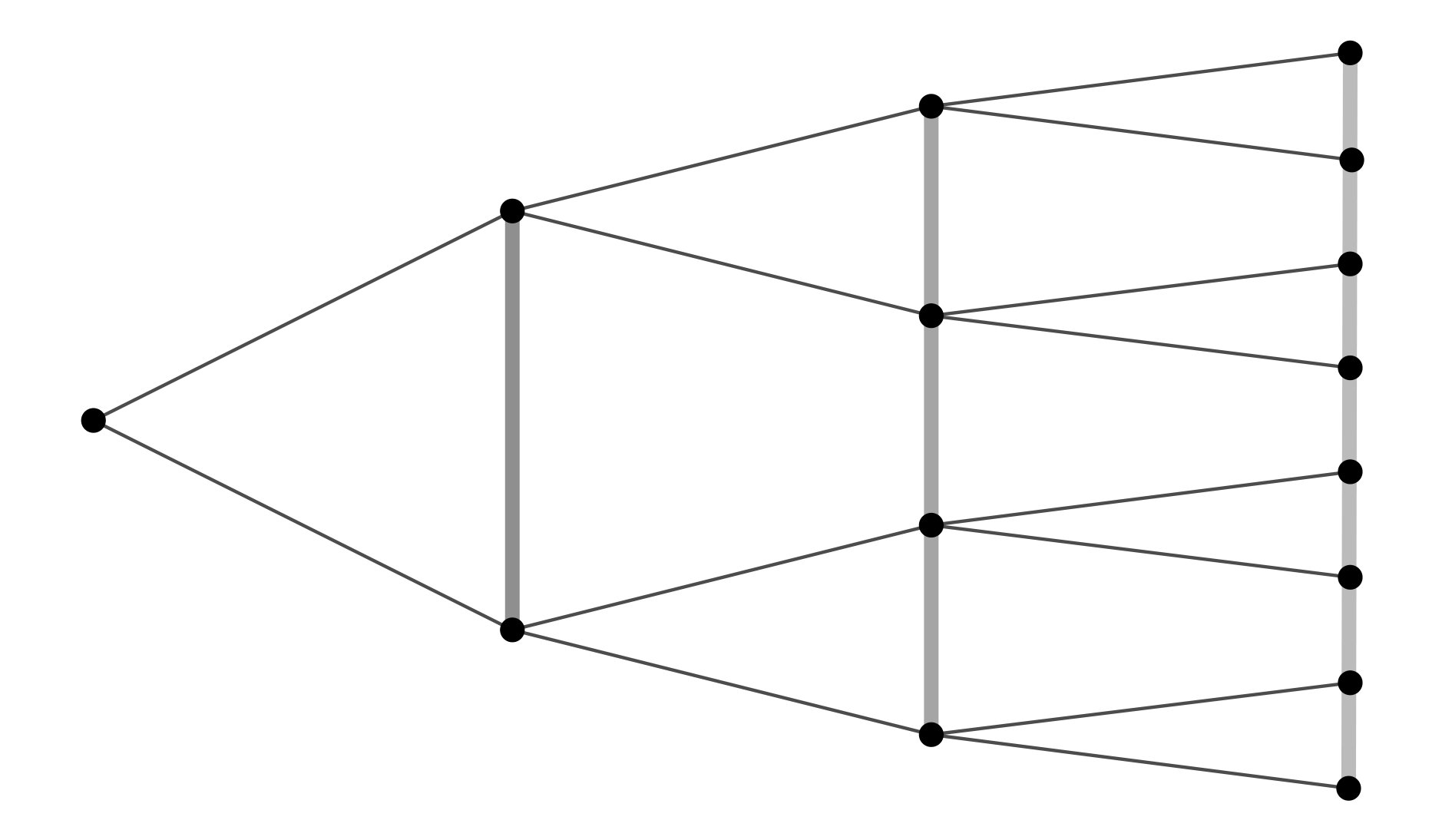 Figure 1
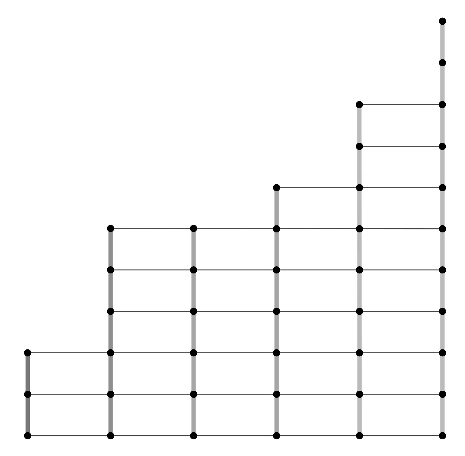 Figure 2
Peer Reviews
No public reviews on file for this paper yet. If you reviewed it on a platform where reviews are public (OpenReview, ICLR, NeurIPS, ICML), you can paste yours below so the community can read it here.
Videos
No videos yet. Explain this paper in a talk, walkthrough, or lecture? Add one.
Transfer matrices for discrete Hermitian operators and absolutely continuous spectrum
Christian Sadel
Facultad de Matemáitcas, Pontificia Universidad Católica de Chile
Abstract.
We introduce a transfer matrix method for the spectral analysis of discrete Hermitian operators with locally finite hopping. Such operators can be associated with a locally finite graph structure and the method works in principle on any such graph. The key result is a spectral averaging formula well known for Jacobi or 1-channel operators giving the spectral measure at a root vector by a weak limit of products of transfer matrices. Here, we assume an increase in the rank for the connections between spherical shells which is a typical situation and true on finite dimensional lattices . The product of transfer matrices are considered as a transformation of the relations of ’boundary resolvent data’ along the shells. The trade off is that at each level or shell with more forward then backward connections (rank-increase) we have a set of transfer matrices at a fixed spectral parameter. Still, considering these products we can relate the minimal norm growth over the set of all products with the spectral measure at the root and obtain several criteria for absolutely continuous spectrum. Finally, we give some example of operators on stair-like graphs (increasing width) which has absolutely continuous spectrum with a sufficiently fast decaying random shell-matrix-potential.
Key words and phrases:
Operators on graphs, finite hopping operators, spectral measure, absolutely continuous spectrum, extended states
2010 Mathematics Subject Classification:
Primary 47A10, Secondary 60H25, 82B44, 47B36
Contents
-
2.2 Some models with random decaying shell-matrix potential.
-
B Existence of absolutely continuous component in weak limits of measures
1. Introduction
1.1. The basic model
Let be some countable set and let be a (possibly unbounded) symmetric operator on with locally finite hopping. Locally finite hopping means that for any the set is finite where is the scalar product of (which will be anti-linear in the first and linear in the second component here) and is the unit vector in with and for . A large group of discrete models fall into this category, in fact any finite range hopping Schrödinger operator on any locally finite graph like is of this type. Because of the locally finite hopping condition, extends naturally to an operator on the set of all functions from to , . The natural and maximal domain of is then given by all functions such that . For the spectral theory we will later assume that is self-adjoint with this maximal domain.
Part of the motivation for this work was the development of criteria for proving existence of absolutely continuous spectrum in higher dimensional models. A big open problem is the so called extended states conjecture for the Anderson model in with small disorder in dimensions. The fact that this important problem in Mathematical Physics is unsolved for decades emphasizes the need for developing such methods. The Anderson model on a general graph is given by a random operator on which is the sum of a graph -Laplacian or adjacency operator and a random potential which is independent identically distributed at each site. The general wisdom (but it may depend on the graph) is that for large disorder (large variance) and at the edges of the spectrum the random potential dominates the spectral structure and one has pure point spectrum and so called Anderson localization. There are two general methods to prove this, the fractional moment method [AM] and multi-scale analysis [FS, GK1, GK2]. The fractional moment method at high disorder works fine in graphs with a finite upper bound on the connectivity of one point [Tau]. For a long time the high disorder Bernoulli Anderson model on for could not be handled for a long time. However, recently the localization has also been shown in this case in and dimensions [Li, LiZ]. Existence of continuous spectrum for Anderson models at low disorder has first been proved for infinite dimensional hyperbolic type graphs like regular trees and tree-like structures [Kl, ASW, AW, FHS, FHS2, KS, KLW, Sa1, Sa2]. Using averaging effects for the potential, it has also been shown on special graphs with a finite-dimensional growth, so called anti-trees and partial antitrees [Sa3, Sa4]. The key point was a one-channel structure and the use of transfer matrices.
Inspired from the rather complicated form of the transfer matrices appearing in [Sa4] we generalize this method further in a way that it can be in principle applied to any locally finite hopping operator, including models on higher dimensional graphs like the Anderson model in . The main Theorem 1 is a generalization of a spectral averaging formula well known for Jacobi operators giving the spectral measure at the root as a limit of absolutely continuous measures involving an expression depending on transfer matrices. This formula can be found in the book by Carmona and Lacroix [CL, Theorem III.3.2 and III.3.6] and has been used for showing absolutely continuous spectrum for random one-dimensional models with fast enough decaying random potentials [KiLS, LaS]. A generalization of this formula to one-channel operators is also a key point in [Sa3, Sa4]. Unlike in these cases, here we have to deal with affine spaces of rectangular transfer matrices at each level and products of such spaces where the dimension grows. However, re-interpreting the product of transfer matrices as a transformation of a natural partial semi-group structure (associativity) of boundary resolvent data permits a generalization of this formula. Furthermore, in this formula a maximum (or minimum in the denominator) for the choices of the transfer matrices within the affine spaces appears so that in principle one could try to find some specific choice to prove that a measure smaller than the actual spectral measure contains some absolutely continuous part. Then, the actual spectral measure will also contain some absolutely continuous part (cf. Theorem 3, Theorem 4 ).
Whether this method can be used to solve the extended states conjecture remains to be seen as hard estimates on resolvents have to be done and a good choice of the transfer matrices has to be found. But we expect it to be usable for Anderson type models in between the antitree and the case to approach the open problem and state the difficulties more precisely. As an immediate application we give a Last-Simon type proof [LaS] for absolutely continuous spectrum for random decaying shell-matrix potentials connecting one-dimensional wires, where the number of wires can be increasing and go towards infinity (cf. Theorem 5). This is already a non-one-dimensional problem and one has some (random) stair-like graph. As a by-product we also obtain the result for random decaying potentials on the strip as in [FHS3] (cf. Theorem 7). We also obtain absolutely continuous spectrum for random decaying shell-matrix potential on the Bethe lattice as a corollary (cf. Theorem 6). This may seem weak as the Anderson model with iid potential (diagonal shell potential) as a.c. spectrum, however, the statement includes radially symmetric potentials where the whole model is equivalent to a sum of one-dimensional Jacobi operators and the decay is really needed.
Let us emphasize that the transfer matrix method for one and quasi-one dimensional models has been extremely fruitful in the past. For instance, by analyzing the transfer matrix cocycle the global theory for one-frequency quasi-periodic Schrödinger operators on with analytic potential has been developed by Artur Avila [Avi] which was a major part for his Fields medal. Many abstract general theorems relating the asymptotic behavior of transfer matrix products to spectral theory can be in some way linked to the spectral averaging formula mentioned above. Therefore, we believe it can be a fruitful research program to revisit these relations and try to generalize such theorems using the spaces of transfer matrices as set up in this paper.
1.2. Quasi-spherical partitions, radial structure
Let be a symmetric operator on with locally finite hopping as described above. We may think of as a graph where are connected if and only if . Furthermore, let us assume that is connected with this graph structure, otherwise is an orthogonal sum of the operators on the connected components and we can reduce to one of them. We will use the set up as in [Sa4] and use a quasi-spherical partition, this means we partition into shells such that
[TABLE]
and
[TABLE]
We also define the sub-graphs
[TABLE]
This means connects only to and . If with the graph structure from as described above is connected, then a possible way to obtain such a partition is to take the spherical partition where is the -th sphere around some origin and denotes the graph distance111minimal number of edges passed when going from one point to another. For a standard Schrödinger operator in with the discrete Laplacian (graph adjacency operator) and some potential this leads to .
Choosing an order for all points in we identify and using primarily the order of the shells we identify with . For we have canonical isometric embeddings
[TABLE]
Its adjoints , are the natural projections from onto o .
We define the partial operators or partial Hermitian matrices on , the Hermitian matrix potentials and the connection matrix by
[TABLE]
Note that is a Hermitian matrix. The rank
[TABLE]
is at most the minimum of and . In lattices using the spheres as mentioned above, we find that is non-decreasing and is the maximal possible rank. However, one can use other decompositions and group together several spheres to one new shell in which case will not be maximal.
The polar or Hilbert-Schmidt decomposition of is given by where and are partial isometries, and is diagonal and invertible with the non-zero singular values of along the diagonal. Here, we use the notation for a matrix with values in where or . By putting the singular value part to the left or right (or possibly splitting it partly to and partly to ) and introducing some (conventional) minus sign we may write
[TABLE]
are all matrices of full rank. For example, we could choose and . However, the transfer matrix technique and formulas we develop will in fact work for any decomposition of this kind.
Note that and are not defined in this process (they do not appear as we do not have a st shell). We may select some root point and let be the normalized vector supported on . Or, we may also select some other non-zero root-vector . In any case, we select so that is a matrix of full rank which can be seen as a vector. In analogy of the notion of channels for strip-operators and the one-channel operators we may refer to as the backward channels at the -th shell connected to and as the forward channels at connected to .
Using the direct Hilbert sum structure given by the shells
[TABLE]
we write as direct sum
[TABLE]
Then, by (1.1) and (1.2) we find with the convention that
[TABLE]
1.3. Boundary resolvent data and transfer matrices
We define the to boundary data, , at the spectral parameter by
[TABLE]
Note that (or its column vectors) represent the modes connecting and therefore also to where as represents the modes connecting to the next shell . just represents the natural embedding of into meaning that we consider the column-vectors of and now as vectors in for obtaining the resolvent data . This means, is a matrix and is a matrix, similarly is a matrix. Hence, is a matrix and we assign to it its natural splitting and define
[TABLE]
by
[TABLE]
This means, e.g., that . Also note the general relations
[TABLE]
For we have the -th shell boundary data
[TABLE]
For some one may define by analytic extension of . Therefore, we define the first set of singular spectral parameters by
[TABLE]
So for the matrix exists. Clearly, is a subset of the eigenvalues of and therefore finite. We will make some additional assumptions:
**Assumptions:
(A1):** is non-decreasing,
(A2): We assume that for all and almost all real we have that the matrix has full rank .
The condition (A2) in principle says that the matrix connects all modes of and . This will be the case for typical operators like Schrödinger operators (adjacency+potential) on a connected graph. In fact, if has full rank for some real , then by considering the rational function we see that it has full rank for all but finitely many . The condition (A1) can always be obtained after grouping shells together. If the of is bounded one can group shells together such that the rank is (eventually) constant222one has a sub-sequence with and one can define new shells (defining ) to get a partition of with property (1.1) and ranks .. This is particularly the case for strip-like structures, but also for anti-trees. Otherwise, one can group the shells such that is increasing. Now, if one groups together up to (with ), then one needs for any in order to have a chance of fulfilling (A2). But the grouping can always be done in this way.
Under assumptions (A1) and (A2) we define
[TABLE]
With the assumptions above we immediately get that all are finite sets. We will show that any set is also finite. We call the set of singular parameters at the shell . In the work on one-channel operators [Sa4] we had for all and , and so on where numbers. In this case the transfer matrices featured some inverse of . As we have rectangular shaped matrices here, we need to make some different sense of this inverse. If is of full rank, then because there exists an affine space of right-inverses which we denote by , similarly we define .
[TABLE]
where denotes the unit matrix. We furthermore define
[TABLE]
If is invertible, then one simply has as sets, but if is not invertible (extreme case ) then may be a bigger set. In fact, if and is the space of matrices where each column vector is in the kernel of , then and . All these sets are well defined for and are defined for . In analogy to the transfer matrix formulas for one-channel operators in [Sa4] we define the sets of transfer matrices for by
[TABLE]
Note that is an affine subspace of , the set of matrices. We also define some simpler affine subspaces for by
[TABLE]
Furthermore, for we define the set of boundary vectors at with initial Dirichlet condition
[TABLE]
as well as the set of vectors with initial von Neumann condition
[TABLE]
Recall that and therefore are sets of matrices.
Remark 1**.**
(i)* Let us quickly note, that these matrices are a generalization of the transfer matrices for block-Jacobi operators. For instance, take on with finite, and an operator of the form*
[TABLE]
Then, for we can select and as well. This leads to for and there is only one choice, and leading to
[TABLE]
*which is the standard -th transfer matrix for such a block Jacobi operator. Only for we would have some different set of transfer matrices, depending on the selection of the vector .
(ii) Let us also note that the transfer matrices appearing as products in [FHS] are elements of these defined sets of transfer matrices. More precisely, there we have the special choices and for all , which are supposed to be full rank so that exists, giving . Then, choose and giving the special transfer matrix and we find*
[TABLE]
For subsets of matrices we denote if the matrices can be multiplied this way. We now define some further sets of singular spectral parameters. For let
[TABLE]
which is a finite set. This can be easily seen as the determinant is a non-zero rational function as for the inverse
[TABLE]
exists, using and where is the imaginary part in the algebra sense.
Proposition 1.1**.**
*Under assumptions (A1) and (A2) we have the following:
(i) For all , the set is finite.
(ii) For , and we find and*
[TABLE]
as well as
[TABLE]
(iii)* Particularly, we find for , that*
[TABLE]
(iv)* For fixed and all but finitely many we have*
[TABLE]
Before coming to the spectral theory, let us mention that we have some symplectic structure as in the Jacobi case.
Definition 1**.**
First, by we denote the standard symplectic matrix, this means
[TABLE]
where denotes the unit matrix, as before. We define the Hermitian-symplectic partial semi-group and the symplectic partial semi-group by
[TABLE]
Note, if or are such that one can multiply with from the left, then or as well. Note, is the Hermitian-symplectic group, is the complex symplectic group and is the real symplectic group of matrices.
For Jacobi and block-Jacobi operators it is well known that we have a symplectic structure for the transfer matrices. Here, there is something similar:
Proposition 1.2**.**
(i)* For we have . Moreover, for any we find .
(ii) If all and all and for are real matrices, then we have for that . Moreover, for any we find .*
Remark 2**.**
If we have a real operator , then are real and we can choose all to be real valued. In this case, for real energies the transfer matrix sets are subsets of . Now, as mentioned above, the square matrices in this set are part of a real symplectic group and particularly real. In the non-square matrices are not necessarily real. However, in this particular case, it would be sufficient to restrict to the set of real transfer matrices.
Like in the Jacobi case and the one-channel case there is also a connection to solutions of the formal eigenvalue equation. However, we need to exclude a further set of spectral parameters which is when for some . So on the real line we do not have any additional exclusions.
Proposition 1.3**.**
(i)* Let and let be a formal solution of , i.e. for and with . Assume that or . Then, there exist , , such that*
[TABLE]
In particular, we find
[TABLE]
(ii)* Let , let be given a vector and a selection of transfer matrices . Then, there exists a formal solution of such that*
[TABLE]
Note, the correspondences in and are not one-to-one in general! If we let , then is a formal solution of and one can relate to as some form of ’boundary condition’.
2. Main Results
2.1. Spectral Theory
So far, everything can be well defined for unbounded symmetric operators with local finite hopping. For spectral theory we need a self-adjoint operator. As mentioned above, we want to be self-adjoint with its maximal domain.
Definition 2**.**
A Hermitian (possibly unbounded) operator on with locally finite hopping will be said to be self-adjoint with its natural domain, if the set of compactly supported vectors, , is a core for , i.e. is essentially self-adjoint.
has the maximal possible domain in terms of restricting (as operator on ) and its range to , i.e. the domain of is given by all functions in such that is as well in . This is the natural domain for in . Note that is essentially self-adjoint if and only if is self-adjoint in which case is a core. In the language of physicists this property means that one does not have to specify a ’boundary condition at infinity’. It is evident that operator-norm bounded operators have this property. From now on by we consider the operator with its natural domain, i.e. .
If is self-adjoint then we will denote the spectral measure at the chosen root-vector by , i.e.
[TABLE]
Theorem 1**.**
Assume that is self-adjoint with its natural domain and that assumptions (A1), (A2) hold. There is a point measure supported on and generated by compactly supported eigenfunctions of , such that
[TABLE]
where denotes the Lebesgue measure in and the limit has to be understood in the weak topology of finite Radon-measures (i.e. iff for bounded continuous functions ).
Note that this is a generalization of [CL, Theorem III.3.2], [Sa3, Theorem 2.3(iii)] and [Sa4, Theorem 2(i)]. As in the cases before, the proof uses some spectral averaging technique in the -th shell for the operator (restriction to the of to ) which selects a certain point within the Weyl discs. Then, the limit point property in the case of self-adjointness reflects the fact that the averaged spectral measures converge to the actual spectral measure of for . Here, we have the following Weyl discs:
Theorem 2**.**
Let let the -th Weyl disc be given by
[TABLE]
where denotes the ’imaginary part’ of in algebra sense and denotes the topological closure of a set . Assume that assumptions (A1) and (A2) hold, then:
- (i)
* is a closed (circular) disc in the upper half plane, and is either a closed limit disc with positive radius (limit circle case) or it consists of only one point (limit point case).* 2. (ii)
If one of the deficiency indices is zero (particularly if is self-adjoint) then consists of one point. If is self-adjoint, then
[TABLE] 3. (iii)
Let . Then, is a limit disc of positive radius if and only if there are functions with and and .
Remark 3**.**
(i)* For semi-infinite Jacobi operators (semi-infinite tri-diagonal Hermitian matrices) it is well known that the limit point property is equivalent to being self-adjoint. Furthermore, in the case where is a limit disc, each point on the boundary (the limit circle) characterizes a self-adjoint extension of . A nice proof of these facts from the discrete analogue of Weyl-Titchmarch theory can be found in Techl’s monograph on Jacobi operators [Tes]. For one-channel operators we have shown the equivalence under certain conditions, for instance, if all matrix entries of are real [Sa4].
(ii) One might work with some matrix (using ) consisting of column vectors in and Weyl-discs (with same formula as above) of higher dimensions where one can have different types of limit discs (different dimensions). In the case of Jacobi operators with matrix entries (operators on strips) this is a typical choice to get the usual transfer matrices. The Weyl-Titchmarsh theory in this case is developed in [Ber] and for the nice geometric picture of these higher dimensional Weyl discs see [Fuk, Sch].*
Theorem 1 gives the following useful criteria. By , we denote the spectrum and the absolutely continuous spectrum of as closed sets.
Theorem 3**.**
(i)* Let be given an interval . Suppose for some increasing sequence of positive integer and all there is a measurable function , such that*
[TABLE]
*Then, meaning that the measure has an absolutely continuous part whose support contains . In other words, there is absolutely continuous spectrum everywhere in .
(ii) Suppose that we find some almost everywhere positive, locally integrable function and measurable functions such that for any compact set of positive Lebesgue measure we have*
[TABLE]
Then, , i.e. there is absolutely continuous spectrum everywhere in .
Part (ii) is using the criterion of Deift-Killip [DK] in their work on absolutely continuous spectrum for Schrödinger operators with potentials on . Now, with some stronger condition we get to pureness of absolutely continuous spectrum like in the criterion of Last-Simon [LaS].
Theorem 4**.**
- (i)
Suppose for some , and one finds measurable functions and such that
[TABLE]
Then, the positive measure (as in Theorem 1) restricted to is purely absolutely continuous with a density which is in . Hence, is purely absolutely continuous in . 2. (ii)
Suppose for some , and one finds a measurable function such that
[TABLE]
then and the measure is purely absolutely continuous in with an density. Hence, is purely absolutely continuous in and there is spectrum.
Remark 4**.**
Note that in all the theorems one may construct by selecting for each and taking the product . In Theorem 4 (i) we do not get existence of spectrum. Particularly, for Jacobi operators on the half line one finds such for in the resolvent set where the measure is zero. But as is in fact an absolutely continuous measure, there is no contradiction here.
2.2. Some models with random decaying shell-matrix potential.
As a first application for random models we will obtain a Last-Simon type of proof for absolutely continuous spectrum for a random decaying shell-matrix potential which couple an increasing number of wires. By shell-matrix potential we mean a direct sum operator with being a Hermitian matrix and . Let be given a sequence of natural numbers with and let
[TABLE]
Furthermore let be given a sequence of real numbers with . Then we define the free operator on by
[TABLE]
for where if or and . This operators describes independent wires at different mean energies for the -th wire. Moreover, the -th wire starts at the -th shell where . After the coupling with this becomes a stair-like structure. Let be a random Hermitian matrix, that is a Hermitian matrix valued random variable defined on some abstract probability space . We assume that are independent and
[TABLE]
where we use the standard matrix norm in any and denotes the expectation value, that is . Then, we consider the random operator
[TABLE]
where we identify . Let us consider
[TABLE]
which is not empty by the assumption on the above. In terms of a graph structure (applying an edge from to whenever ) the graph looks stair-like, the horizontal lines come from the basic operator and the vertical stripes symbol random graphs with random edge-weights coming from the , where the ’strength’ of is decaying.
Theorem 5**.**
Almost surely, the random operator has purely absolutely continuous spectrum in i.e. for -almost all ,
[TABLE]
where denotes the absolutely continuous spectrum, the pure point spectrum, and the singular continuous spectrum of , respectively (as closed sets).
Remark 5**.**
Note, that in the non-random case ( is constant in ) the condition (2.1) looks trace-class like, . However, since can grow towards infinity arbitrarily fast, it does not imply that the shell-matrix potential is actually trace class.
With a unitary conjugation a similar result follows for the Bethe lattice. Therefore, let be the rooted binary Bethe lattice (or binary tree). is constructed the following way: there is some root being the zeroth generation and then each point in the -th generation is connected to two ’children’ in the st generation.
We let the -th shell denote the set of points in the -th generation (graph-distance from the root). Then, we have and we let be a random sequence of Hermitian matrices as above satisfying (2.1). Like above, is the part of in the -th shell. We let be the negative adjacency operator on and define as above,
[TABLE]
For we have again that . With we denote the smallest integer which is bigger or equal to . In terms of a graph structure it looks like this, where again the vertical stripes are random graphs describing .
The spectrum of is absolutely continuous and given by the interval . In the interior we find absolutely continuous spectrum of .
Theorem 6**.**
Almost surely, the random operator has purely absolutely continuous spectrum in , that is to say that almost surely,
[TABLE]
and
[TABLE]
Another special case of Theorem 5 gives a result on random decaying matrix potentials on a strip. For uniform compactly supported matrix potentials this result has been already proved in [FHS3]. Therefore, let be the product graph of a finite graph and the half-line , hence and we choose and may use . Then, a vector in is given by a sequence with where . The unperturbed Laplacian on is given by
[TABLE]
where formally and is some basic Hermitian adjacency or Laplace operator on the graph , possibly complex (with magnetic phases). Let have the eigenvalues , then the spectrum of is given by the union of bands:
[TABLE]
We will also consider the intersection of the open bands as before
[TABLE]
Then, as before, we add a random, independent, decaying matrix potential satisfying (2.1) and consider the random operator given by
[TABLE]
Theorem 7**.**
(i)* The random operator has, almost surely, purely absolutely continuous spectrum in the intersection of the open bands , that is, for -almost all ,*
[TABLE]
(ii)* Almost surely, , that is, the absolutely continuous spectrum of is equal to the union of bands which is also equal to the essential spectrum of , almost surely.*
Remark 6**.**
(i)* Note that the result is actually slightly more general than [FHS3] as they have the additional assumptions that the distribution of all matrix potentials is supported in one compact set . Under these additional assumption, the bound follows automatically from .
(ii) We do not prove pure absolutely continuous spectrum in part (ii). As a set, the essential spectrum and the absolutely continuous spectrum are the same. We expect the absolutely continuous spectrum to be pure away from (internal and external) band edges. This will be dealt with elsewhere.*
3. The algebra of the boundary resolvent data
We want to consider the partial semi-group structure associated to the boundary resolvent data. For this reason we introduce the following binary operation between suitable matrices.
Definition 3**.**
- (i)
We let denote the set of matrices with the assigned splitting. Such a matrix will be considered as a collection of 4 blocks (matrices) of size , , and . This means,
[TABLE] 2. (ii)
Let and with the corresponding splittings
[TABLE]
We say that the ordered pair is suitable if is invertible (in which case also is invertible) where denotes the identity matrix.
If is suitable then we define
[TABLE]
by
[TABLE]
The index indicates that the operation does in fact depend on the splitting of the matrices and and particularly on , the size of the second assigned diagonal block of or the first diagonal block of . If the blocks are clear we may omit the index . 3. (iii)
Furthermore, we define the following subset of
[TABLE]
where denotes the imaginary part in the sense of algebra operations for square matrices . Similarly, we let .
We use this operation for going forward along the shells in the graph. The symbol shall indicate this radial move going from a lower shell in the graph outward, cf. Proposition 3.2.
Proposition 3.1**.**
(Associativity)
- a)
Let be given a matrix , a matrix and an matrix . Then, if all the appearing combinations below are suitable, then
[TABLE]
and therefore we may define this to be . If the splitting of is clear, we may simply write . 2. b)
If , then is suitable and . Particularly, \big{(}\bigcup_{q,r}{\mathcal{M}}(q,r,\pm),\triangleleft\,\big{)} are partial semi-groups.
Before coming to the proof of this proposition, let us state the main fact for this definition.
Proposition 3.2**.**
For , and all we have
[TABLE]
Furthermore, for , , we have
[TABLE]
The crucial parts of these propositions come from the following Lemma.
Lemma 3.3**.**
Let and be invertible matrices, , , and such that
[TABLE]
and let be suitable, then
[TABLE]
if the occurring inverse exists.
Proof.
Let
[TABLE]
where denote the Schur complements
[TABLE]
Furthermore, let
[TABLE]
Using the resolvent identity we obtain for ,
[TABLE]
where the inverses exist because and are -suitable. Then,
[TABLE]
and furthermore
[TABLE]
These equations correspond exactly to (3.1). Analogously, one obtains (3.2) as well. ∎
Proof of Proposition 3.1.
Part a). We can use Lemma 3.3 twice in different ways to get
[TABLE]
For the left equation we use and . For the right equation we use and . Formally, this calculation only proves the identity if all the appearing inverses and particularly and exist. By continuity we get the statement in general.
For part b) we use the same notations as above in Definition 3. Note first that and implies and therefore exists. This implies that and are -suitable.
Now, for the case we can use Lemma 3.3 with , to see immediately that . By continuity we get for and . Consider the matrix
[TABLE]
We claim . Indeed, is clear by and . Assume
[TABLE]
Because and this implies and thus which immediately gives as . Thus and . Using the Schur complement formula and (3.1) we see that
[TABLE]
Similarly one proves . ∎
So finally we use Lemma 3.3 to prove the important Proposition 3.2.
Proof of Proposition 3.2.
The first statement is clear by definition as and are matrices of full rank equal to the number of columns. Only note that for the matrix may not be of full rank and therefore the imaginary part of may not be strictly positive.
Now, let denote the maps and with the natural extension of the image set to which means and . Similarly, we denote by the natural extensions of and with the image set extended to . Furthermore, let , . Then, we have exactly the situation as in Lemma 3.3 with where is defined as in the proof of Lemma 3.3. Thus, the lemma gives the result directly. ∎
4. Transformation to matrix multiplication
A simple, natural partial semi-group structure is given by matrix multiplication (of rectangular matrices). Thus, it is a valid question whether one can transform the operation into a matrix multiplication. In fact, considering one-channel operators one has a particular transfer matrix structure coming from the resolvent boundary data. The form of these transfer matrices leads to the definitions (1.11), (1.12), the only subtlety is that now is not necessarily a square matrix and the inverse of appearing in [Sa4] makes no immediate sense. Still, working with right-inverses, Proposition 1.1 can be seen as transforming the relation of Proposition 3.2 into multiplication of sets of matrices. The main focus of this section is the proof of Proposition 1.1 and we will also obtain Proposition 1.2.
In analogy to the defined transfer matrices we may generally make the following definition.
Definition 4**.**
- (i)
For we denote by the set of matrices with assigned splitting where the upper right matrix part has full rank (that is to say that as a linear map is surjective), i.e.
[TABLE] 2. (ii)
Let and let denote the set of right-inverses to . Furthermore let . Then, we define the associated affine spaces of transfer-matrices
[TABLE]
and
[TABLE]
as well as the left and right-parts
[TABLE]
Note that and . The used notation is based on ’Dirichlet’ and ’von Neumann’ boundary conditions.
Remark 7**.**
If is invertible, then and one could replace for some . But if is not invertible, then one may only have .
Proposition 4.1**.**
Let , , so particularly . Assume and are -suitable, then and we have:
[TABLE]
In particular we find
Proof.
First, from (3.1) one immediately sees that is surjective and thus has maximal rank, so . We use the same notations for and as always (see Definition 3.ii ) and let
[TABLE]
where , , . Then, we need to show
[TABLE]
First, we have and using (3.1) we find . Then, we obtain
[TABLE]
So we get indeed that and hence . Clearly, and using the special case we get . By Proposition A.1 we get all right inverses of by varying and over all right inverses to and . Hence, which finishes the proof of the first statement. .
Considering , we get
[TABLE]
which gives
[TABLE]
Finally, we need to check that . We have that
[TABLE]
and
[TABLE]
So we see that the left hand sides of (4.3) and (4.4) are equal if and only if
[TABLE]
where we used . Let us transform the right hand side,
[TABLE]
Using (4.6) the right hand side of (4.5) becomes which is equal to the left hand side of (4.5). Thus, we proved and .
For equality in the second inclusion we first claim the following: For any fixed such that , for we get
[TABLE]
First, because is invertible, we get and therefore, by Proposition A.1 where . The limit gives the claim.333Note that for small but non-zero , is invertible. If is invertible, then and and we do not need this trick , however, if is not invertible this limit may give a bigger (higher dimensional) affine space as using .
Finally, for any element such that and some fixed as above, we have
[TABLE]
Thus, we find and such that
[TABLE]
and therefore, and we get . But in fact, we get the full set just by varying and for any fixed and . ∎
Now we obtain Proposition 1.1 basically as a corollary:
Proof of Proposition 1.1.
First, if then and are suitable and one can define by , so is well defined at least after analytic continuation. Moreover, is of full rank (cf. (3.1), hence, . This particularly gives . Since is finite and is always finite we get by induction that is finite for any (note ) proving part (i).
Proposition 3.2 and Proposition 4.1 give part (ii) as and . Using , part (iii) follows from (ii) as and . Part (iv) follows from (iii) by induction. ∎
Proposition 1.2 follows directly from the following.
Proposition 4.2** (Symplectic structure).**
*Let , .
(i) If is Hermitian, , then , that means is a set of (rectangular) Hermitian-symplectic matrices. Moreover, for any we find .
(ii) If is symmetric (in matrix sense), , then , that means, is a set of (rectangular) symplectic matrices. Moreover, for any we find .*
Note that generally are sets of rectangular matrices, so we do not talk about elements of the Hermitian-symplectic or symplectic group, we rather talk about elements in the partial semi-groups as defined in Definition 1.
Proof.
Using our standard notations, implies , and . Let , we find
[TABLE]
where we used and . Using this shows . The second part,starting with , follows by the same calculations replacing by the transpose everywhere. ∎
5. Relation to formal solutions of the eigenvalue equation
The main point of this section is to prove Proposition 1.3. The first part, Proposition 1.3 (i) states the following: If we have for a formal solution of , then, there exist , , such that
[TABLE]
In the second part it is stated that for any solution of the transfer matrix equation with any choice of transfer matrices there is also a corresponding formal solution satisfying the equations above. Let us start with the following lemma.
Lemma 5.1**.**
Let , then for any we have .
Proof.
For we have that exists. Hence, let and let
[TABLE]
Then, implies so that the second equation gives . For the kernel of is just the zero vector so that which implies and finally . Hence, the kernel of consists of only the zero vector. ∎
Proof of Proposition 1.3.
Let be a formal solution of . Moreover, let , , and . Under the assumption that (meaning it is not the zero vector) we will prove the existence of such that . For this is fulfilled by assumption and by Lemma 5.1 we obtain that . Hence the existence of for any then follows by induction.
So let . By the assumptions together with (1.5) we have
[TABLE]
Assume for a moment that is invertible. Then by applying the inverse on both sides and multiplying by or from the left we obtain
[TABLE]
As we have that is defined at least by analytic continuation, so the kernel of is orthogonal to the column vectors of and . Hence, one may project to the subspace in orthogonal to the kernel of . Then, applying the inverse to (5.1) in this subspace also gives (5.2).
Now take some and let . By the first equation of (5.2) we get , thus, . Let denote the set of matrices where each column vector is in the kernel of . Now, if , then at least one entry is not zero and one can create a matrix which has all column vectors equal to zero except for one, such that , moreover, we let .
If then by assumption and we find such that and we let in this case. Then, in either of the cases, we find for and that
[TABLE]
Plugging this into the second equation of (5.2) gives
[TABLE]
Together, this means
[TABLE]
In part (ii) of Proposition 1.3 we have the reversed situation: For some we are given some transfer matrices and a starting vector and we want to construct a corresponding formal solution to . Therefore, define
[TABLE]
It easy to check that satisfies the equations (5.2). If is invertible, then we define
[TABLE]
for any . If is not invertible, then all the column vectors of and are orthogonal to the kernel of because exists by analytic extension. Hence, we can restrict to the orthogonal complement of the kernel and take the inverse there. This way, is always well defined. It is clear that satisfies (5.1) and with (5.2) we find and for . Both together give that is indeed a formal solution of . ∎
6. Weyl discs and limit point property
In this part we prove Theorem 2 and prepare for the spectral averaging formula leading to Theorem 1. Let us first introduce some notations. The set of unitary matrices will be denoted by , the disc of matrices with singular values smaller equal to one by , the set of Hermitian matrices by , the set of matrices with non-negative imaginary part by and . This means
[TABLE]
[TABLE]
Recall that is the imaginary part in the sense of algebras, meaning that real and imaginary part are Hermitian matrices.
Let us consider the partial operators on . We will view and the column vectors of as vectors in and simply write and . Recall that with this convention we have
[TABLE]
For , meaning , and let us define
[TABLE]
Note that are matrices and hence, just numbers in the upper half plane for . In analogy to Weyl circle and Weyl disc for Jacobi operators we define the following.
Definition 5**.**
For the -th Weyl region* and the -th Weyl disc are defined by*
[TABLE]
where denotes the closure of a set (this amounts to formally allowing to have infinite values.)
The standard resolvent identity yields
[TABLE]
Since , the inverse is well defined for .444Indeed and assuming we get . The imaginary part of the right hand side is lower or equal to zero, and of the left hand side it is larger than zero, unless . Hence, in which case . Also, we see that the Weyl disc as defined here is the same as in Theorem 2.
Proposition 6.1**.**
*Let , then, we have the following:
(i) is a compact, closed disc in the upper half plane. If then is the surrounding circle, if , then .
(ii) Let and let be the set of all formal555By formal solutions we mean that we consider the space of all -sequences and not only . solutions of with . Then, the radius of the Weyl disc satisfies*
[TABLE]
(iii)* .*
Proof.
Let , , and, moreover . Note, gives and when is invertible. Using continuity and density of invertible matrices it is sufficient to consider invertible matrices in the definition of and and by (6.2) one finds
[TABLE]
Thus, and are affine projections of and under the same affine map. Note that
[TABLE]
can be regarded as a generalized Möbius transform acting on . Similarly as the Möbius transforms in the upper half plane it maps generalized ’circles’ and ’discs’ into such ’circles’ and ’discs’ where generalized circles are Möbius transforms of the unitary group and generalized ’discs’ are such images of . Here, we will give some direct calculations. Let . First, we show the following.
[TABLE]
Clearly, by redefining , the set is given by . Now, equating this expression in with the one in in the claim gives the relation
[TABLE]
For such is well defined. Then,
[TABLE]
Therefore, becomes equivalent to
[TABLE]
which is indeed fulfilled.
On the other hand, having we can define and the calculation above shows for . This gives claim 1.
The above relations also directly give a one to one correspondence between and as well as between and . Thus, we obtain directly that
[TABLE]
and are of the form with , being a complex row vector, a complex column vector and varying in or , respectively. For we see immediately that is a disc in and the boundary circle and the same is true for and . For both represent the same disc:
[TABLE]
Changing with where are adequate unitaries, we can assume that and are multiples of , the first canonical basis vector in . This means and are given by where , is the top left entry of the matrix and varies in or , respectively. It is a well known fact of linear algebra that for we find
[TABLE]
This shows that is indeed a closed disc and .
For part (ii) note that from the formulas above the representation gives the radius
[TABLE]
We first prove:
[TABLE]
Let us use the notation for . Then from we have
[TABLE]
Using this gives and thus
[TABLE]
as well as
[TABLE]
Now, and, therefore, using Cauchy-Schwarz we get
[TABLE]
Now, using Proposition 1.3 one finds such that
[TABLE]
which gives equality above and proves Claim 3. Note that for the row vector is not zero and as we are not dividing by zero. Realizing that one finds similarly
[TABLE]
Together with Claim 3 and (6.3) this proves part (ii).
For part (iii) note that by Proposition 3.2 and (3.1) we find
[TABLE]
Formally varying the matrix-potential (which changes ) then shows which by (i) implies . ∎
Now, as we see from (iii), the radius of the Weyl disc is shrinking and we can define which is the radius of the limiting disc . If then the intersection consists of one point and we have a limit point. If then we have a limit disc.
Proposition 6.2**.**
(i)* Let . We have a limit disc, , if and only if there exist and . In particular, in this case both deficiency indices are at least one, .
(ii) If is self-adjoint on its natural domain, then we have the limit point case and for any sequence we find*
[TABLE]
and thus,
[TABLE]
Proof.
If and exist then Proposition 6.1 (ii) immediately gives .
Now let . Then by Proposition 6.1 (ii) you find such that
[TABLE]
for . Now, take for and for . This way, for all . Then, there is a weakly convergent sub-sequence . In particular, for any . Using continuity in the eigenvalue equation we find . Note, with , and hence . The same arguments hold for replaced by .
For part (ii), if is self-adjoint with its natural domain, i.e. the compactly supported vectors form a core, then (which act as zero in ) converge to in strong resolvent sense666Indeed, for it is obvious that and if is a core, then this implies strong resolvent convergence for any choice of as . This immediately implies the result. ∎
Note that Proposition 6.1 and 6.2 prove Theorem 2.
7. Spectral averaging formula
We let
[TABLE]
denote the standard Cauchy distribution on . The Cauchy distribution can be obtained as the pull back measure of the standard Haar measure on the unit circle by the Caley transform,
[TABLE]
as a map from to . Then we define the -th level averaged spectral measure at by
[TABLE]
that is we consider real diagonal matrices only and integrate the spectral measures over the product measure of the Cauchy distribution on the diagonal entries.
If is a complex analytic function on the upper half plane and continuous up to the boundary and at infinity, then Cauchy’s formula gives
[TABLE]
Note that
[TABLE]
is of this form in each diagonal coordinate of . Therefore, the Stieltjes transform of is given by
[TABLE]
The limit point property in the case where is uniquely self-adjoint gives which reflects the fact that weakly for .
Proof of Theorem 1.
The key for proving Theorem 1 is to obtain the density of the spectral averaged measures and identifying its singular part. For this we consider the Stieltjes transform
[TABLE]
For the limit for exists. Thus, the singular part of is supported on the finite set and given by a point measure . The absolutely continuous part of has the density (Radon-Nikodym derivative with respect to the Lebesgue measure )
[TABLE]
where denotes the real part of a matrix in algebra sense and we define
[TABLE]
We used the facts that , is a real number and is Hermitian (note ). Also note that is indeed a matrix and hence a vector in . Now assume , let and consider
[TABLE]
Then, and . Thus, the Cauchy-Schwartz inequality gives us
[TABLE]
Using and we get equality, therefore
[TABLE]
Thus,
[TABLE]
Note that this is a generalization of the spectral averaging formula [CL, Theorem III.3.2].
Now let us consider the singular part of closer. We already know that it is supported on which is finite and hence it is a point measure. As the Cauchy distribution is absolutely continuous we see that for if and only if has positive (Lebesgue) measure. It is a well known linear algebra fact (using Fubini and rank-one perturbations) that this can only occur if there is an eigenvector which is orthogonal to all column vectors of and has some overlap with . This means that , and . This in fact implies that is an eigenvector of for any . Moreover, only such eigenvectors contribute to . Hence, let
[TABLE]
be the part of the eigenspace of for which is orthogonal to the range777we interpret as a map from to of (orthogonal to all the column vectors of ). Let
[TABLE]
[TABLE]
From it also follows that any eigenvector is an eigenvector of for any and any , that is to say for any . Here, formally we have to consider the natural embedding of into . This immediately implies for that and . Hence, is a sequence of growing positive point measures which is bounded by and thus it converges to a point measure supported on . Moreover, any eigenvector is an eigenvector of (or better the formal embedding of into is) and is generated by those eigenvectors. This means, let
[TABLE]
be the closure of the union of the embeddings of into and let be the orthogonal projection. Then, where we now consider as an element in (that is , here). The convergence of gives
[TABLE]
where the limit has to be understood as a weak limit of finite measures. This proves the theorem. ∎
We like to remark that the measures and hence need not be zero. Already in the one-channel case there can be compactly supported eigenfunctions, cf. [Sa3, Sa4].
8. Criteria for absolutely continuous spectrum
In this section we will prove Theorem 3 and Theorem 4. First of all, we note that for any choice of matrices we find
[TABLE]
with as defined above. As this density appears through an average of spectral measures at over a probability distribution, we find
[TABLE]
and, hence, is a positive function for any measurable choice of . Moreover, any infimum over such a function is also in .
Proof of Theorem 3.
Part (i). We have
[TABLE]
On the right hand side we have an absolutely continuous measure with a positive density on by the assumptions of Theorem 3. Therefore, the bigger positive measure has to have an absolutely continuous part with a bigger support than . This means, .
To show part (ii) note that using the condition in the Theorem implies
[TABLE]
for any compact set of positive Lebesgue measure. Using the arguments as in [DK], or Proposition B.1, it follows that the limit measure has an absolutely continuous part everywhere in . ∎
Proof of Theorem 4.
By the arguments in the previous section we find a matrix such that
[TABLE]
From Proposition 1.2 we find
[TABLE]
and for that reason
[TABLE]
It follows immediately for that
[TABLE]
Hence, there is a sub-sequence such that the norm of in is uniformly bounded along this sub-sequence. Using separability, reflexiveness and weak- compactness, we find a further sub-sequence which converges weakly in , i.e. . Then, integrating against bounded continuous functions in which are also in where , we see that
[TABLE]
and hence in the interval . This proves part (i). Part (ii) follows immediately from part (i) and Theorem 3 (ii). ∎
9. Application to random models
In this section we first prove Theorem 5 and then Theorem 6 and Theorem 7 will follow with little extra work. Thus, consider the operator .
Proof of Theorem 5.
The matrix-potential part of in the -th shell is given by
[TABLE]
We will use for , giving for . Furthermore we let be some normalized root vector, so that generally . Similar to Remark 1 (ii), the special choices and lead to the transfer matrices
[TABLE]
These choices lead to nice entire functions in .
Let us also note that if and , then, it follows inductively that for all (as the width is growing, ). Hence, there is no non-zero compactly supported eigenvector. Thus, the measure as in Theorem 1 is zero.
Claim: We have
[TABLE]
for any compact sub-interval of .
Using Theorem 4, the argument above, Fatou’s lemma and Fubini, it will follow888Indeed, this implies by Fubini and Fatou’s lemma and a bound in expectation implies almost sure boundedness to use Theorem 4 (ii). that the spectral measure at is purely absolutely continuous in .
So let us prove the claim. By sub-multiplicativity of norms, we can exchange and by and , respectively, where (with ) and , are uniformly bounded for and . Using the bound for any orthonormal basis in and any matrix , it is, thus, sufficient to prove
[TABLE]
for as above and all fixed .
For all values on the diagonal of the diagonal matrix are elements of and we may write for some real diagonal matrix with and . For the unperturbed operator (all ) the transfer matrices for are equal to
[TABLE]
and we define
[TABLE]
Using one obtains
[TABLE]
where depends on as well. This implies
[TABLE]
Note that is an isometry, , and for , the values are uniformly bounded away from and . Hence, and are uniformly bounded in and . Moreover, the random matrices are independent and satisfy a bound as in (2.1) uniformly in . We will now omit the dependence on in most calculations. Furthermore, we consider some starting vector and define
[TABLE]
Then, we find
[TABLE]
Squaring out the last term, taking expectations and using the independence of from we find
[TABLE]
For the terms only having one factor it is important to first do the expectation and afterwards the norm bound. Using and (2.1) we see that the product over of the terms in the bracket on the right hand side remain bounded, uniformly for . Hence, for we obtain is uniformly bounded in which implies the claim (9.1).
As explained above, this applies for any . Thus, the spectral measure at is almost surely purely absolutely continuous in , and there is spectrum.
Let us define the sub-graphs and let be the restriction of to . Again, using Theorem 5 will give that for any point the spectral measure at of the operator is, almost surely, purely absolutely continuous in . As is countable, we find a set of probability one, , such that for all and all , the spectral measure of at is purely absolutely continuous in . Combining this with a soft modification of [FLSSS, Lemma 2.2.] one obtains that the spectrum of is purely absolutely continuous in for all . ∎
The proof of Theorem 6 follows directly from Theorem 5.
Proof of Theorem 6.
Recall for the binary rooted tree we have {\mathbb{G}}_{2}=\big{\{}(n,j)\,:\,n\in\mathds{N}_{0},\,j\in\{1,\ldots,2^{n}\}\,\big{\}} and . We define the normalized symmetric and anti-symmetric mean-field vectors
[TABLE]
and we let denote the zero vector in . Then, we define the matrices
[TABLE]
It is not hard to check that is a unitary matrix and we can define the unitary operator on by
[TABLE]
Let for be defined by
[TABLE]
where denotes the -th canonical basis vector in . Hence, is simply th -th column vector of the matrix . Then it is not hard to check that
[TABLE]
where for or . Thus, considering the model on as above with the special case and for all we find
[TABLE]
Now, is a shell-matrix potential of the same type as where is replaced by . In particular, it also satisfies (2.1). Therefore, Theorem 5 gives that the spectrum of is almost surely purely absolutely continuous in , and there is spectrum. ∎
Now, Theorem 7 (i) can also be regarded as a special case of Theorem 5. The step from Theorem 7 (i) to Theorem 7 (ii) will then be done as in [FHS3].
Proof of Theorem 7.
Without loss of generality we may assume that is diagonal. If not, let be diagonalized by the unitary , that is , and consider , with . There, and are exchanged by and , respectively, which is another sequence of random Hermitian matrices satisfying (2.1). Hence, we let
[TABLE]
With this basis change we also see that is (unitarily equivalent to) a direct sum of one-dimensional operators where is an operator on given by the discrete Laplacian and a constant potential . It is well known that the spectrum of is purely absolutely continuous and given by the interval , so the spectrum of is given by the union of these bands. By (2.1), and the fact that is constant, the difference is a Hilbert Schmidt-operator (almost surely). Thus, the essential spectrum of is also given by , almost surely. Moreover, corresponds to of Theorem 5 with fixed width , with and corresponds to as above. Thus, Theorem 5 implies that, almost surely, the spectrum of is purely absolutely continuous in .
For part (ii), first consider a subset and define the canonical embedding . For the set is not empty. We also define and let . Then, we may write
[TABLE]
where denotes unitary equivalence. By Theorem 7 (i) has almost surely pure absolutely continuous spectrum in , and there is spectrum. By the considerations above on the essential spectrum of , has no essential spectrum in . As , the off diagonal terms only come from the random potential and are almost surely Hilbert-Schmidt operators from to and vice versa. Thus, using [FHS3, Theorem 6] we find that has almost surely absolutely continuous spectrum in all of (not necessarily pure). Noting that is dense in , part (ii) follows as almost surely. ∎
Acknowledgment
C.S. has received funding from the Chilean Fondo Nacional de Desarrollo Científico y Tecnolǵico (FONDECYT) 1161651 and the Iniciativa Científica Milenio through the Nucleo Mileneo MESCD on ’Stochastic Models of Complex and Disordered Systems’.
Appendix A Some linear algebra facts
As before with we define the set of matrices over where or . For with of full rank there exist right inverses, that is matrices such that where is the unit matrix.
Proposition A.1**.**
Let , of full rank and of full rank with or . Then is of full rank and the set of right inverses is given by the set of products of right inverses to and , i.e.
[TABLE]
Proof.
We can regard as a surjective linear map from to and as a surjective linear map from to . It is thus clear that is a surjective linear map from to and hence of full rank. We let denote the standard basis in . Applying basis changes we can suppose that is spanned by in and is spanned by in . Clearly . A further basis change leaving invariant in we can further suppose that is spanned by in . The dividing the matrices into the block structure of sizes we find
[TABLE]
where and are invertible matrices. Using we find that and hence . Therefore, has to be an invertible matrix and and invertible matrix. With this input the right inverses have the structure
[TABLE]
where , , , and are arbitrary matrices of the corresponding sizes. Now we obtain
[TABLE]
Here we used which follows from the observations above. So obviously is a right inverse to for any choice of and . On the other hand, for any , we can elect and solve for and to obtain
[TABLE]
∎
Appendix B Existence of absolutely continuous component in weak limits of measures
In Theorem 3 (ii) we use the following criterion which follows from [DK, Lemma 2].
Proposition B.1**.**
Let be a open subset of and which is Lebesgue almost everywhere positive. Let be a set of positive measures which converge weakly to and let denote the Radon Nikodym derivative with respect to the Lebesgue measure. Furthermore let be a compact set of positive Lebesgue measure and we denote . If we have
[TABLE]
then . In particular, if we have this property for any compact set of positive Lebesgue measure, then the measure contains an absolutely continuous part in all of , i.e. , where is the absolutely continuous part of .
This follows directly from the following lemma.
Lemma B.2** (Lemma 2 of [DK]).**
Under the assumptions as in Proposition B.1 we have
[TABLE]
where .
Proof.
Let denote the set of positive continuous functions of compact support which take value 1 on , then
[TABLE]
Now divide by take on both sides and use Jensen’s inequality to get the result. Note that taking changes the inequality sign and to . ∎
The reference list from the paper itself. Each links out to its DOI / PubMed record.
- 1[1]
- 2[Avi] A. Avila, Global theory of one-frequency Schrödinger operators , Acta Math. 215 (1), 1-54 (2015)
- 3[ASW] M. Aizenman, R. Sims and S. Warzel, Stability of the absolutely continuous spectrum of random Schrödinger operators on tree graphs , Prob. Theor. Rel. Fields, 136 , 363-394 (2006)
- 4[AM] M. Aizenman and S. Molchanov, Localization at large disorder and extreme energies: an elementary derivation , Commun. Math. Phys. 157 , 245-278 (1993)
- 5[AW] M. Aizenman and S. Warzel, Resonant delocalization for random Schrödinger operators on tree graphs , J. Eur. Math. Soc., 15 (4), 1167-1222 (2013)
- 6[Ber] J. M. Berezanskii, Expansions in E Igenfunctions of Selfadjoint Operators , Amer. Math. Soc., Providence, RI, 1968
- 7[CL] R, Carmona and J. Lacroix, Spectral Theory of Random Schrödinger Operators , Birkhäuser, Boston, 1990
- 8[DK] P. Deift, and R. Killip, On the absolutely continuous spectrum of one-dimensional Schrödinger operators with square summable potentials , Commun. Math. Phys. 203 , 341-347, (1999)