Centralized Versus Decentralized Detection of Attacks in Stochastic Interconnected Systems
Rajasekhar Anguluri, Vaibhav Katewa, and Fabio Pasqualetti

TL;DR
This paper compares centralized and decentralized attack detection methods in stochastic interconnected systems, revealing conditions where decentralized detection can outperform centralized detection, and designs attacks to challenge system security.
Contribution
It characterizes the performance of both detection schemes, showing the surprising potential for decentralized detectors to outperform centralized ones under certain conditions.
Findings
Decentralized detectors can outperform centralized detectors depending on system parameters.
A method to design worst-case attacks that maximize system degradation while remaining detectable.
Validation through numerical studies on an electric power system.
Abstract
We consider a security problem for interconnected systems governed by linear, discrete, time-invariant, stochastic dynamics, where the objective is to detect exogenous attacks by processing the measurements at different locations. We consider two classes of detectors, namely centralized and decentralized detectors, which differ primarily in their knowledge of the system model. In particular, a decentralized detector has a model of the dynamics of the isolated subsystems, but is unaware of the interconnection signals that are exchanged among subsystems. Instead, a centralized detector has a model of the entire dynamical system. We characterize the performance of the two detectors and show that, depending on the system and attack parameters, each of the detectors can outperform the other. In particular, it may be possible for the decentralized detector to outperform its centralized…
Click any figure to enlarge with its caption.
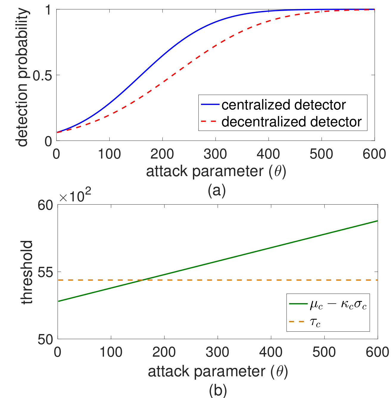 Figure 1
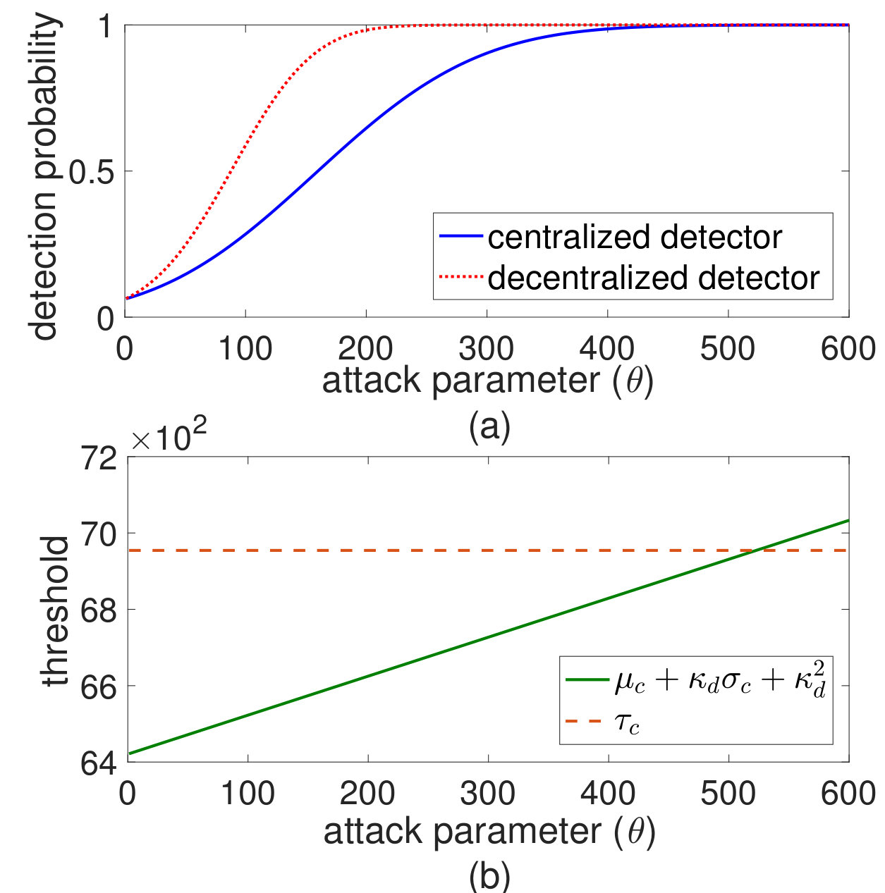 Figure 2
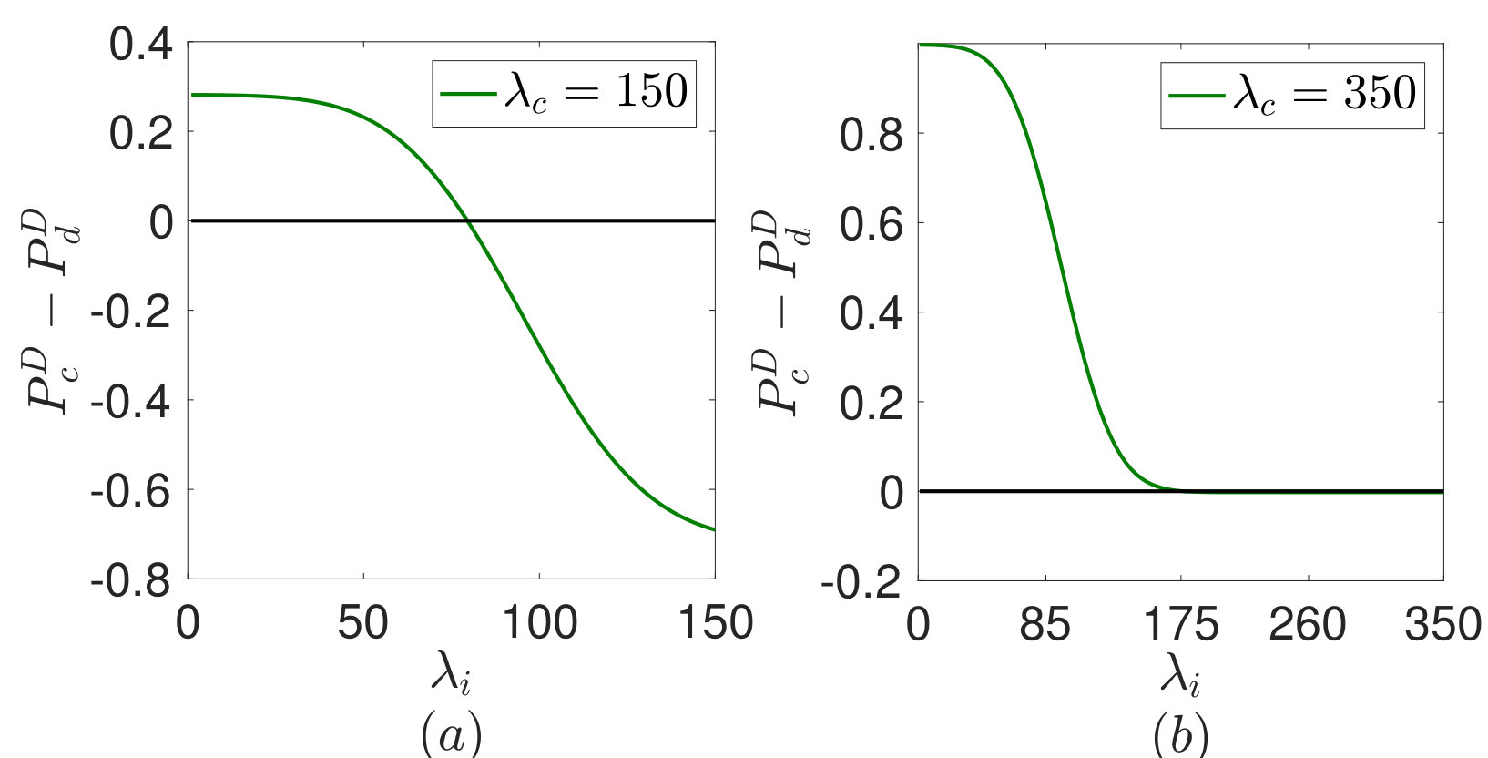 Figure 5
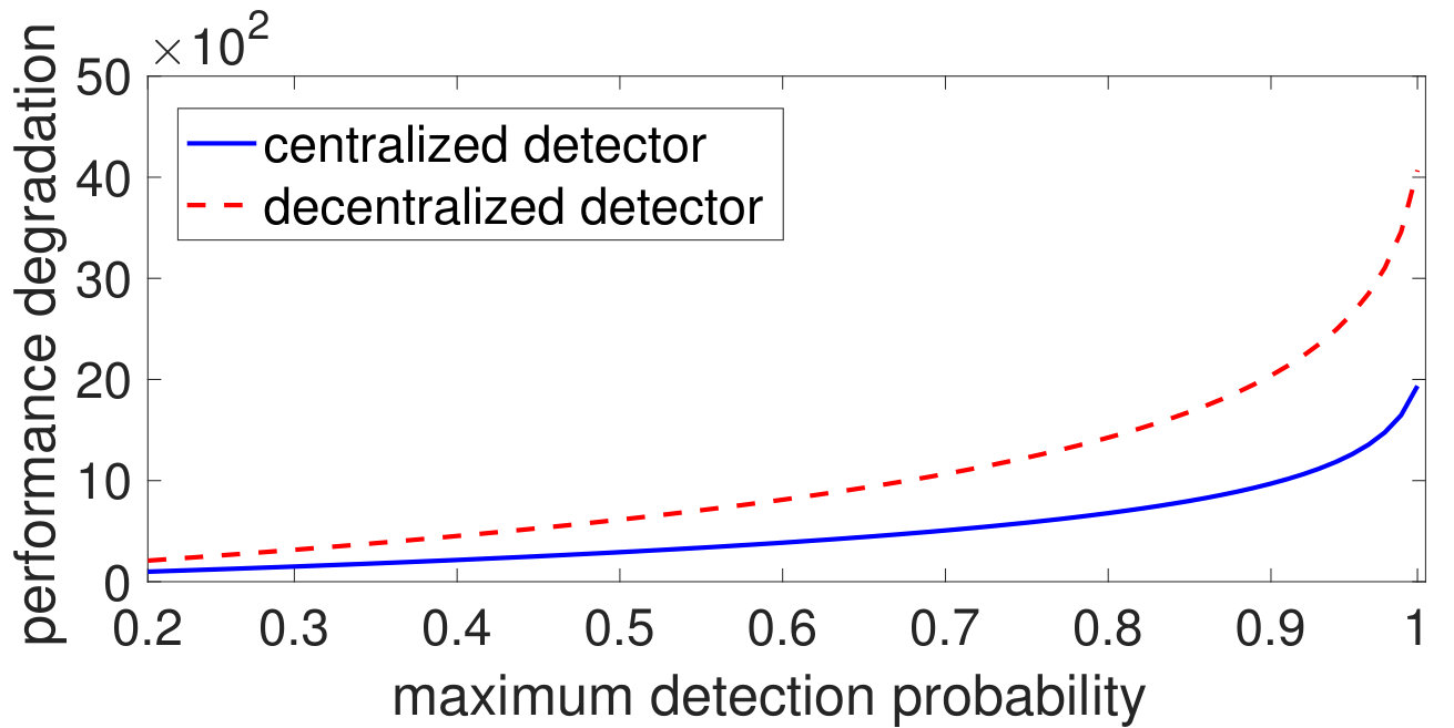 Figure 6
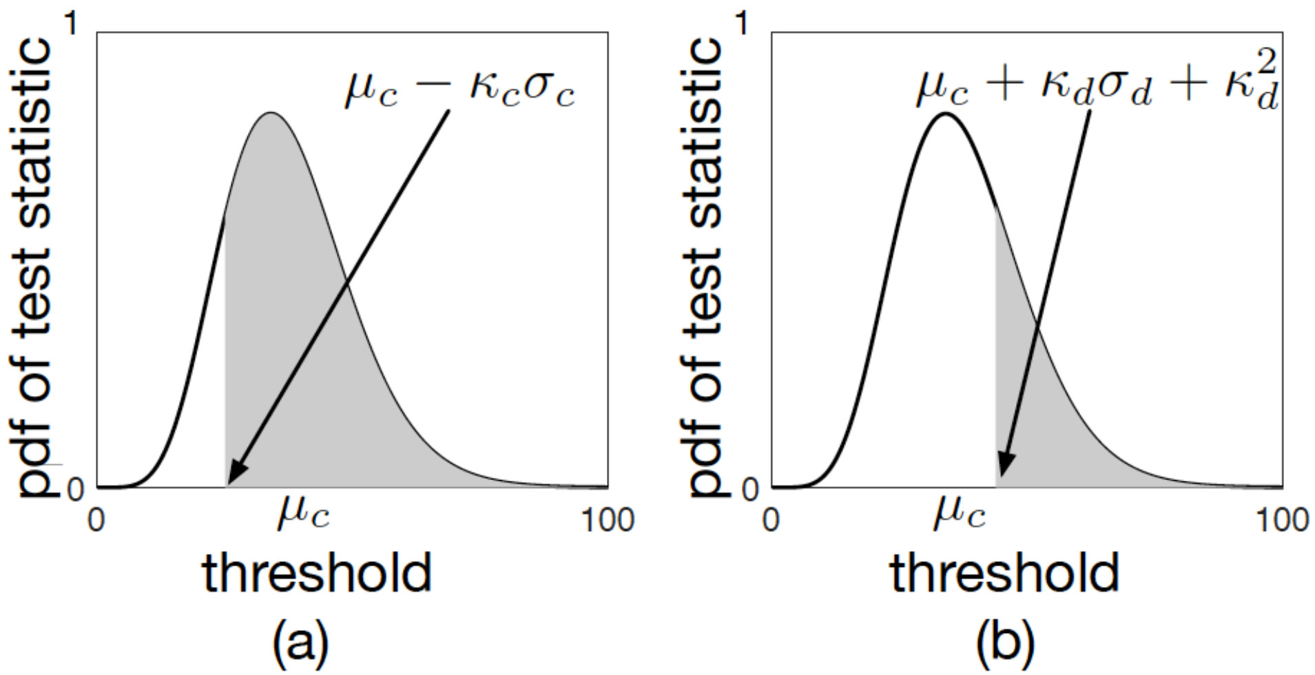 Figure 7
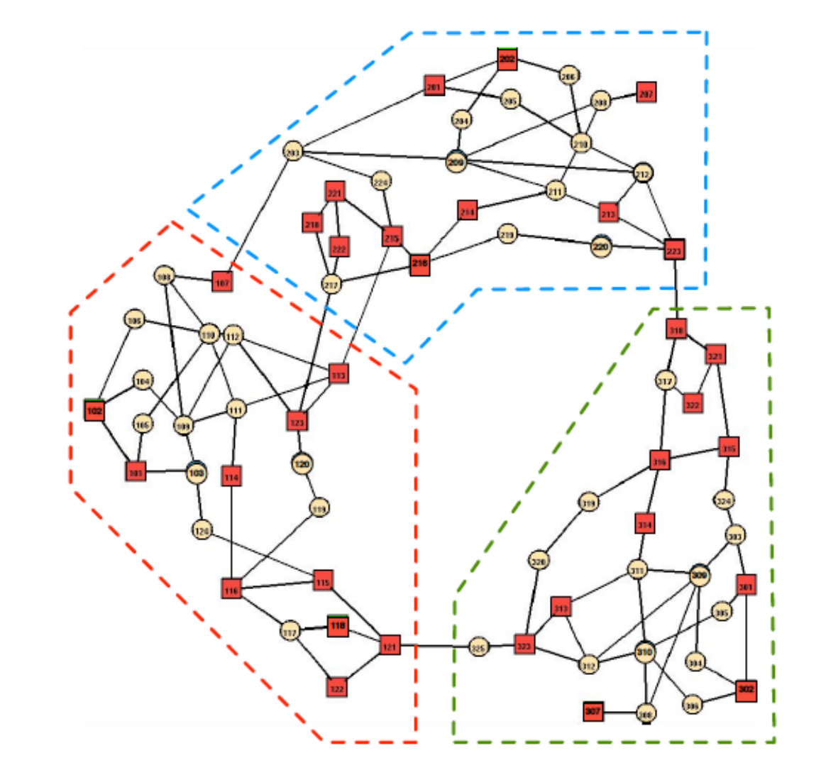 Figure 8
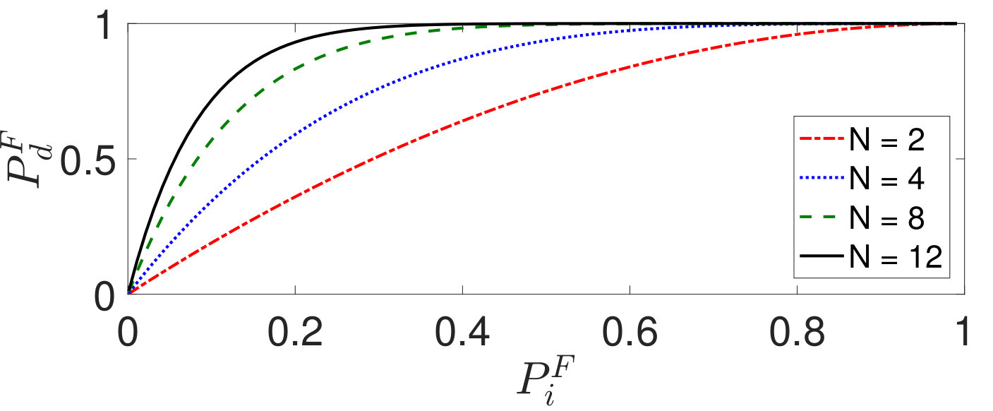 Figure 9
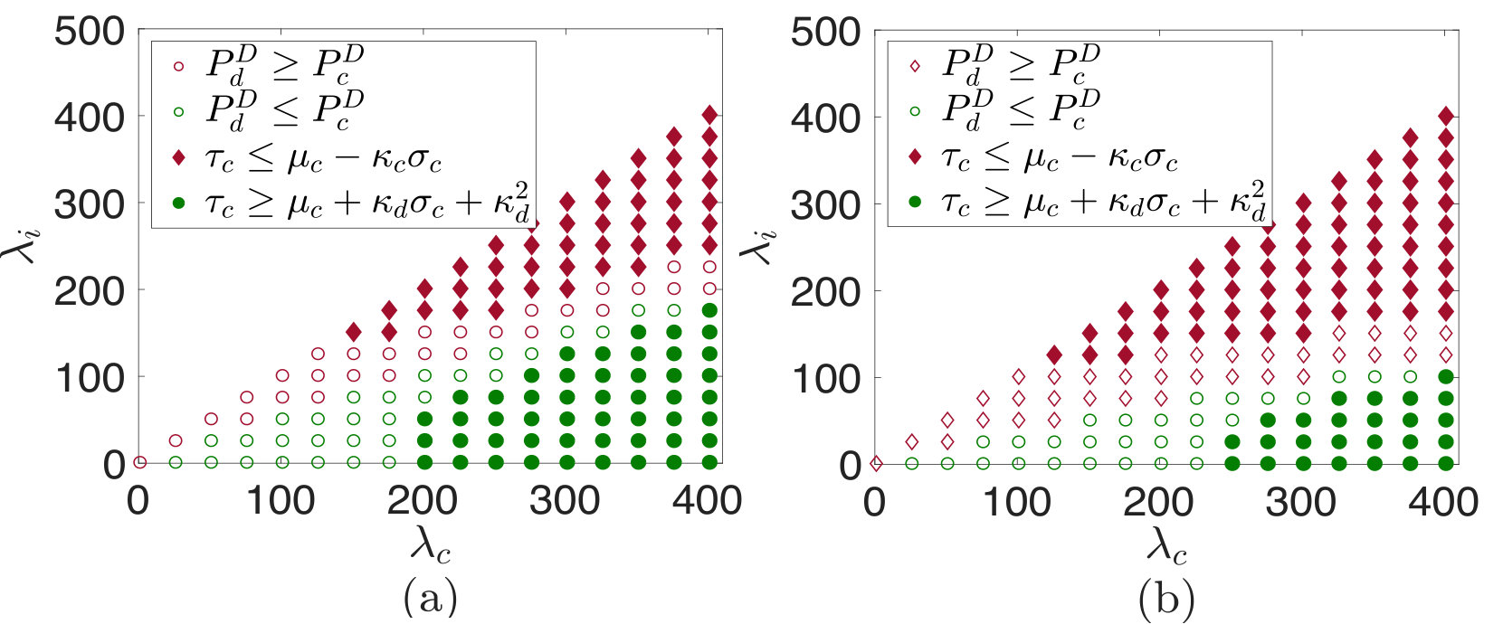 Figure 10
Peer Reviews
No public reviews on file for this paper yet. If you reviewed it on a platform where reviews are public (OpenReview, ICLR, NeurIPS, ICML), you can paste yours below so the community can read it here.
Videos
No videos yet. Explain this paper in a talk, walkthrough, or lecture? Add one.
\setstackEOL
Centralized Versus Decentralized Detection of Attacks in
Stochastic Interconnected Systems
Rajasekhar Anguluri
\IEEEmembershipStudent Member, IEEE
Vaibhav Katewa
\IEEEmembershipMember, IEEE
and Fabio Pasqualetti \IEEEmembershipMember, IEEE This material is based upon work supported by the awards ARO 71603NSYIP, NSF ECCS1405330, and UCOP LFR-18-548175. The authors are with the Department of Mechanical Engineering, University of California, Riverside, {rangu003,vkatewa,fabiopas}@engr.ucr.edu.
Abstract
We consider a security problem for interconnected systems governed by linear, discrete, time-invariant, stochastic dynamics, where the objective is to detect exogenous attacks by processing the measurements at different locations. We consider two classes of detectors, namely centralized and decentralized detectors, which differ primarily in their knowledge of the system model. In particular, a decentralized detector has a model of the dynamics of the isolated subsystems, but is unaware of the interconnection signals that are exchanged among subsystems. Instead, a centralized detector has a model of the entire dynamical system. We characterize the performance of the two detectors and show that, depending on the system and attack parameters, each of the detectors can outperform the other. In particular, it may be possible for the decentralized detector to outperform its centralized counterpart, despite having less information about the system dynamics, and this surprising property is due to the nature of the considered attack detection problem. To complement our results on the detection of attacks, we propose and solve an optimization problem to design attacks that maximally degrade the system performance while maintaining a pre-specified degree of detectability. Finally, we validate our findings via numerical studies on an electric power system.
1 Introduction
Cyber-physical systems are becoming increasingly more complex and interconnected. In fact, different cyber-physical systems typically operate in a connected environment, where the performance of each system is greatly affected by neighboring units. An example is the smart grid, which arises from the interconnection of smaller power systems at different geographical locations, and whose performance depends on other critical infrastructures including the transportation network and the water system. Given the interconnected nature of large cyber-physical systems, and the fact that each subsystem usually has only partial knowledge or measurements of other interconnected units, the security question arises as to whether sophisticated attackers can hide their action to the individual subsystems while inducing system-wide critical perturbations.
In this work we investigate whether, and to what extent, coordination among different subsystems and knowledge of the global system dynamics is necessary to detect attacks in interconnected systems. In fact, while existing approaches for the detection of faults and attacks typically rely on a centralized detector [1, 2, 3], the use of local detectors would not only be computationally convenient, but it would also prevent the subsystems from disclosing private information about their plants. As a counterintuitive result, we will show that local and decentralized detectors can, in some cases, outperform a centralized detector, thus supporting the development of distributed and localized theories and tools for the security of cyber-physical systems.
Related work: Centralized attack detectors have been the subject of extensive research in the last years [4, 5, 6, 7, 8, 9, 10, 11, 12], where the detector has complete knowledge of the system dynamics and all measurements. Furthermore, these studies use techniques from various disciplines including game theory, information theory, fault detection and signal processing, and have a wide variety of applications [2]. Instead, decentralized attack detectors, where each local detector decides on attacks based on partial information and measurements about the system, and local detectors cooperate to improve their detection capabilities, have received only limited and recent attention [13, 14, 15, 16, 17].
Decentralized detection schemes have also been studied for fault detection and isolation (FDI). In such schemes, multiple local detectors make inferences about either the global or local process, and transmit their local decisions to a central entity, which uses appropriate fusion rules to make the global decision[18, 19, 20, 21, 22]. Methods to improve the detection performance by exchanging information among the local detectors have also been proposed [23, 24, 25]. These decentralized algorithms are typically complex [1], their effectiveness in detecting unknown and unmeasurable attacks is difficult to characterize, and their performance is believed to be inferior when compared to their centralized counterparts. To the best of our knowledge, a rigorous comparison of centralized and decentralized attack detection schemes is still lacking, which prevents us from assessing whether, and to what extent, decentralized and distributed schemes should be employed for attack detection and identification.
Main contributions:111In a preliminary version of this paper [26], we used asymptotic approximations to compare the detectors’ performance. Instead, in this paper we provide stronger, tight, and non-asymptotic results without using any approximations. Further, it contains new results on the design of optimal undetectable attacks, and a characterization of the performance degradation induced by such attacks. In addition, an illustration of the results using electrical power grid is also presented. This paper features three main contributions. First, we propose centralized and decentralized schemes to detect unknown and unmeasurable sensor attacks in stochastic interconnected systems. Our detection schemes are based on the statistical decision theoretic framework that falls under the category of simple versus composite hypotheses testing. We characterize the probability of false alarm and the probability of detection for both detectors, as a function of the system and attack parameters. Second, we compare the performance of the centralized and decentralized detectors, and show that each detector can outperform the other for certain system and attack configurations. We discuss that this counterintuitive phenomenon is inherent with the simple versus composite nature of the considered attack detection problem, and provide numerical examples of this behavior. Third, we formulate and solve an optimization problem to design attacks against interconnected systems that maximally affect the system performance as measured by the mean square deviation of the state while remaining undetected by the centralized and decentralized detectors with a pre-selected probability. Finally, we validate our theoretical findings on the IEEE RTS-96 power system model.
Paper organization: The rest of the paper is organized as follows. Section 2 contains our problem formulation. In Section 3, we present our local, decentralized, and centralize detectors, and characterize their performance. Section 4 contains our main results regarding the comparison of the performance of centralized and decentralized detectors. Section 5 contains the design of optimal undetectable attacks. Finally, Section 6 contains our numerical studies, and Section 7 concludes the paper.
Mathematical notation: The following notation will be adopted throughout the paper. Let be arbitrary sets, then and denotes the union and intersection of the sets, respectively. , , and denote the trace, rank, and null space of a matrix, respectively. () denotes that is a positive definite (positive semi definite) matrix. denotes the Kronecker product for matrices. denotes the block diagonal matrix with as diagonal entries. The identity matrix is denoted by (or to denote dimension explicitly). denotes the probability of the event . The mean and covariance of a real or vector valued random variable is denoted by and . Further, for a real valued random variable , we denote the standard deviation as . If follows a Gaussian distribution, we denote it by . Instead, if follows a noncentral chi-squared distribution, we denote it by , where is the degrees of freedom and is the non-centrality parameter. For and , denotes the complementary cumulative distribution function of .
2 Problem setup and preliminary notions
We consider an interconnected system with subsystems, where each subsystem obeys the discrete-time linear dynamics
[TABLE]
with . In the above equation, the vectors and are the state and measurement of the th subsystem, respectively. The process noise and the measurement noise are independent stochastic processes, and is assumed to be independent of , for all . Further, the noise vectors across different subsystems are assumed to be independent at all times. The th subsystem is coupled with the other subsystems through the term , which takes the form
[TABLE]
The input represents the cumulative effect of subsystems on subsystem . Hence, we refer to as to the interconnection matrix, and to as to the interconnection signal, respectively.
We allow for the presence of attacks compromising the dynamics of the subsystems, and model such attacks as exogenous unknown inputs. In particular, the dynamics of the th subsystem under the attack with matrix read as
[TABLE]
where . In vector form, the dynamics of the interconnected system under attack read as
[TABLE]
where , with standing for , , , , , , , and . Moreover, as the components of the vectors and are independent and Gaussian, and , respectively, where and . Further,
[TABLE]
and .
We assume that each subsystem is equipped with a local detector, which uses the local measurements and knowledge of the local dynamics to detect the presence of local attacks. In particular, the th local detector has access to the measurements in (1), knows the matrices , , and , and the statistical properties of the noise vectors and . Yet, the th local detector does not know or measure the interconnection input , and the attack parameters and . Based on this information, the th local detector aims to detect whether . The decisions of the local detectors are then processed by a decentralized detector, which aims to detect the presence of attacks against the whole interconnected system based on the local decisions. Finally, we assume the presence of a centralized detector, which has access to the measurements in (3), and knows the matrix and the statistical properties of the overall noise vectors and . Similarly to the local detectors, the centralized detector does not know or measure the attack parameters and , and aims to detect whether . We postpone a detailed description of our detectors to Section 3. To conclude this section, note that the decentralized and centralized detectors have access to the same measurements. Yet, these detectors differ in their knowledge of the system dynamics, which determines their performance as explained in Section 4.
Remark 1
(Control input and initial state) The system setup in (2) and (3) typically includes a control input. However, assuming that each subsystem knows its control input, it can be omitted without affecting generality. Further, as the detectors do not have information about the initial state, we assume without loss of generality, that the initial state is deterministic and unknown to the detectors.
3 Local, decentralized, and centralized detectors
In this section we formally describe our local, decentralized, and centralized detectors, and characterize their performance as a function of the available measurements and knowledge of the system dynamics. To this aim, let be an arbitrary time horizon and define the vectors
[TABLE]
which contains the measurements available to the th detector, and
[TABLE]
which contains the measurements available to the centralized detector. Both the local and centralized detectors perform the following three operations in order:
Collect measurements as in (4) and (5), respectively; 2. 2.
Process measurements to filter unknown variables; and 3. 3.
Perform statistical hypotheses testing to detect attacks (locally or globally) using the processed measurements.
The decisions of the local detectors are then used by the decentralized detector, which triggers an alarm if any of the local detectors does so. We next characterize how the detectors process their measurements and perform attack detection via statistical hypothesis testing.
3.1 Processing of measurements
The measurements (4) and (5) depend on parameters that are unknown to the detectors, namely, the system initial state and the interconnection signal (although the process and measurement noises are also unknown, the detectors know their statistical properties). Thus, to test for the presence of attacks, the detectors first process the measurement vectors to eliminate their dependency on the unknown parameters. To do so, using equations (1) and (2), define the observability matrix and the attack, interconnection, and noise forced response matrices of the th subsystem as
[TABLE]
[TABLE]
Analogously, for the system model (3) define the matrices , , and , which are constructed as above by replacing , , and with , , and , respectively. The measurements (4) and (5) can be written as follows:
[TABLE]
where . The vectors , , and are the time aggregated signals of , , , and , respectively, and are defined similarly to . Instead, , and is defined similarly to . To eliminate the dependency from the unknown variables, let and be bases of the left null spaces of the matrices and , respectively, and define the processed measurements as
[TABLE]
where the expressions for and follows from (6) and (7). Notice that, in the absence of attacks (), the measurements and depend only on the system noise. Instead, in the presence of attacks, such measurements also depend on the attack vector, which may leave a signature for the detectors.222If , then and the processed measurements do not depend on the attack. Thus, our local detection technique can only be successful against attacks that do not satisfy this condition. We now characterize the statistical properties of and .
Lemma** 3.1**
(Statistical properties of the processed measurements) The processed measurements and satisfy
[TABLE]
where
[TABLE]
A proof of Lemma 3.1 is postponed to the Appendix. From Lemma 3.1, the mean vectors and depend on the attack vector, while the covariance matrices and are independent of the attack. This observation motivates us to develop a detection mechanism based on the mean of the processed measurements, rather the covariance matrices.
3.2 Statistical hypothesis testing framework
In this section we detail our attack detection mechanism, which we assume to be the same for all local and centralized detectors, and we characterize its false alarm and detection probabilities. We start by analyzing the test procedure of the th local detector. Let be the null hypothesis, where and the system is not under attack, and let be the alternative hypothesis, where and the system is under attack. To decide which hypothesis is true, or equivalently whether the mean value of the processed measurements is zero, we resort to the generalized log-likelihood ratio test (GLRT):
[TABLE]
where the threshold is selected based on the desired false alarm probability of the test (11) [27]. For a statistical hypothesis testing problem, the false alarm probability equals the probability of deciding for when is true, while the detection probability equals the probability of deciding for when is true. While the former is used for tuning the threshold, the latter is used for measuring the performance of the test. Formally, the false alarm and detection probabilities of (11) are the probabilities that are conditioned on the hypothesis and , respectively, and are symbolically denoted as
[TABLE]
Similarly, the centralized detector test is defined as
[TABLE]
where is a preselected threshold, and its false alarm and detection probabilities are denoted as and . We next characterize the false alarm and detection probabilities of the detectors with respect to the system and attack parameters.
Lemma** 3.2**
(False alarm and detection probabilities of local and centralized detectors) The false alarm and the detection probabilities of the tests (11) and (12) are, respectively,
[TABLE]
where
[TABLE]
and
[TABLE]
Lemma 3.2, whose proof is postponed to the Appendix, allows us to compute the false alarm and detection probabilities of the detectors using the decision thresholds, the system parameters, and the attack vector. Moreover, for fixed and , the detection thresholds are computed as and , where is the inverse of the complementary Cumulative Distribution Functions (CDF) that is associated with a central chi-squared distribution. The parameters , and , in Lemma 3.2 are referred to as degrees of freedom and non-centrality parameters of the detectors.
Remark 2
(System theoretic interpretation of detection probability parameters) The degrees of freedom and the non-centrality parameters quantify the knowledge of the detectors about the system dynamics and the energy of the attack signal contained in the processed measurements. In particular:
(Degrees of freedom ) The detection probability and the false alarm probability are both increasing functions of the degrees of freedom , because the function in (13) is an increasing function of . Thus, increasing by, for instance, increasing the number of sensors or the horizon , does not necessarily lead to an improvement of the detector performance.
(Non-centrality parameter ) The non-centrality parameter measures the energy of the attack signal contained in the processed measurements. In the literature of communication and signal processing, the non-centrality parameter is often referred to as signal to noise ratio (SNR) **[27]**. For fixed and , the detection probability increases monotonically with , and approaches the false alarm probability as tends to zero.
*(Decision threshold ) For fixed and , the probability of detection and the false alarm probability are monotonically decreasing functions of the detection threshold . This is due to the fact that the complementary CDFs, which define the false alarm and detection probabilities, are decreasing functions of . As we show later, because of the contrasting behaviors of the false alarm and detection probabilities with respect to all individual parameters, the decentralized detector can outperform the centralized detector. *
We now state a result that provides a relation between the degrees of freedom ( and ) and the non-centrality parameters ( and ) of the local and the centralized detectors. This result plays a central role in comparing the performance of these centralized and decentralized detectors.
Lemma** 3.3**
(Degrees of freedom and non-centrality parameters) Let , and , be the degrees of freedom and non-centrality parameters of the th local and centralized detectors, respectively. Then, and for all .
A proof of Lemma 3.3 is postponed to the Appendix. In loose words, given the interpretation of the degrees of freedom and noncentrality parameters in Remark 2, Lemma (3.3) states that a centralized detector has more knowledge about the system dynamics () and its measurements contain a stronger attack signature () than any of the th local detector. Despite these properties, we will show that the decentralized detector can outperform the centralized one.
4 Comparison of centralized and decentralized detection of
attacks
In this section we characterize the detection probabilities of the decentralized and centralized detectors, and we derive sufficient conditions for each detector to outperform the other. Recall that the decentralized detector triggers an alarm if any of the local detectors detects an alarm. In other words,
[TABLE]
where and denote the false alarm and detection probabilities of the decentralized detector, respectively.
Lemma** 4.1**
(Performance of the decentralized detector) The false alarm and detection probabilities in (16) satisfy
[TABLE]
A proof of Lemma 4.1 is postponed to the Appendix. As shown in Fig. 1, for the case when , for all , increases with increase in and . To allow for a fair comparison between the decentralized and centralized detectors, we assume that . Consequently, for a fixed false alarm probability , the probabilities satisfy
[TABLE]
We now derive a sufficient condition for the centralized detector to outperform the decentralized detector.
Theorem** 4.2**
(Sufficient condition for ) Let , and assume that the following condition is satisfied:
[TABLE]
where . Then, .
A proof of Theorem 4.2 is postponed to the Appendix. We next derive a sufficient condition for the decentralized detector to outperform the centralized detector.
Theorem** 4.3**
(Sufficient condition for ) Let , and assume that the following condition is satisfied:
[TABLE]
where . Then .
A proof of Theorem 4.2 is postponed to the Appendix. Theorems 4.2 and 4.3 provide sufficient conditions on the detectors and attack parameters that result in one detector outperforming the other. In particular, from (18) and (19) we note that, depending on decision threshold , a centralized detector may or may not outperform a decentralized detector. This is intuitive as the function, which quantifies the detection probability, is a decreasing function of the detection threshold (see Remark 2). To clarify the effect of attack and detection parameters on the performance trade-offs of the detectors, we now express (18) and (19) using the mean and standard deviation of the test statistic in (12). Let
[TABLE]
where the expectation and standard deviation (SD) of follows from the fact that under , (see proof of Lemma 3.2). Hence, (18) and (19) can be rewritten, respectively, as
[TABLE]
From (20a) and (20b) we note that a centralized detector outperforms the decentralized one if is standard deviations smaller than the mean . Instead, a decentralized detector outperforms the centralized detector if is at least standard deviations larger than the mean . See Fig. 2 for a graphical illustration of this interpretation.
Theorems 4.2 and 4.3 are illustrated in Fig. 3 as a function of the non-centrality parameters. It can be observed that (i) each of the detectors can outperform the other depending on the values of the noncentrality parameter values, (ii) the provided bounds qualitatively capture the actual performance of the centralized and decentralized detectors as the non-centrality parameters increase, and (iii) the provided bounds are rather tight over a large range of non-centrality parameters. In Fig. 4 we show that the difference of the detection probabilities of the centralized and decentralized detectors can be large, especially when the non-centrality parameters are small and satisfy , as evident in panel (a) of Fig. 4 .
5 Design of optimal attacks
In this section we consider the problem of designing attacks that deteriorate the performance of the interconnected system (1) while remaining undetected from the centralized and decentralized detectors. We measure the degradation induced by an attack with the expected value of the deviation of the state trajectory from the origin. We assume that the attack is a deterministic signal, and thus independent of the noise affecting the system dynamics and measurements. In particular, for a fixed value of the probability and a threshold , we consider the optimization problem
[TABLE]
where is the deterministic attack input over time horizon (see (7)). Notice that, because the attack is deterministic, the objective function in (P.1) can be simplified by bringing the expectation inside the summation, and replacing the state equation constraint with the mean state response. Further, because the system parameters and are fixed, and are also fixed, which ensures that only depends on noncentrality parameter. This observation along with the fact that is increasing function in noncentrality parameter (see Remark 2) allows us to express the detection constraint in terms of . Specifically, the optimization problem (P.1) can be rewritten as
[TABLE]
where we have used that is independent of the attack , and
[TABLE]
with . Further, we have , where denotes the inverse of for fixed and , and , with as in (15). It should be noticed that the attack constraint in (P.2) essentially limits the (weighted) energy of the attack signal. We next characterize the solution to the optimization problem (P.2).
Theorem** 5.1**
(Optimal attack vectors) Let be any solution of (P.2). Then, there exist a such that the pair solves the following optimality equations:
[TABLE]
where
[TABLE]
A proof of Theorem 5.1 is postponed to the Appendix. Theorem 5.1 not only guarantees the existence of optimal attacks, but it also provides us with necessary conditions to verify if an attack is (locally) optimal. When the system initial state is zero, we can also quantify the performance degradation induced by an optimal attack. Let and denote a largest generalized eigenvalue of a matrix pair and one of its associated generalized eigenvectors [28].
Lemma** 5.2**
(System degradation with zero initial state) Let . Then, the optimal solution to (P.2) is
[TABLE]
and its associated optimal cost is
[TABLE]
where .
A proof of Lemma 5.2 is postponed to the Appendix. From (24), notice that the system degradation caused by an optimal attack depends on the detector’s tolerance, as measured by , and the system dynamics, as measured by . See Remark 4 for the influence of processed measurement’s noise uncertainty on the system degradation due to optimal attacks.
Remark 3
(Optimal attack vector against decentralized detector) To characterize the performance degradation of the system analytically, we consider a relaxed form of detection constraint. Specifically, we design optimal attacks subjected to instead of , where is an upper bound on (see Lemma 1.3). The design of optimal attacks that are undetectable from the decentralized detector can be formulated in the following way:
[TABLE]
where the summation in the detectability constraint follows from Lemma 1.3 and the fact that becomes equivalent to , where , , and . Let be a permutation matrix such that , and let and . For any solution of (P.2), there exist such that the pair solves the following optimality equations:
[TABLE]
Further, if , then the largest degradation is .
Remark 4
(Maximum degradation of the system performance with respect to system noise) To see the role of noise level, in the processed measurements, on the system degradation, we consider the following covariance matrices: and , for . Then, from (24) we have
[TABLE]
where . From (25) we note that the system degradation increases with the increase in the noise level, i.e., .
6 Numerical comparison of centralized and decentralized
detectors
In this section, we demonstrate our theoretical findings on the IEEE RTS-96 power network model [29], which we partition into three subregions as shown in Fig. 5. We followed the approach in [30] to obtain a linear time-invariant model of the power network, and then discretized it using a sampling time of seconds. For a false alarm probability , we consider the family of attacks , where is the vector of all ones and . It can be shown that the noncentrality parameters satisfy and , and moreover, the choice of vector is arbitrary and it does not affecting the following results.
(Illustration of Theorem 4.2) For the measurement horizon of seconds, the values of and are and , respectively. Fig. 6 show that the detection probabilities of the centralized and decentralized detectors increase monotonically with the attack parameter . As predicted by the sufficient condition (20a) and shown in Fig. 6, the centralized detector is guaranteed to outperform the decentralized detector when . This figure also shows that our condition is conservative, because for all values of as shown in Fig. 6.
(Illustration of Theorem 4.3) Contrary to the previous example, by letting seconds, we obtain and . For these choice of parameters, the decentralized detector is guaranteed to outperform the centralized detector when . This behavior is predicted by our sufficient condition (20b), and it is illustrated in Fig. 7. As in the previous example, the estimation provided by our condition (20b) is conservative, as illustrated in Fig. 7.
(Illustration of Lemma 5.2) In Fig. 8 we compare the performance degradation induced by the optimal attacks designed according to the optimization problems (P.2) and (P.3) with zero initial conditions. In particular, we plot the optimal costs and against the tolerance levels and , respectively. As expected, the performance degradation is proportional to the tolerance levels and, for the considered setup, it is larger in the case of the decentralized detector.
7 Conclusion
In this work we compare the performance of centralized and decentralized schemes for the detection of attacks in stochastic interconnected systems. In addition to quantifying the performance of each detection scheme, we prove the counterintuitive result that the decentralized scheme can, at times, outperform its centralized counterpart, and that this behavior results due to the simple versus composite nature of the attack detection problem. We illustrate our findings through academic examples and a case study based on the IEEE RTS-96 power system. Several questions remain of interest for future investigation, including the characterization of optimal detection schemes, an analytical comparison of the degradation induced by undetectable attacks as a function of the detection scheme, and the analysis of iterative detection strategies.
APPENDIX
Proof of Lemma 3.1:
Since the attack vectors and are deterministic, and , , , and are zero mean random vectors, from the linearity of the expectation operator it follows from (8) that
[TABLE]
Further, from the properties of , we have the following:
[TABLE]
where (a) follows because the measurement and process noises are independent of each other. Instead, (b) is due to the fact that the noise vectors are independent and identically distributed. Similar analysis also results in the expression of , and hence the details are omitted. Finally, by invoking the fact that linear transformations preserve Gaussianity, the distribution of and is Gaussian as well. \QED
Proof of Lemma 3.2:
From the statistics and distributional form of and (see (9)), and threshold tests defined in (11) and (12), it follows from [31, Theorem 3.3.3] that, under
null hypothesis : and , where and are defined in (14). 2. 2.
alternative hypothesis : and , where and .
By substituting and (see Lemma 3.1) and rearranging the terms, we get the expressions of and in (14). Finally, from the aforementioned distributional forms of and , it now follows that the false alarm and the detection probabilities of the tests (11) and (12) are the right tail probabilities (represented by function) of the central and noncentral chi-squared distributions, respectively. Hence, the expressions in (13) follow. \QED
Proof of Lemma 3.3:
Without loss of generality let . Thus, it suffices to show that a) and b) .
Case (a): For brevity, define
[TABLE]
and note that and . From Lemma 3.1, Lemma 3.2, and (26), we have
[TABLE]
Similarly, . Since, and are a basis vectors of the null spaces and (see (37)) respectively, it follows from Proposition A.1 that .
Case (b): As the proof for this result is rather long and tedious, we break it down in to multiple steps:
- •
Step 1: Express and using the statistics of a permuted version of .
- •
Step 2: Obtain lower bound on , which depends on the statistics of the measurements pertaining to Subsystem 1.
- •
Step 3: Show that is less than bound in Step .
Step 1 (alternative form of and ):
Notice that and in (14) can be expressed as and , respectively, where , , , and are defined in Lemma 3.1. For convenience, we express and in an alternative way. Let and consider the th sensor measurements of (3)
[TABLE]
Also, define and . Now, from (27) and state equation in (3), can be expanded as
[TABLE]
where the matrices , , and are similar to the matrices defined in Section II-A. By substituting the above decomposition of in we have
[TABLE]
Moreover, from the distributional assumptions on and , it readily follows that (similarly to the proof of Lemma 3.1),
[TABLE]
where , and and are defined same as in Lemma 3.1.
Now, consider the measurement equation in (1) and note that . Thus, , for all and . From this observation it follows that , where is a selection matrix. Let and note that . Further from Proposition A.1 we have . With these facts in place, from Lemma 3.1 we now have
[TABLE]
Similarly, since is just a rearrangement of (see (5)), there exists a permutation matrix such that , and, ultimately . Thus,
[TABLE]
Let . From (29) and (30) we have
[TABLE]
Step 2 (lower bound on ):
Since, , it follows that is the basis of the null space . Further, the row vectors of and are linearly independent, whenever . Using these facts we can define such that , where . Let and note that
[TABLE]
Let . Since , it follows that both the matrices and are invertible. Hence, from Schur’s complement, there exists a matrix such that
[TABLE]
Similarly, consider the following partition of :
[TABLE]
where and , and let . Invoking Schur’s complement, we have the following:
[TABLE]
where . Substituting(32) and (33) in (31), we have
[TABLE]
Instead, in (31) can be shown as
[TABLE]
where we used the fact that .
Step 3 ():
For to hold true, it suffices to show the following:
[TABLE]
By invoking Proposition A.1, we note that there exists a full row rank matrix , such that . Since is a full column rank matrix, we can define an invertible matrix , where forms a basis for null space of , such that the following holds
[TABLE]
By invoking Schur’s complement, it follows that
[TABLE]
where . Hence,
[TABLE]
By substituting in the above expression, and rearranging the terms we have
[TABLE]
The required inequality follows by substituting and , and recalling the fact that the sum of two positive semi definite matrices is greater than or equal to either of the matrices. \QED
Proof of Lemma 4.1:
Let be an event that the th local detector decides when the true hypothesis is . Then, . Let be the complement of . Then, from (16) it follows that
[TABLE]
where for the we used the fact that the events are mutually independent for all . To see this fact, notice that the event is defined on (see (8)). Further, depends only on the deterministic attack signal and the noise vectors and , but not on the interconnection signal (see (6)). Now, by invoking the fact that noises variables across different subsystems are independent, it also follows that the events are also mutually independent. Similar procedure will lead to the analogous expression for and hence, the details are omitted. \QED
Proof of Theorem 4.2:
Let and , and assume that (18) holds true. Then, from the monotonicity property of the CDF associated with the test statistic , which follows , we have the following inequality
[TABLE]
From the inequality (41b), it now follows that
[TABLE]
where for the last inequality we used the fact that for all . By using the above inequality and Lemma 3.2, under hypothesis , we have
[TABLE]
Proof of Theorem 4.3
Let and , and assume that (19) holds true. Then, from the monotonicity property of the CDF associated with the test statistic , which follows , we have the following inequality
[TABLE]
From the inequality (41a), it now follows that
[TABLE]
The result follows by substituting in the above inequality. \QED
Proof of Theorem 5.1
By recursively expanding the equality constraint of the optimization problem (P.2) we have
[TABLE]
By using the above identity, (P.2) can also be expressed as
[TABLE]
From the first-order necessary conditions [32] we now have
[TABLE]
where the gradient is with respect to .
Case (i): Suppose . Then should hold true to ensure the complementarity slackness condition (36b). Using these observations in the KKT conditions we now have . Further, since, is a convex function of , by evaluating the second derivative of at , it can be easily seen that the obtained results in minimum value of (P.2) rather than the maximum.Thus, for any of (P.2), the condition cannot hold true.
Case (ii): Suppose . Then the KKT conditions can be simplified to the following:
[TABLE]
The result now follows by evaluating the derivative on the left hand side of the first equality. \QED
Proof of Lemma 5.2
By substituting in (21a), we note that any optimal attack is of the form , where is the generalized eigenvector of the pair [28], and the scalar is obtained from (21b). Let be the optimal cost associated with an attack of the form . Then,
[TABLE]
where the first equality follows from the fact that the objective function in (P.2) can be expressed as , and the second equality follows from (21a). Since is a generalized eigenvector of the pair , it follows that is the eigenvalue corresponding to and hence, is maximized when is maximum, which is obtained for . The result follows since, , for . \QED
Proposition A.1
Let be the observability and impulse response matrices defined in (6). Define
[TABLE]
where and . Then, , for all .
Proof 1.2**.**
Without loss of generality, let . By definition, the set inclusion is trivial. For the other inclusion, consider the system defined in (3) without the attack and noise, i.e., . Let , where and are the state and the interconnection signal of Subsystem . Also, let
[TABLE]
Notice that, can be decomposed as
[TABLE]
By letting and recursively expanding using (39), we have
[TABLE]
where the second, third, and fourth equalities follows from (38), system , and (39), respectively. By recalling that , it follows from (1.2) that
[TABLE]
Let be any vector such that . Then, also satisfies . Thus, .
Lemma 1.3**.**
(Upper bound on ) Let and be defined as in (14), and be defined as in (11). Let , , and . Then,
[TABLE]
where .
Proof 1.4**.**
Consider the following events:
[TABLE]
where the event is associated with the th local detector’s threshold test. From the definition of the above events, it is easy to note that . By the monotonicity of the probability measures, it follows that
[TABLE]
From the reproducibility property of the noncentral chi-squared distribution [33], it now follows that equals in distribution and hence, .
Lemma 1.5**.**
(Exponential bounds on the tails of ) Let , , . For all ,
[TABLE]
Proof 1.6**.**
See [34].
The reference list from the paper itself. Each links out to its DOI / PubMed record.
- 1[1] F. Pasqualetti, F. D rfler, and F. Bullo, “Attack detection and identification in cyber-physical systems,” IEEE Transactions on Automatic Control , vol. 58, no. 11, pp. 2715–2729, Nov 2013.
- 2[2] Y. Lun, A. D’Innocenzo, I. Malavolta, M. Domenica, and D. Benedetto, “Cyber-physical systems security: a systematic mapping study,” arxiv , 2016, available at https://arxiv.org/pdf/1605.09641.pdf.
- 3[3] J. Chen and R. Patton, Robust Model-Based Fault Diagnosis for Dynamic Systems . Springer-Verlag New York, 1999.
- 4[4] Y. Yuan, Q. Zhu, F. Sun, Q. Wang, and T. Basar, “Resilient control of cyber-physical systems against denial-of-service attacks,” in 2013 6th International Symposium on Resilient Control Systems (ISRCS) , Aug 2013, pp. 54–59.
- 5[5] H. Fawzi, P. Tabuada, and S. Diggavi, “Secure estimation and control for cyber-physical systems under adversarial attacks,” IEEE Transactions on Automatic Control , vol. 59, no. 6, pp. 1454–1467, 2014.
- 6[6] S. Sridhar and M. Govindarasu, “Model-based attack detection and mitigation for automatic generation control,” IEEE Transactions on Smart Grid , vol. 5, no. 2, pp. 580–591, March 2014.
- 7[7] L. Liu, M. Esmalifalak, Q. Ding, V. A. Emesih, and Z. Han, “Detecting false data injection attacks on power grid by sparse optimization,” IEEE Transactions on Smart Grid , vol. 5, no. 2, pp. 612–621, March 2014.
- 8[8] H. Zhang, P. Cheng, L. Shi, and J. Chen, “Optimal denial-of-service attack scheduling with energy constraint,” IEEE Transactions on Automatic Control , vol. 60, no. 11, pp. 3023–3028, Nov 2015.