The exact geostrophic streamfunction for neutral surfaces
Geoffrey J. Stanley

TL;DR
This paper derives the exact geostrophic streamfunction for neutral surfaces using a path integral approach, introduces a practical approximation called the topobaric geostrophic streamfunction, and demonstrates its superior accuracy in estimating oceanic geostrophic velocities.
Contribution
The paper provides the first explicit form of the exact geostrophic streamfunction for neutral surfaces and introduces the topobaric approximation for practical use in oceanography.
Findings
Topobaric geostrophic streamfunction reduces velocity estimation error by an order of magnitude.
The exact streamfunction involves a path integral over a neutral trajectory and is multivalued due to surface holes.
The orthobaric Montgomery potential offers a computationally efficient approximation with improved accuracy.
Abstract
McDougall (1989) proved that neutral surfaces possess an exact geostrophic streamfunction, but its form has remained unknown. The exact geostrophic streamfunction for neutral surfaces is derived here. It involves a path integral of the specific volume along a neutral trajectory. On a neutral surface, the specific volume is a multivalued function of the pressure on the surface, . By decomposing the neutral surface into regions where the specific volume is a single-valued function of , the path integral is simply a sum of integrals of these single-valued functions. The regions are determined by the Reeb graph of , and the neutral trajectory is encoded by a walk on this graph. Islands, and other holes in the neutral surface, can create cycles in the Reeb graph, causing the exact geostrophic streamfunction on a neutral surface to…
Click any figure to enlarge with its caption.
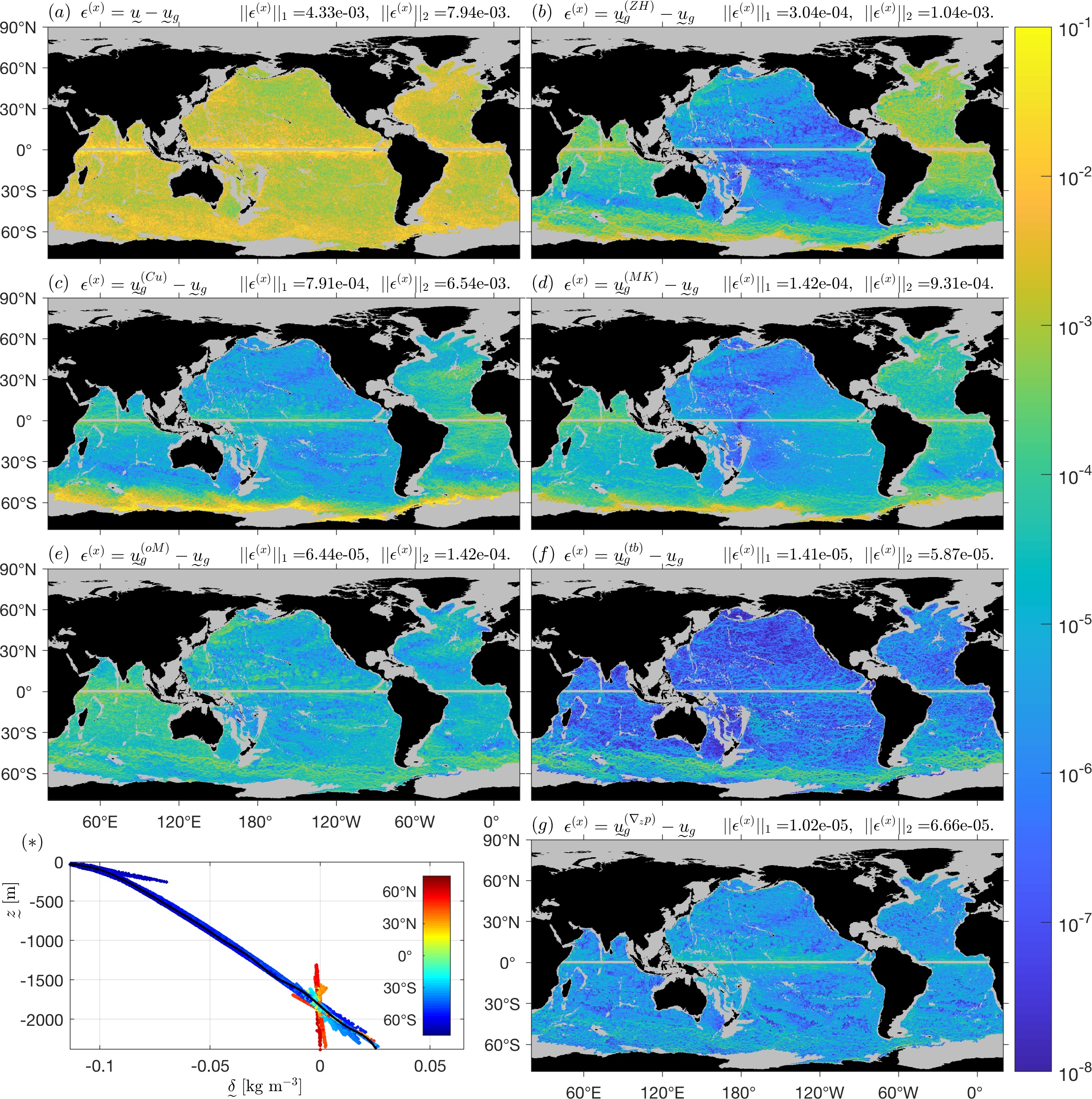 Figure 1
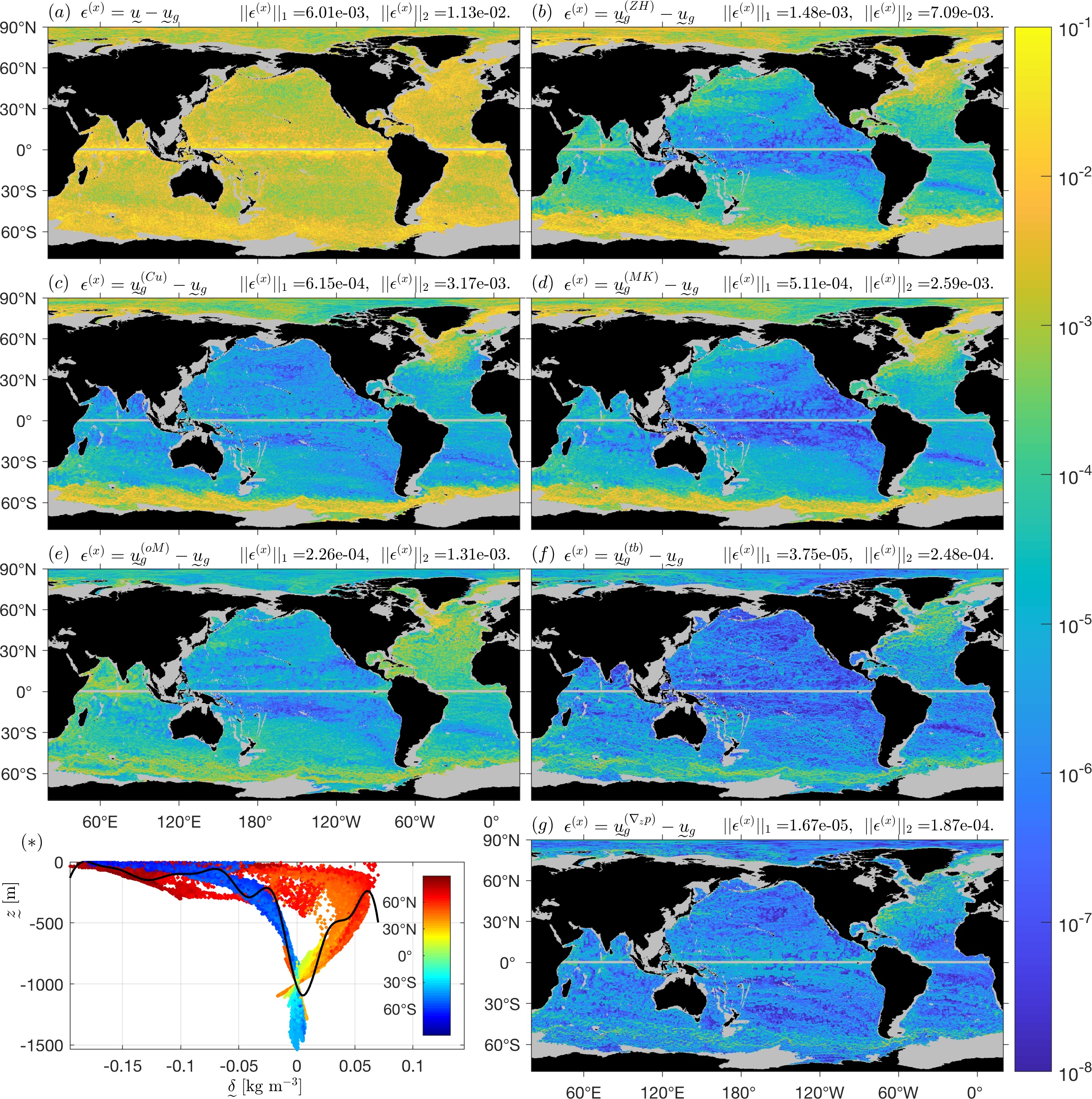 Figure 2
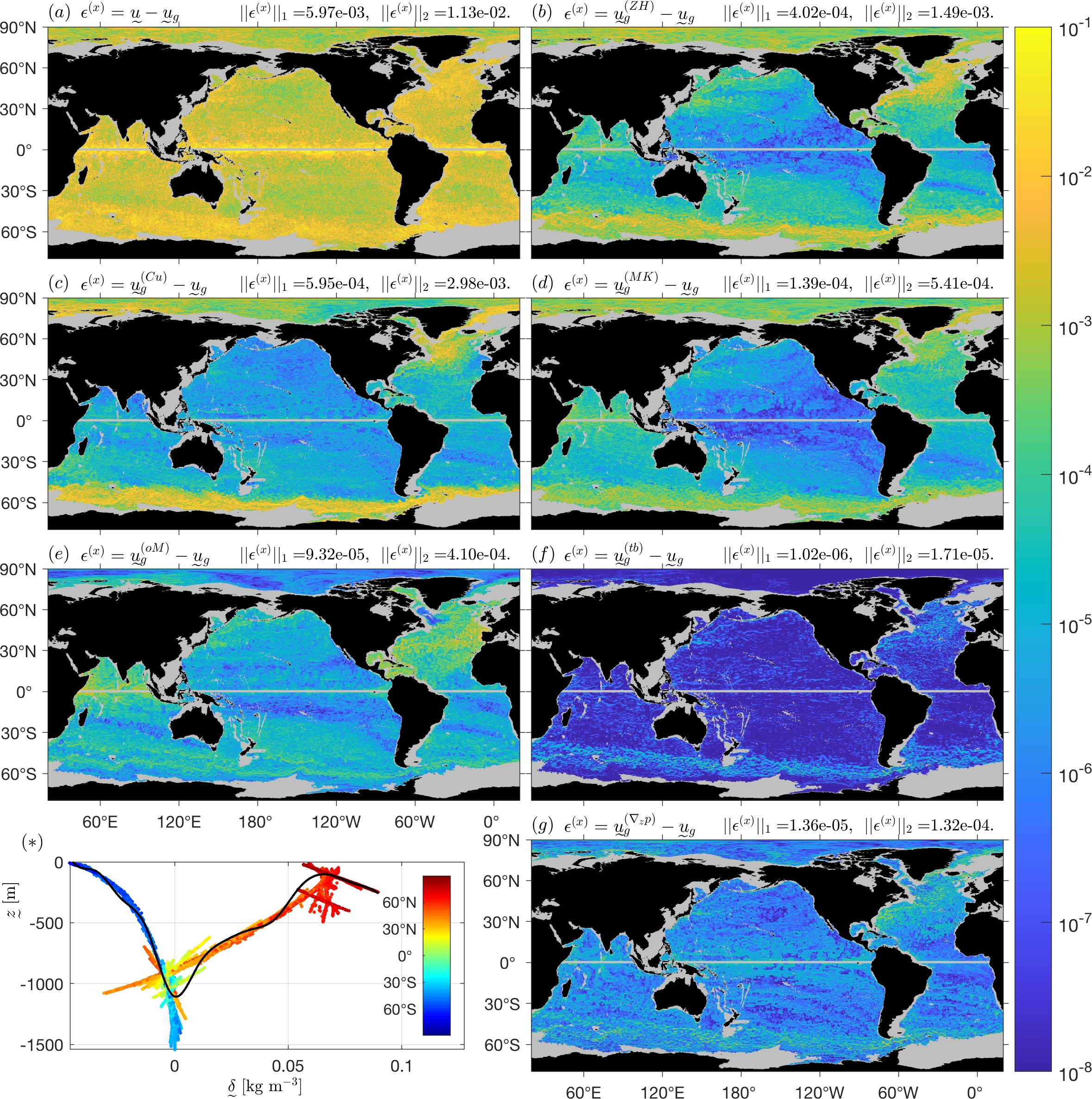 Figure 3
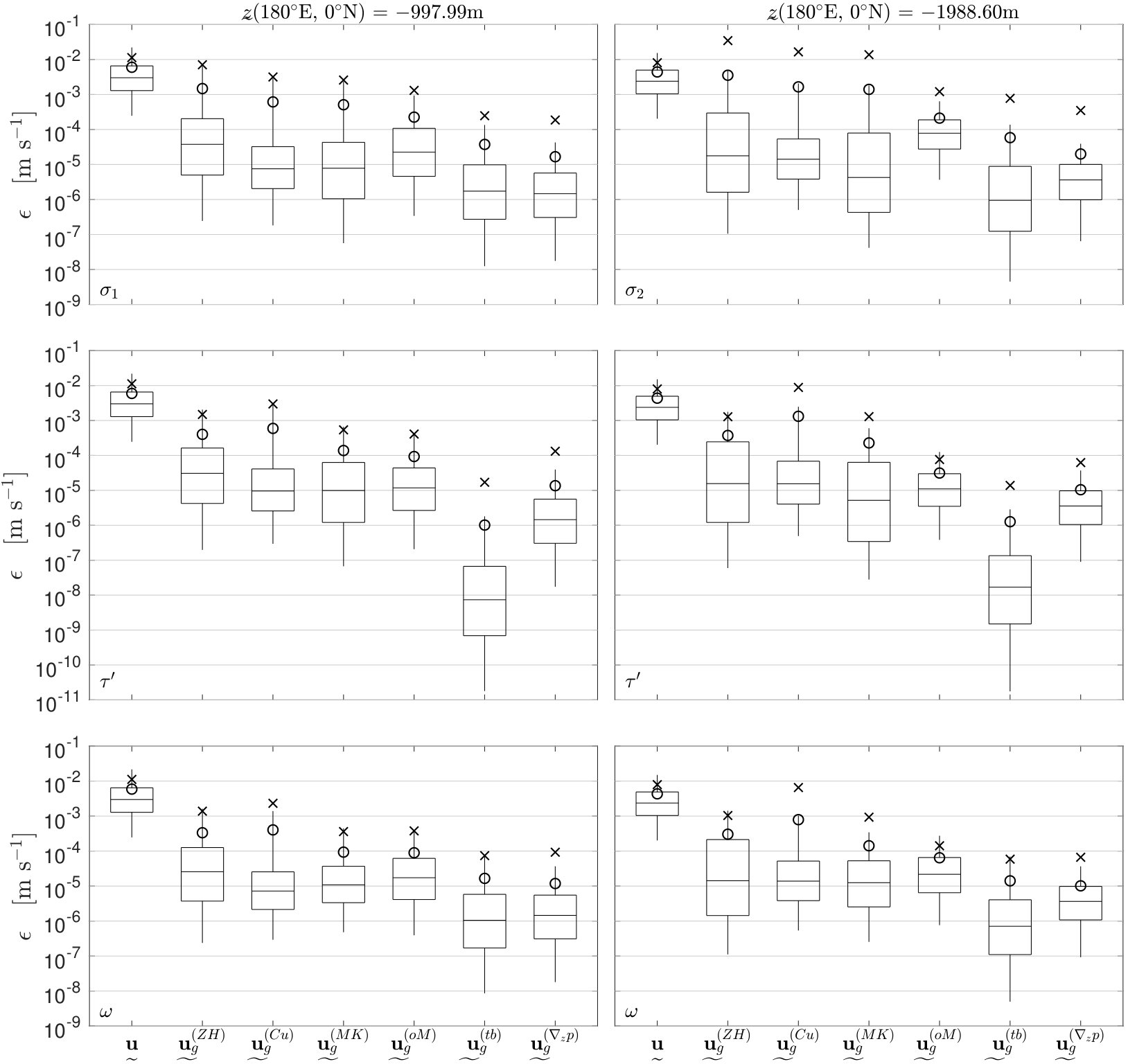 Figure 4
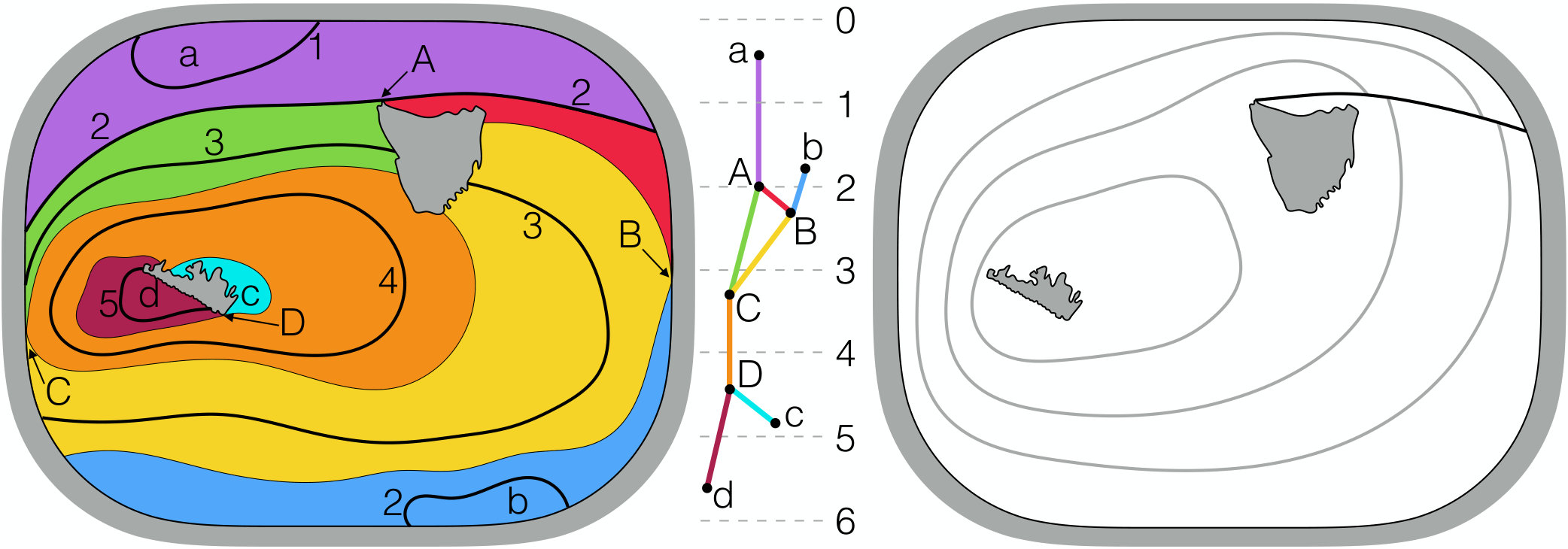 Figure 5
| (a) | ||||||
|---|---|---|---|---|---|---|
| 6.0e-03 | 6.0e-03 | 5.9e-03 | 4.4e-03 | 4.4e-03 | 4.3e-03 | |
| 1.5e-03 | 4.0e-04 | 3.3e-04 | 3.6e-03 | 3.7e-04 | 3.0e-04 | |
| 6.2e-04 | 6.0e-04 | 4.0e-04 | 1.7e-03 | 1.3e-03 | 7.9e-04 | |
| 5.1e-04 | 1.4e-04 | 9.3e-05 | 1.4e-03 | 2.3e-04 | 1.4e-04 | |
| 2.3e-04 | 9.3e-05 | 8.9e-05 | 2.1e-04 | 3.1e-05 | 6.4e-05 | |
| 3.8e-05 | 1.0e-06 | 1.7e-05 | 5.9e-05 | 1.3e-06 | 1.4e-05 | |
| 1.7e-05 | 1.4e-05 | 1.2e-05 | 2.0e-05 | 1.0e-05 | 1.0e-05 | |
| 6.90 | 3.30 | 2.50 | 7.91 | 5.05 | 4.25 | |
| 3.41 | 3.39 | 2.04 | 4.31 | 4.84 | 3.21 | |
| 3.07 | 1.32 | 0.71 | 4.24 | 2.34 | 1.40 | |
| 2.00 | 1.08 | 1.09 | 3.11 | 0.48 | 1.02 | |
| 0.28 | 0.00 | 0.14 | 0.47 | 0.01 | 0.15 | |
| 0.12 | 0.11 | 0.10 | 0.19 | 0.15 | 0.15 | |
Peer Reviews
No public reviews on file for this paper yet. If you reviewed it on a platform where reviews are public (OpenReview, ICLR, NeurIPS, ICML), you can paste yours below so the community can read it here.
Videos
No videos yet. Explain this paper in a talk, walkthrough, or lecture? Add one.
The exact geostrophic streamfunction for neutral surfaces
Geoffrey J. Stanley111Current address: School of Mathematics and Statistics, University of New South Wales, Sydney, NSW 2052, Australia.
© 2019. This manuscript version is made available under the CC-BY-NC-ND 4.0 license http://creativecommons.org/licenses/by-nc-nd/4.0/
Department of Physics, University of Oxford, Oxford, OX1 3PU, United Kingdom
Abstract
McDougall (1989) proved that neutral surfaces possess an exact geostrophic streamfunction, but its form has remained unknown. The exact geostrophic streamfunction for neutral surfaces is derived here. It involves a path integral of the specific volume along a neutral trajectory. On a neutral surface, the specific volume is a multivalued function of the pressure on the surface, . By decomposing the neutral surface into regions where the specific volume is a single-valued function of , the path integral is simply a sum of integrals of these single-valued functions. The regions are determined by the Reeb graph of , and the neutral trajectory is encoded by a walk on this graph. Islands, and other holes in the neutral surface, can create cycles in the Reeb graph, causing the exact geostrophic streamfunction on a neutral surface to be multivalued. Moreover, neutral surfaces are ill-defined in the real ocean. Hence, the topobaric geostrophic streamfunction is presented: a single-valued approximation of the exact geostrophic streamfunction for neutral surfaces, for use on any well-defined, approximately neutral surface. Numerical tests on several approximately neutral surfaces reveal that the topobaric geostrophic streamfunction estimates the geostrophic velocity with an error that is about an order of magnitude smaller than that for any previously known geostrophic streamfunction. Also, the Montgomery potential is generalized, leading to an alternate form of the exact geostrophic streamfunction for neutral surfaces. This form is used to construct the orthobaric Montgomery potential, an easily computable geostrophic streamfunction that estimates the geostrophic velocity more accurately than any previously known geostrophic streamfunction, but less so than the topobaric geostrophic streamfunction.
keywords:
Neutral surface, Geostrophic streamfunction, Multivalued function, Topology, Reeb graph,
††journal: Ocean Modelling
1 Introduction
Outside the mixed layer and bottom boundary layer and on scales larger than about , the structure of oceanic flow is predominantly two-dimensional, largely confined to isosurfaces of a quasi-conservative density. This enabled Reid and Lynn [1971], for example, to draw conclusions about how the deep tropical oceans are connected to the shallow polar oceans. This method of analysis is even more powerful if, rather than just knowing the flow is within such a surface, we can describe the flow within that surface, for example by means of a geostrophic streamfunction (GSF).
A GSF is the potential, in a specified surface, for the acceleration by the horizontal pressure gradient. (Hence, this quantity is sometimes called an “acceleration potential”; nomenclature is discussed at the end of this section.) A GSF is not, technically, a streamfunction of the geostrophic velocity: none exists, because meridional variation of the Coriolis parameter implies the geostrophic velocity is divergent. Still, the geostrophic velocity (a 2D vector field) is exactly determined by the GSF (a scalar field) and the known Coriolis parameter. Moreover, the geostrophic velocity is everywhere (except the equator) tangent to contours of the GSF, which are therefore streamlines of the geostrophic velocity.
GSFs possess many theoretical graces, not least being their deep connection with potential vorticity. If a GSF exists on isosurfaces of a materially conserved 3D variable, then this variable gives rise to a materially conserved Ertel potential vorticity: when the momentum equations are recast with this variable as the vertical coordinate, the gradient of the GSF exactly represents the horizontal pressure gradient acceleration, and no spurious acceleration terms are produced [de Szoeke, 2000]. Such 3D variables and their GSFs are thus of prime theoretical and practical importance in layered models. Also, because of the divergence-free flow (namely, the geostrophic velocity multiplied by the Coriolis parameter) they provide, GSFs serve as building blocks for many theoretical models [Stommel, 1948, Stommel and Arons, 1959, Welander, 1971, Rhines and Young, 1982, Luyten et al., 1983, Marshall and Radko, 2003] and inverse models [Killworth, 1986, Cunningham, 2000, Zika et al., 2010], and are useful to analyse quantities in recirculating flow, such as streamwise budgets and averages [Gille, 1997, Shuckburgh et al., 2009, Chapman and Sallée, 2017].
Mapping GSFs was first done on specific volume anomaly surfaces [Montgomery, 1938, Reid, 1965], on which the Montgomery [1937] potential is the GSF. Later, potential density became the preferred quasi-conserved density variable, upon whose surfaces many authors analysed the geostrophic circulation by means of the Montgomery potential [e.g. Bower et al., 1985, Lozier et al., 1995, Aksenov et al., 2011]. However, the Montgomery potential is not a GSF for a potential density surface, and indeed none exists[McDougall, 1989]. Its use on a potential density surface can predict a geostrophic velocity that differs substantially from the true geostrophic velocity, as shown by Zhang and Hogg [1992], who then upgraded the Montgomery potential to minimize these errors. We say the Montgomery potential is the exact GSF on specific volume anomaly surfaces, but it is an inexact, or approximate, GSF on potential density surfaces.
Since McDougall [1987] defined neutral surfaces and also highlighted the problems of using potential density far from its reference pressure, another shift has occurred, towards using surfaces that are more closely aligned with the neutral tangent plane — the plane in which fluid parcels can move adiabatically and infinitesimally without experiencing a buoyant restoring force. Neutral trajectories and neutral surfaces are, respectively, paths and surfaces that are everywhere parallel to the local neutral tangent plane [McDougall, 1987]. Unfortunately, non-linearity in the equation of state for seawater makes neutral trajectories path-dependent, and so neutral surfaces are formally ill-defined [McDougall and Jackett, 1988]. However, in practice this path-dependence is small enough [McDougall and Jackett, 1988, 2007] that we can usefully craft approximately neutral surfaces, which are well-defined and are approximately parallel with the neutral tangent plane; examples include neutral density surfaces [Jackett and McDougall, 1997], orthobaric density surfaces [de Szoeke et al., 2000], -surfaces [Klocker et al., 2009], and topobaric surfaces [Stanley, 2019, hereafter S19]. Of course, specific volume anomaly surfaces and potential density surfaces are also approximately neutral surfaces, but “approximately” carries heavier emphasis.
An opportunity now presents itself: use the exact GSF for neutral surfaces, rather than the Montgomery potential or its variants, on these approximately neutral surfaces. McDougall [1989] proved that there is an exact GSF for neutral surfaces, at least in a theoretical ocean where neutral surfaces are well-defined. However, the analytic form of this GSF was not given, and has remained elusive ever since.
The key theoretical result of this paper is to derive the exact GSF for neutral surfaces. It is found to also suffer from path-dependency, this time caused by islands and other holes in the neutral surface. Its ill-defined nature is overcome by the key practical result of this paper: the topobaric GSF, which approximates the exact GSF for neutral surfaces but is well-defined, and can be used on any approximately neutral surface. These key results are essentially corollaries to a theory of neutral surfaces developed in a companion paper [S19]. The root of this theory is a multivalued functional relationship between the specific volume and the pressure on neutral surfaces, and its characterisation by the Reeb [1946] graph. The necessary ideas of that theory are briefly described here, but the reader is encouraged to read the companion paper first.
Complimenting these results, the way Zhang and Hogg [1992] upgraded the Montgomery [1937] potential is generalized. This generalization turns out to be none other than the exact GSF for neutral surfaces, but presenting a different functional form. This alternate form is useful in creating an easily calculable yet highly accurate GSF called the orthobaric Montgomery potential — the second key practical result of this paper.
Section 2 reviews GSFs and neutral surfaces, then derives the exact GSF for neutral surfaces. The topobaric GSF is discussed in Section 3. The Montgomery potential and its variants are reviewed in Section 4, then generalized in Section 5 to create the orthobaric Montgomery potential. Section 6 discusses the model data to be used and the Boussinesq approximation. Numerical comparisons of various GSFs are presented in Section 7, before summarizing in Section 8. A provides formulas for various GSFs in a Boussinesq ocean, and B details their numerical computation.
A final note on nomenclature is warranted, a subject of some confusion at least since a joint letter by Wexler and Montgomery [1941] suggested both the names “stream function” and “acceleration potential”, respectively, for the quantity here called a GSF. There are two issues with the name “acceleration potential”. First, it has a specific, older definition in potential flow theory. Second, it neglects other acceleration terms; technically it should be called the “horizontal pressure gradient acceleration potential” in a particular surface. Later, the name “Montgomery potential” and arose, but this is best reserved for the specific function defined by Montgomery [1937] for use in a specific volume anomaly surface. “Montgomery function” has also been used, but this name bears no direct relation to the horizontal pressure gradient acceleration, the geostrophic velocity, or surfaces other than specific volume anomaly surfaces. This manuscript adopts the now widely-used modification of Wexler’s suggestion: “geostrophic streamfunction”, to be thought of as a compound term with a specific definition — not as shorthand for “streamfunction of the geostrophic velocity”, as no such streamfunction exists.
2 The exact geostrophic streamfunction on a neutral surface
2.1 Preliminary definitions
The salinity, potential temperature, pressure, in-situ density, and specific volume are 3D scalar fields denoted by , , , , and respectively.222The theory presented here could equivalently use Absolute Salinity and Conservative Temperature. Here, practical salinity and potential temperature are used to match what is used by the equation of state in the ocean model whose data shall be analysed. They are related by where is the (inverse of the) equation of state. Also let be another 3D scalar field, akin to the compressibility. Let , , and be the eastward, northward, and upward unit vectors, respectively. The depth is another 3D scalar field, giving the distance in the direction from each point to a reference geopotential (near the sea surface), and signed so that below the reference geopotential. The sea surface height is a 2D scalar field, similar to but for the sea surface. Let be the gravitational acceleration.
2.2 Background of geostrophic streamfunctions
The geostrophic velocity is defined by the geostrophic approximation of the horizontal momentum equation,
[TABLE]
where is the Coriolis parameter, and is the gradient of pressure at constant depth . A GSF in a generic -surface (e.g. an isosurface of a 3D scalar field ) is defined as that which satisfies333For some surfaces, it is useful to instead require , which gives a streamfunction for rather than [McDougall, 1989]. Also, the geopotential of the sea surface is sometimes included in the definition, i.e. requiring [McDougall and Klocker, 2010]. As can be absorbed into , the two definitions are essentially interchangeable.
[TABLE]
where is the “projected non-orthogonal gradient” in the -surface, first introduced by Starr [1945]. Specifically, given a tracer (a 3D scalar field), , where the partial derivatives are taken “in the -surface”, sampling from the -surface even though the radial (vertical) position is ignored when measuring distance [McDougall et al., 2014].
The first step to determine is usually to transform the gradient of from one at constant depth to one in the surface, according to [Starr, 1945]. This is combined with hydrostatic balance, , transforming (2) into
[TABLE]
treating as constant, for simplicity of presentation.444More generally, the gravitational potential can be used as the vertical coordinate instead of , in which case hydrostatic balance is , and (3) becomes .
We use an alternative notation that captures the precise details of the projected non-orthogonal gradient, but uses a standard gradient on a transformed variable [S19]. Specifically, let be the projection onto a perfect sphere (the centre and radius of which match those of Earth) of the restriction of a 3D field to the surface in question.555For simplicity, assume the surface in question exists at a unique depth in each water column, or not at all where it has grounded or outcropped. Were it not, simply restrict attention to a local region where this is true, and work region by region. With a scalar field, can be evaluated using the standard gradient in spherical coordinates. The only difference between and is that the former deals with a single 2D surface under consideration, whereas the latter deals with the whole 3D ocean. Note could instead be a vector field, such as .
Considering a single -surface with this notation, (3) becomes
[TABLE]
The goal is to move inside the gradient, expressing the RHS as the gradient of some quantity, namely . The vector field can then be determined entirely from the scalar field .
2.3 Background of neutral surfaces
As discussed in Section 1, neutral surfaces are formally ill-defined. Only under special conditions are neutral surfaces well-defined. A necessary condition is that the neutral helicity is everywhere zero [McDougall and Jackett, 1988]. To make theoretical progress, let us assume neutral surfaces are well-defined. Later, we will translate the theoretical results into the realistic case where this is not so.
A neutral surface is one in which specific volume variations in the surface are solely due to pressure variations in the surface. Mathematically, this is usually expressed as , using the projected non-orthogonal gradient in a neutral surface denoted [McDougall, 1987]. With the under-tilde notation, a neutral surface is one that satisfies
[TABLE]
An equivalent and perhaps more familiar condition is
[TABLE]
where and . This is all we need to proceed, but for a fuller review of neutral surfaces, see S19.
2.4 The exact geostrophic streamfunction on a neutral surface, locally
The neutral condition (5) implies the gradients, and thus the contours, of and are always aligned. Therefore, there is a functional relationship between and :
[TABLE]
for some function . In fact, is a multivalued function: is constant on a closed contour of , but there can be different values of on different contours of at the same pressure value.
For now, consider a region where is single-valued. In this region, the exact GSF for a neutral surface is
[TABLE]
for some constant pressure in the domain of . Note provides an arbitrary additive constant to . That exactly satisfies (4) is easily confirmed by taking its gradient using the Leibniz integral rule, then using (7).
2.5 Discussion
In (8), is obtained by inverting hydrostatic balance to get , then integrating in the local water column to get
[TABLE]
where is the pressure at , the sea surface. (If is constant, it is common, but not necessary, to set .) This transformation is standard when studying GSFs. For example, multiplying (9) by and taking the gradient in an isobaric surface (on which is constant) yields on the LHS, which is the entire RHS of (4) in this case. Thus
[TABLE]
is the exact GSF in an isobaric surface; this is the well-known “dynamic height”.666Numerical calculations of the dynamic height can be made more accurate by using the specific volume anomaly in the integrand of (10); this is then called the “dynamic height anomaly”. With double precision computing, this is no longer necessary [McDougall and Klocker, 2010]. Though is really just , the form (10) is essential because it is computable from hydrographic casts which measure the salinity and potential temperature as functions of pressure: denoting these and respectively at a given water column, the integrand in (9) and (10) is a function of alone, namely . With model data, the actual depth of an isobaric or other such surface may be known, but this is not so for real ocean measurements.
One might argue that (8) is not a closed form expression for , since is unspecified. Or is it? We are accustomed to think there is ambiguity about neutral surfaces, given their ill-defined nature in the real ocean with non-zero neutral helicity, and this ambiguity transfers to . But if we actually — hypothetically — have a well-defined neutral surface, then we do have the function . It is determined by the data : a scatter plot of these would show a functional relationship around which there is precisely zero scatter. Also, consider that has an analogous definition: it too is defined using a function of specific volume, and this function is determined from data. In this case, the data is taken vertically above or below the location in question, which is easy enough to fathom. For , the problem lies in determining the local neutral surface, from which to get the data . Assuming the neutral surface is known, is the exact GSF on that surface.
In fact, from (8) is the exact GSF on any surface for which is a function of . One example is an isosurface of , but this is very nearly a geopotential, far from neutral, and so not terribly useful. Dividing (5) by , the entire argument can be reversed, and any surface where is a function of also possesses an exact GSF — such as an isobaric surface, again far from neutral. More generally, isosurfaces of any function that is pycnotropic (a function only of and ) possess an exact GSF [de Szoeke, 2000]. This is because an isosurface of has ; thus and are parallel, as in (5) but replacing by , and the derivation leading to (8) proceeds similarly. By empirically determining a pycnotropic from oceanic data, de Szoeke et al. [2000] created orthobaric density, isosurfaces of which are approximately neutral. Orthobaric density surfaces possess an exact GSF, and its form is identical to in (8) — see Eq. 2.32 of de Szoeke et al. [2000]. What is new about (8) is the realization that this form applies to neutral surfaces — or rather to small regions of neutral surfaces where is single-valued. For neutral surfaces more broadly, is multivalued, and we must generalize (8) to handle this.
2.6 The global structure of
The view so far has been local, with a single-valued function. From a global perspective, is multivalued: is constant on a contour of , but may differ between disjoint contours of at the same pressure value. How this multivalued nature enters (8) must be made explicit.
Consider an arbitrary path in a neutral surface from to . (This is a neutral trajectory.) For simplicity of presentation, suppose the neutral surface is path-connected, so that all points in the neutral surface are reachable from by such a path. (If this is false, simply apply the following theory to each path-connected component separately.) Using the gradient theorem, the global structure of is
[TABLE]
Using (4) and (7) and choosing for convenience, (11) becomes
[TABLE]
It is by the neutral trajectory that the multivalued nature of enters in (12), whereas this was less clear from (8). Of course, to use the gradient theorem we assumed is well-defined. But is independent of the choice of the path from to ? To answer this, the Reeb graph is introduced.
A contour of is a connected component of the level set of at a specified pressure value. A level set can be the disjoint union of multiple contours. The Reeb graph of contracts each contour of to a single point. The essence of the resulting object can be represented as a graph, a collection of nodes and arcs between pairs of nodes. Each node corresponds to a critical point of , denoted , at which point the critical value is denoted ; that is, . Leaf nodes correspond to extrema of , while internal nodes correspond to saddle points of . Each arc corresponds to a geographic region within which there is precisely one contour per pressure value. In this way, the Reeb graph partitions space into geographic regions within each of which the multivalued function is actually single-valued. Restricting the multivalued to gives a single-valued function, denoted and called a branch of . An example is shown in the left and centre panels of Fig. 1. For oceanographic data, many of the associated regions are the shape of mesoscale eddies, which form closed contours.
Now re-consider the neutral trajectory . Each point on is part of a contour of that is contracted to some point on the Reeb graph. In this way, corresponds to a walk777In graph theory, a walk is an alternating sequence of nodes and arcs where each node incident upon each arc adjacent to it in the sequence. Moreover, the sequence must start and end with nodes, but this is relaxed here. through the Reeb graph, alternately moving along arcs and passing through nodes, in a sequence , , , …, , . Moreover, is in , so , where . Similarly, is in , so \utilde{\nu}(\bm{x})=\hat{\nu}_{a_{\mathcal{J}}}\big{(}\utilde{p}(\bm{x})\big{)}. Thus, the path integral in (12) becomes a “graph integral”,
[TABLE]
This reduces to (8) when , as happens when and are in the same region , and stays within this region. Note that (2.6) is analogous to Eq. 20 of S19, in which is obtained by integrating a multivalued function that satisfies .888S19 presents the theory of topobaric surfaces using in-situ density rather than specific volume, but it is trivial to use the latter instead.
What are the circumstances that guarantee is well-defined? If all paths from to are equivalent to the same walk through the Reeb graph, then (2.6) guarantees path-independence of . Of course, a path could backtrack on itself, so that its walk has repeated nodes and differs from the walk of another path between the same end points. Fortunately, such backtracking is perfectly cancelled by the integrals in (2.6). Thus, is well-defined if, for every pair of nodes in the Reeb graph with a walk between them, there is a unique walk between them having no repeated nodes.
In other words, is well-defined if the Reeb graph of is a tree, i.e. it contains no cycles. (If the neutral surface is not path-connected, is well-defined if the Reeb graph is a forest, i.e. a collection of trees.) A cycle is a walk in the graph that starts and ends at the same node, and contains no repeated nodes or arcs, aside from the first and last node. Cycles can arise in the Reeb graph of when the surface has holes, such as made by islands, seamounts, and other places where the surface grounds or outcrops. However, not every hole in the surface produces a cycle in the Reeb graph. For example, if a contour encloses a single hole, that hole does not produce a cycle [S19]. The small island in Fig. 1 does not produce a cycle, whereas the big island does. Thus, one cannot assess whether is well-defined or not based purely on the existence of holes in the neutral surface: the Reeb graph is needed.
There is a second, special circumstance in which is well-defined, even when the Reeb graph possesses cycles. Let , , , , , , be a cycle (all are distinct), and let without loss of generality. If is well-defined, then (2.6) along this cycle reduces to
[TABLE]
Noting this cycle was arbitrary, (14) must hold for every such cycle. If it does, then all paths between a given pair of endpoints yield the same value for , despite the paths potentially taking distinct walks. Thus, is well-defined if and only if (14) holds for every cycle in the Reeb graph of (which is trivially true when the graph is a tree).999In fact, this need only hold on a subset of cycles, namely a cycle basis; see S19 for details.
In general, the Reeb graph has cycles and there is no reason for (14) to hold, so is ill-defined. Indeed, is a multivalued function of geographic location, because it can be evaluated using different path integrals that loop, any number of times, around holes in the neutral surface. Pictured as a surface with radial (vertical) coordinate given by its value, qualitatively resembles a multistorey car park, with interior ramps around holes in the neutral surface (Fig. 2 of S19 illustrates this, while simultaneously illustrating a similar phenomenon about neutral surfaces themselves). The “pitch” of these interior ramps is the (generally non-zero) RHS of (14). A map of — that chooses a single value of for each geographic location — will exhibit discontinuities that emanate from islands and other holes in the neutral surface, as illustrated in Fig. 1. The proof by McDougall [1989] for the existence of was local in scope, so this issue could not have been foreseen.
The multivalued nature of does not, of course, mean the geostrophic velocity is multivalued or discontinuous. The geostrophic velocity is determined not by , but by its gradient; the path-ambiguity of adds a constant offset to each “storey” of and so does not change its gradient (evaluated using a consistent “storey”). Indeed, is determined by the gradient of (12) or (2.6), which just reverts to the unique value given by (4) upon using (7). So, if one desires only the geostrophic velocity, simply use (4). But often, more advanced analyses (as discussed in Section 1) require the GSF itself — and require it to be well-defined, without discontinuities emanating from holes. Remedying these discontinuities is the goal for the next section.
3 The topobaric geostrophic streamfunction
From the previous section’s theoretical results, a practical idea emerges for a well-defined GSF that approximates and is useful on any approximately neutral surface. This approximation is called the topobaric GSF and denoted because it is built upon a topological analysis of the pressure on an approximately neutral surface.
Given an approximately neutral surface on which the pressure is , is constructed as follows. First, calculate the Reeb graph of . Then, obtain a multivalued function that satisfies (14) for each cycle in the Reeb graph, and whose branches approximately satisfy (7) in each region, i.e. \utilde{\nu}(\bm{x})\approx\hat{\nu}_{a}\big{(}\utilde{p}(\bm{x})\big{)} for all in . Then, obtain by integrating according to the RHS of (2.6). Because satisfies the cycle constraints (14), is well-defined.
When the surface in question is a topobaric surface, is given a priori. Otherwise, must be empirically determined. These two cases are discussed next.
3.1 Use on topobaric surfaces
It should be emphasized now that is not the exact GSF on a topobaric surface. A topobaric surface [S19] is a well-defined surface that satisfies (7) not just approximately, but exactly, and is obtained by integrating another multivalued function which approximately satisfies . (To ensure topobaric surfaces are well-defined, satisfies cycle constraints identical to (14) but the integrands use rather than — see Eq. 21 of S19.) The resulting does not, in general, satisfy the cycle constraints (14). Like true neutral surfaces, topobaric surfaces do possess an exact GSF, but it is the multivalued , not the well-defined .
However, is the exact GSF on a modified topobaric surface, which is a topobaric surface in which satisfies the cycle constraints (14). The methods of S19 to create topobaric surfaces are easily extended to create modified topobaric surfaces, simply by adding the cycle constraints (14) when empirically fitting . With expressed in terms of (according to Eq. 20 of S19, analogous to (2.6) here), some algebra reduces (14) to
[TABLE]
which must be satisfied for each cycle , , , , in the Reeb graph of . These additional constraints tend to make modified topobaric surfaces slightly less neutral than regular topobaric surfaces, but their exact GSF, , is well-defined.
A goal for Section 7 is to demonstrate, numerically, that is exact on modified topobaric surfaces.
3.2 Use on other approximately neutral surfaces
Now consider approximately neutral surfaces more generally. No exact GSF exists for these surfaces in general, but can be constructed as an approximate GSF. Now, is not given a priori, and (7) is only approximate. Nonetheless, can be empirically fit, then integrated to obtain . This is exactly analogous to how, for topobaric surfaces, is empirically fit, then integrated to obtain . Hence, the method is only summarized here; see S19 for further details.
First, a reference location is chosen: following S19, by default. This is used to select a reference salinity and a reference potential temperature .
Second, the Reeb graph of is calculated by the algorithm of Doraiswamy and Natarajan [2013].
Third, the branches of are empirically fit in each region. Given an arc , denote the two nodes incident to as and , with the critical values of at these nodes satisfying . Using a simple functional form
[TABLE]
the unknown constants and are determined by fitting to the specific volume anomaly on the surface, , using ordinary least squares and restricting data to the region . Including in (16) helps to capture some of the non-linearity in the equation of state. Each branch is fit independently, except for those whose arcs exist on cycles of the Reeb graph: these branches are also fit by ordinary least squares, but as a coupled problem subject to the cycle constraints (14). For truly neutral surfaces and (modified or regular) topobaric surfaces, meets continuously at the pressure saddles [S19]; however, we are using on other surfaces, so is allowed to meet discontinuously at the pressure saddles. This is analogous to how topobaric surfaces allow the branches of to meet discontinuously at the pressure saddles.
Reassuringly, any such discontinuities are eliminated in the fourth step, which obtains by integrating according to the RHS of (2.6). Practically, this is done by a breadth-first search in the Reeb graph: at each step a node is discovered that is adjacent to a previously discovered node (to initialize the search, one chosen node is marked as discovered), and the arc that is incident to both and is determined; then in the region is obtained from (8) using the local branch and using , so that matches continuously at . At the end of the breadth-first search, every arc has been processed except one arc per cycle. Obtain in each as above, using . The cycle constraints (14) ensure the result is identical had we instead used .
4 The Montgomery potential and variants
We now shift gears, reviewing the Montgomery [1937] potential and its variants, as preparation for deriving another new GSF in Section 5. The Montgomery potential is the exact GSF on specific volume anomaly surfaces, i.e. isosurfaces of the specific volume anomaly
[TABLE]
where is the specific volume of a fluid parcel with reference salinity and reference potential temperature , at the local pressure.
To derive the Montgomery potential, add and subtract from the RHS of (4). The subtracted term combines with to give , upon which the product rule is used; the added term has the Leibniz integral rule applied to it. The result is
[TABLE]
for some constant pressure . On an isosurface of , the last term is zero, so is just the expression in parentheses. As before, the arbitrary provides an arbitrary additive constant to , and is given by (9). If in (9) is constant, we may choose , so that
[TABLE]
Substituting (19) into (18) gives a more familiar expression for . We shall continue with the more general form for non-constant , but if is constant, one can also substitute (19) in any of (4), (4), (22), and (5) below.
On surfaces other than specific volume anomaly surfaces, is non-constant, so in (18) is non-zero; this creates an error in estimating the geostrophic velocity by use of . To minimize this error, Zhang and Hogg [1992] subtracted a constant pressure from in (4), and percolated through the above derivation. Equivalently, add and subtract from (18), to obtain
[TABLE]
having used . When the surface in question is not an isosurface of , the error in using can be made less than that of by choosing to reduce the prefactor . Zhang and Hogg [1992] took as the mean of , which minimizes the root-mean-square of . Traditionally, is taken as (, ), following Montgomery [1937].
McDougall and Klocker [2010] augmented (which is designed for -surfaces) with additional information appropriate to neutral surfaces, obtaining
[TABLE]
which is their Eq. 62 re-expressed using (19) and with added. To derive (4), is treated as constant, namely .
The choice of reference values , , and does affect the errors. For , one would ideally choose in tandem with and to minimize . Such optimization efforts will not be pursued here, as there are greater gains to be had by using other GSFs. Instead, we follow the suggestion by McDougall and Klocker [2010] to take , , and with in the equatorial Pacific; for consistency with Section 3, we take . (This will indeed give quite close to the mean of over the whole surface.)
Finally, the Cunningham [2000] GSF is [following Eq. 25 of McDougall and Klocker, 2010]
[TABLE]
Note that is similar to but uses water-column specific “reference” values, namely and . This re-defines as , leading to . However, a new type of error is created due to gradients of the “reference” values: by the Leibniz integral rule,
[TABLE]
The last term is the error, which can be minimized by careful choice of . For consistency, we again use and set .
5 The orthobaric Montgomery potential
We now generalize the progress that Zhang and Hogg [1992] made on the Montgomery [1937] GSF. Let be a function of . Add and subtract from (18), using Leibniz’s integral rule on the subtracted term, to obtain
[TABLE]
for some constant . The expression in large parentheses is a generalization of the Montgomery potential.
In a surprising twist, has merely re-expressed in the form of a Montgomery potential, as follows:
[TABLE]
In the second equality, is defined by and the reference profile : specifically, . The third equality uses Laisant’s inverse integral rule, with the inverse function of . (If the latter is not invertible, first replace the integral of with a sum of integrals over restricted domains on which is invertible.) Finally, is an arbitrary constant, which can be ignored.
Perhaps this equivalence between and should not be a surprise. The error in using to estimate the geostrophic velocity can be made small by choosing so that stays close to . This is eminently possible if the surface in question is a neutral surface: then and are perfectly functionally related, hence so too are and . This gives such that identically, making exact on neutral surfaces. Of course, this requires to be a multivalued function of , with branches defined on the Reeb graph of . In this case, re-expresses from (2.6) in the form of the Montgomery potential, and we would call it the topobaric Montgomery potential. However, this is little different from the topobaric GSF since the Reeb graph ensures all branches are single-valued.
Instead, the goal here is simplicity, so we take as a single-valued function of , and call the orthobaric Montgomery potential. This re-expresses the orthobaric geostrophic streamfunction — from (8) with a single-valued — in the form of a Montgomery potential. The function is empirically fit over an entire (connected part of the) surface; as such, is only an approximate GSF on surfaces other than specific volume anomaly surfaces.
Numerical tests have persuaded the author that the orthobaric Montgomery potential is typically more accurate than the orthobaric GSF, despite their mathematical equivalence. This is because (and ) can differ substantially between the Arctic and the Southern Ocean, say, even at the same pressure: it is important to handle and as multivalued. On the other hand, can more closely approximate as a single-valued function of , provided the reference values and are well-chosen. (Think of as a quadratic function of , nicely single-valued, whereas is like a square-root of , multivalued. Data illustrating this point will be shown in Section 7.2.) To separate in the Arctic from in the Southern Ocean, we will choose and , where is such that is a maximum. Other values for may be chosen, but this simple method seems to yield good results on a variety of surfaces. Then, will be obtained by fitting to as a cubic spline with 12 pieces. Again, this form seems to robustly yield good results, but other choices are possible.
6 Gridded data and Boussinesq ocean models
Numeric calculations in the next section will use ECCO2 data [Menemenlis et al., 2005] on 22–24 December 2002. The seawater Boussinesq approximation [Young, 2010], employed by ECCO2, changes the above theory in two important, yet easy-to-handle ways. First, Boussinesq ocean models swap the in-situ density for a constant reference density in the horizontal momentum equations, so (1)–(4) become
[TABLE]
Now, the task of a GSF is to bring inside the gradient with . It is easier to work with rather than . Second, the in-situ density (still used in the vertical momentum equation, perhaps reduced to hydrostatic balance) is calculated from a Boussinesq equation of state that uses depth rather than the in-situ pressure [Young, 2010]. Specifically,
[TABLE]
Thus the neutral surface relation (5) becomes
[TABLE]
where . In the seawater Boussinesq approximation, the multivalued function of pressure, , gets replaced by a multivalued function of depth, . The essential ideas, though, are unchanged. See the appendices for Boussinesq formulas and their numerical discretisation.
7 Numeric comparison of geostrophic velocity errors
The exact GSF for neutral surfaces, , is inexact on approximately neutral surfaces. Also, differs slightly from because of the requirement to be well-defined, and because the form (16) of the empirically fit functions is limiting. Nonetheless, may estimate the geostrophic velocity more accurately than other GSFs. The closer to neutral the surface, the more likely is to outperform other GSFs. Numerical tests are required to assess the value of , as well as .
7.1 Setup of numerical tests
Three types of approximately neutral surfaces are computed:
- or -surfaces, i.e. isosurfaces of potential density [Wüst, 1935]; 2. 2.
-surfaces, i.e. modified topobaric surfaces [ S19, and this manuscript]; and 3. 3.
-surfaces [Klocker et al., 2009].
Two of each of these surfaces is computed, intersecting (, ) at
, and 2. 2.
.
These are the depths that the -surface heaved to from its initial depth at (, ) of and . All six surfaces are masked to exclude where any of them rise into the mixed layer101010 The mixed layer depth is taken as the depth, found by linear interpolation, at which potential density referenced to equals that at (the second shallowest grid cell) plus [Dong et al., 2008]. , where non-neutral dynamics take over. The modified topobaric surfaces differ slightly from regular topobaric surfaces; the area-weighted root-mean-square of the fictitious diapycnal diffusivity (McDougall and Jackett 2005; Klocker et al. 2009; S19) over the regular topobaric surfaces are (i) and (ii) , whereas for modified topobaric surfaces these numbers are (i) and (ii) .
On each of these six surfaces, the full velocity is vertically interpolated onto each surface:
.
Then, the geostrophic velocity is estimated from five GSFs (all modified for the Boussinesq ocean), as well as from the -level gradient of the pressure:
, using (4); 2. 3.
, using (22); 3. 4.
, using (4); 4. 5.
, using (5); 5. 6.
, using (2.6) while satisfying (14); 6. 7.
, from (26).
For each velocity estimate given by (a)–(g), the error
[TABLE]
is calculated, where, following (26),
[TABLE]
is taken as the “true” geostrophic velocity. Because the transformation from (2) to (3), i.e. transforming to , is the first step for all GSFs, is a more useful “truth” than . But also has a fair claim to be the true geostrophic velocity, so the difference between and represents the precision with which we may know the actual geostrophic velocity. The actual geostrophic velocity is ambiguous below this precision, and there is little point reducing below that for (g).
Two metrics of will be calculated: the area-weighted and norms, respectively given by
[TABLE]
and
[TABLE]
where is a 1D array concatenating the zonal and meridional errors within a given mask, and is the area of the grid cell at the location of . The mask, which is common for all (a)–(g) on a given surface, excludes regions not connected to the main ocean, and excludes 1*∘* on either side of the equator where geostrophy is invalid (also recall the mixed layer has already been excluded). These metrics serve for comparing GSFs in Section 7.3, but first Section 7.2 maps just the zonal geostrophic velocity errors, . (The meridional errors are qualitatively similar.) The metrics and are defined as in (31) and (32), but taking only.
7.2 Mapping geostrophic velocity errors
Figures 2–4 map on different surfaces. First consider Fig. 2(b)–(f), on the -surface. and both perform well in the Indo-Pacific and the subtropical Atlantic, estimating with accuracy generally below 1\text{,}\mathrm{m}\mathrm{m},\mathrm{s}^{-1}. Here, , , and are near their reference values, so errors are small — recall (4). In the North Atlantic/Arctic and Southern Ocean, and (to a slightly lesser extent) perform poorly, estimating with accuracy of 10\text{,}\mathrm{m}\mathrm{m},\mathrm{s}^{-1}, because varies considerably in these regions as the -surface shoals up to about and to the sea surface, respectively. For , errors are small again in the Indo-Pacific and subtropical Atlantic where the surface remains within about of its reference depth of , but errors are large again in the North Atlantic/Arctic and Southern Ocean, both because of large gradients of and here and because the surface is far from the reference depth — recall (23). For , the reference depth is a function of , but the -surface is far from neutral, so this functional relationship is not very tight, evident by the significant scatter between and in Fig. 2. Again, exhibits its largest errors in the North Atlantic and Southern Ocean, and to some degree in the Indian ocean, though it performs well in the Arctic; overall estimates more accurately than do , , or . Being geographically dependent, keeps errors low, globally, estimating with accuracy generally below 0.1\text{,}\mathrm{m}\mathrm{m},\mathrm{s}^{-1}. Its highest errors are also found in the North Atlantic/Arctic, and Southern Ocean, where the -surface is furthest from neutral.
What level of geostrophic velocity error should be deemed acceptable? The ageostrophic zonal speed (Fig. 2a) is typically in the range ; estimates of the geostrophic velocity should be at least as accurate as this. Most GSFs tested here pass this test in most places, but , , and fail this test in the North Atlantic/Arctic and Southern Ocean. On the other hand, it is unreasonable to wish the geostrophic velocity error be less than the difference between calculating the geostrophic velocity on -levels or in the -surface (Fig. 2h). Only pushes close to this threshold of precision essentially everywhere.
Now, consider Fig. 3, on the upper -surface. The errors in estimating the geostrophic velocity from all GSFs (b)–(f) are smaller on this -surface than on the -surface, because the -surface is closer to neutral. This reduces errors for and because their empirically fit functions become more accurate: notice the reduced scatter of vs. in Fig. 3. In fact, -surfaces make this relationship exact: there is actually zero scatter between vs. , and the apparent scatter in Fig. 3 is actually an inability to distinguish between thousands of regions (arcs of the Reeb graph) at the scale shown. As for and , the better neutrality of the -surface tends to reduce . To see this, expand \nabla\utilde{\delta}=\utilde{\nu_{S}}\nabla\utilde{S}+\utilde{\nu_{\theta}}\nabla\utilde{\theta}+\big{(}\utilde{\nu_{p}}-\partial_{p}\mathcal{V}(S_{0},\theta_{0},\utilde{p})\big{)}\nabla\utilde{p} (reverting to the non-Boussinesq form for familiarity), then note the first two terms are close to zero for nearly neutral surfaces, by (6).
Finally, consider Fig. 4, on the lower -surface. Again, , , and perform well in the Pacific where the surface properties remain near the reference properties. In the subtropical Atlantic though, is about shallower than in the Pacific, and this depth difference increases errors for over most of the subtropical Atlantic. Also, this surface samples North Atlantic Deep Water, so and , and hence , in the Atlantic differ substantially from their Pacific reference values, which causes considerable errors for across the entire Atlantic; is similarly affected but to a lesser degree. Once again, , , and exhibit large errors in the Southern Ocean, particularly near the outcrop where the surface is farthest from its reference depth, and the surface properties furthest from their reference values. As -surfaces are extremely neutral, is tightly related to , so keeps its reference depth close to , and performs well, globally. Again, produces the best estimate of , keeping errors low, globally.
For most GSFs, is high where the geostrophic velocity itself is high, particularly in the Southern Ocean and North Atlantic, and to a lesser degree in the Kuroshio current and near the equator. We could instead study the relative error (divide by ), but this creates the opposite problem: errors tend to be high where is near zero. Nonetheless, the results are qualitatively the same for relative and absolute errors (not shown), so we proceed with the latter.
7.3 Quantitative error measurements
We now turn to more quantitative comparisons of the geostrophic velocity errors. Figure 5 shows and , as well as boxplots providing the area-weighted 0.05, 0.25, 0.5, 0.75, and 0.95 quantiles of for the seven velocity estimates on the three surface classes at both depths. For numeric clarity, and are also listed in Table 1. The following discussion focuses mostly on .
For , is about on the - and -surfaces, but about on the - and -surfaces. These errors are reduced for by a factor of about 2.5 on the - and -surfaces, whereas on the - and -surfaces this factor is about on the upper surfaces and about 1 (no reduction) on the lower surfaces. For the orthobaric Montgomery potential this factor is roughly on the upper surfaces, and on the lower surfaces. For the topobaric geostrophic streamfunction, , this reduction factor is in the range on the non--surfaces (it is hardly fair to compare against on the -surface where it is exact). Indeed, improves upon previous results across all measures shown in Fig. 5.
The worst performance by is on the - and -surfaces, which are furthest from neutral. On -surfaces, estimates about as well as does . On the -surfaces, exhibits and about an order of magnitude smaller than those for . In fact, is exact on -surfaces, and reveals errors not in but in . Specifically, involves a finite difference of multiplied by a simple average of , whereas involves a finite difference of two integrals of with respect to depth. These would be equivalent if were an affine linear function of , but this is false for two reasons. First, is multivalued, and this matters when the finite difference selects points in different domains of the branches of . Second, each branch of is, by our choice (16), a quadratic function of depth (from integrating an empirically fit affine linear function) plus a rational function of depth (from the equation of state).
Table 2 lists the percentage of surface area within which the estimated geostrophic velocity exceeds (in magnitude) the ageostrophic velocity. For , this area occupies almost 7% of the -surface, while and reduce this area to about 3%, and reduces it to about 2%. For , this area is a mere 0.3%. Results are similar on the other five surfaces. It is therefore important to use an accurate GSF, particularly when working on global surfaces, lest the ageostrophic velocity be swamped by errors in estimating the geostrophic velocity.
From a numerical perspective, the trouble caused by the ill-defined nature of the exact GSF for neutral surfaces tends to be rather small. For example, on the -surface intersecting (, , ), two topobaric GSFs are estimated using the methods of Section 3b but excluding the cycle constraints (14). They differ only in that they integrate differently on each arc that defines a cycle in the cycle basis: one integrates up from and the other down from . The geostrophic velocity estimated by these two GSFs differs at 41,140 grid points, out of a total of 868,954 grid points on this surface (4.7%). The (unweighted) norm of the velocity difference over the grid points where they differ at all is a mere .
Finally, the orthobaric Montgomery potential is indeed more accurate than the orthobaric GSF. On the -surface through (, , ), 1.4\text{\times}{10}^{-4}\text{,}\mathrm{m},\mathrm{s}^{-1} for $\utilde{\Psi}^{(oM)}$, whereas for the orthobaric GSF (fitting $\utilde{\delta}$ to $\utilde{p}$ as a cubic spline with 12 pieces), $\lVert\epsilon\rVert_{2}=$2.7\text{\times}{10}^{-4}\text{\,}\mathrm{m}\,\mathrm{s}^{-1}. The utility of the orthobaric Montgomery potential becomes more apparent for surfaces that include both the Southern Ocean and the Arctic: on the -surface through (, , ), 3.8\text{\times}{10}^{-4}\text{,}\mathrm{m},\mathrm{s}^{-1} for $\utilde{\Psi}^{(oM)}$, whereas for the orthobaric GSF, $\lVert\epsilon\rVert_{2}=$9.2\text{\times}{10}^{-4}\text{\,}\mathrm{m}\,\mathrm{s}^{-1}.
8 Summary
The exact GSF on a neutral surface, whose existence has long been known [McDougall, 1989], has been derived. It is defined using path integrals, along neutral trajectories, of the specific volume as a function of pressure. On a (hypothetical) well-defined neutral surface, the specific volume is a multivalued function of the pressure, and its geographic structure is described by the Reeb [1946] graph of the pressure on the surface [S19]. The path integrals defining the GSF are equivalently described by a sum of simple integrals determined by a walk through the Reeb graph. Islands, and other holes in the neutral surface, can create cycles in the Reeb graph that may be walked in either direction. That is, they cause the path integral to be path-dependent, and the exact GSF for a neutral surface is actually a multivalued function of geographic position. When mapping the GSF, its multivalued nature appears as discontinuities emanating from islands and other such holes. Though the gradient of the GSF, and hence the geostrophic velocity, is unaffected by this multivalued nature, it does hamper the use of streamlines for flow visualization or other analyses.
The problem of these discontinuities is overcome by the topobaric GSF, which everywhere approximates the exact GSF for neutral surfaces, but is well-defined. Moreover, the topobaric GSF can be used on any approximately neutral surface. On a general approximately neutral surface, the specific volume is empirically fit as a multivalued function of pressure, subject to a set of constraints determined by cycles in the Reeb graph, that ensure the topobaric GSF is well-defined. Numerical tests reveal that the topobaric GSF estimates the geostrophic velocity on potential density surfaces and -surfaces far more accurately than any other known GSF. On topobaric surfaces, the specific volume is given a priori as a multivalued function of pressure. Numerical tests confirm that the topobaric GSF is exact on modified topobaric surfaces.
The Montgomery [1937] potential has also been generalized, furthering the progress made by Zhang and Hogg [1992]. This leads to an alternative formulation of the exact GSF for neutral surfaces, which is amenable to an approximation wherein the pressure on a surface is empirically fit as a single-valued function of the specific volume anomaly on the surface. This approximation, called the orthobaric Montgomery potential, is easy to compute and improves upon all previously known GSFs for approximately neutral surfaces.
Acknowledgements
The author thanks David Marshall for helpful discussions, Trevor McDougall for early encouragement to pursue this topic, two reviewers for their constructive feedback, and authors of quality software, including Andreas Klocker (-surfaces), David Gleich (GAIMC), Jonas Lundgren (splinefit), and Harish Doraiswamy and Vijay Natarajan (ReCon). GJS was supported by the Clarendon Scholarship, and the Canadian Alumni Scholarship at Linacre College, University of Oxford. MATLAB software to compute the topobaric geostrophic streamfunction, the orthobaric Montgomery potential, and other results herein is available from the author’s website.
Appendix A Boussinesq geostrophic streamfunctions
As discussed in Section 6, the Boussinesq approximation swaps the roles of and , and of and . It is helpful to re-define as the in-situ density anomaly,
[TABLE]
where is the in-situ density at the local depth but at a reference salinity and reference potential temperature . The derivations of Sections 2–5 proceed, in essence, unchanged. The results are as follows.
Hydrostatic balance is integrated to obtain the pressure,
[TABLE]
The exact GSF for a neutral surface (8) becomes,
[TABLE]
and the graph integral form (2.6) transforms similarly.
For the Montgomery potential, (18) becomes
[TABLE]
for some constant depth .
For the Zhang and Hogg [1992] GSF, (4) becomes
[TABLE]
for another constant .
For the orthobaric Montgomery potential, (5) becomes
[TABLE]
where is a function of .
For the Cunningham [2000] GSF, (22) becomes
[TABLE]
For the McDougall and Klocker [2010] GSF, the Boussinesq form is most easily found by noting how terms transform in the Montgomery potential: transforms to , and to . One can use these rules to determine how the term in transforms to the Boussinesq form, pivoting on their Eq. 55. The Boussinesq version of (4) is
[TABLE]
where again 2.7\text{\times}{10}^{-15}\text{,}\mathrm{K}^{-1}\mathrm{P}\mathrm{a}^{-2}\mathrm{m}^{2}\mathrm{s}^{-2}$$ is treated as constant.
Appendix B Numerical methods
The numerical methods to calculate the various GSFs from discretised model data require some care. They depend, first, on how the geostrophic velocity is calculated. The model has discrete depth levels for the centre of each tracer cell, where the salinity and potential temperature , and thus the in-situ density , are known in each water column . For each water column, the model calculates the pressure at each by integrating hydrostatic balance, (34), using as the density between and the free surface, as the density between and , and otherwise using trapezoidal integration:
[TABLE]
This must be extended to give the pressure at an arbitrary depth . Linearly interpolating the pressure implies, via hydrostatic balance, that the in-situ density is uniformly between and . Then would discontinuously jump where the surface crosses grid points — most unconscionable — and so too would the geostrophic velocity given by (30). Instead, the in-situ density is continuously extended to , then hydrostatic balance gives the pressure as
[TABLE]
where is such that . This form ensures the pressure is continuous, i.e. .
Now suppose we define by linear interpolation:
[TABLE]
The discretised version of the middle equation in (26) — rather, its meridional component, up to a constant scaling factor, and suppressing zonal grid indices for brevity — is
[TABLE]
where . In (44), and are assumed to lie in the same range, . (If they are not, the error term differs, but no discontinuities appear.) Dividing (44) by the meridional distance between water columns, the first line is the discretised -level pressure gradient, the second line is the discretised in-surface pressure gradient plus a contribution that undoes the sloping gradient, and the third line is a third-order error. Zonal discretisations are analogous.
Now, neutral errors on a surface are traditionally calculated using and , which has an equivalent form using and only if — see the discussion around Eq. 28 of S19. For consistency with this, instead of (43), we define , then define and by linear interpolation analogous to (43). This introduces extra errors to (44) due to non-linearity in , but they are considerably smaller than the discretization error, the third line in (44).
Whereas the integral of in-situ density is designed to match the model’s pressure, the integral of the reference in-situ density has the sole purpose of satisfying
[TABLE]
To best satisfy this numerically, is trapezoidally integrated using a mesh with spacing, much finer than the model’s levels. (Where the reference and are not constants, as in , the model’s levels are used.)
The remaining integrals, namely the affine linear part of , and the part of , are handled analytically.
The TEOS-10 routines to calculate and are not used, for they assume a too-recent equation of state and a non-Boussinesq ocean, whereas ECCO2 uses the Boussinesq form of the Jackett and Mcdougall [1995] equation of state. Instead, and are calculated from scratch, using the aforementioned vertical interpolation and integration methods.
ECCO2 uses a C-grid, so the zonal velocity lives on the west face of a tracer cell, whereas the zonal geostrophic velocity lives on the south face of a tracer cell. To evaluate — the zonal component of (a) in Section 7.1 — the 3D field is brought to the south face by the same weighted average that the model uses when calculating the Coriolis acceleration, then linearly interpolated to . The meridional velocity is handled analogously.
References
- Aksenov et al. [2011]
Aksenov, Y., Ivanov, V.V., Nurser, A.J.G., Bacon, S., Polyakov, I.V., Coward, A.C., Naveira-Garabato, A.C., Beszczynska-Moeller, A., 2011.
The Arctic Circumpolar Boundary Current.
Journal of Geophysical Research 116.
doi:10.1029/2010JC006637.
- Bower et al. [1985]
Bower, A.S., Rossby, H.T., Lillibridge, J.L., 1985.
The Gulf Stream—Barrier or Blender?
Journal of Physical Oceanography 15, 24–32.
doi:10.1175/1520-0485(1985)015<0024:TGSOB>2.0.CO;2.
- Chapman and Sallée [2017]
Chapman, C., Sallée, J.B., 2017.
Isopycnal Mixing Suppression by the Antarctic Circumpolar Current and the Southern Ocean Meridional Overturning Circulation.
Journal of Physical Oceanography 47, 2023–2045.
- Cunningham [2000]
Cunningham, S.A., 2000.
Circulation and volume flux of the North Atlantic using synoptic hydrographic data in a Bernoulli inverse.
Journal of marine research 58, 1–35.
doi:10.1357/002224000321511188.
- de Szoeke [2000]
de Szoeke, R.A., 2000.
Equations of Motion Using Thermodynamic Coordinates.
Journal of Physical Oceanography 30, 2814–2829.
doi:10.1175/1520-0485(2001)031<2814:>2.0.CO;2.
- de Szoeke et al. [2000]
de Szoeke, R.A., Springer, S.R., Oxilia, D.M., 2000.
Orthobaric density: A thermodynamic variable for ocean circulation studies.
Journal of physical oceanography 30, 2830–2852.
- Dong et al. [2008]
Dong, S., Sprintall, J., Gille, S.T., Talley, L., 2008.
Southern Ocean mixed-layer depth from Argo float profiles.
Journal of Geophysical Research 113.
doi:10.1029/2006JC004051.
- Doraiswamy and Natarajan [2013]
Doraiswamy, H., Natarajan, V., 2013.
Computing Reeb Graphs as a Union of Contour Trees.
IEEE Transactions on Visualization and Computer Graphics 19, 249–262.
- Gille [1997]
Gille, S.T., 1997.
Why potential vorticity is not conserved along mean streamlines in a numerical Southern Ocean.
Journal of physical oceanography 27, 1286–1299.
doi:10.1175/1520-0485(1997)027<1286:WPVINC>2.0.CO;2.
- Jackett and Mcdougall [1995]
Jackett, D.R., Mcdougall, T.J., 1995.
Minimal Adjustment of Hydrographic Profiles to Achieve Static Stability.
Journal of Atmospheric and Oceanic Technology 12, 381–389.
doi:10.1175/1520-0426(1995)012<0381:MAOHPT>2.0.CO;2.
- Jackett and McDougall [1997]
Jackett, D.R., McDougall, T.J., 1997.
A neutral density variable for the world’s oceans.
Journal of Physical Oceanography 27, 237–263.
doi:10.1175/1520-0485(1997)027<0237:ANDVFT>2.0.CO;2.
- Killworth [1986]
Killworth, P.D., 1986.
A Bernoulli Inverse Method for Determining the Ocean Circulation.
Journal of Physical Oceanography 16, 2031–2051.
doi:10.1175/1520-0485(1986)016<2031:ABIMFD>2.0.CO;2.
- Klocker et al. [2009]
Klocker, A., McDougall, T.J., Jackett, D.R., 2009.
A new method for forming approximately neutral surfaces.
Ocean Science 5, 155–172.
- Lozier et al. [1995]
Lozier, M., Owens, W., Curry, R.G., 1995.
The climatology of the North Atlantic.
Progress in Oceanography 36, 1–44.
doi:10.1016/0079-6611(95)00013-5.
- Luyten et al. [1983]
Luyten, J.R., Pedlosky, J., Stommel, H., 1983.
The Ventilated Thermocline.
Journal of Physical Oceanography 13, 292–309.
doi:10.1175/1520-0485(1983)013<0292:TVT>2.0.CO;2.
- Marshall and Radko [2003]
Marshall, J., Radko, T., 2003.
Residual-Mean Solutions for the Antarctic Circumpolar Current and Its Associated Overturning Circulation.
Journal of Physical Oceanography 33, 2341–2354.
doi:10.1175/1520-0485(2003)033<2341:RSFTAC>2.0.CO;2.
- McDougall [1987]
McDougall, T.J., 1987.
Neutral Surfaces.
Journal of Physical Oceanography doi:10.1175/1520-0485(1987)017<1950:NS>2.0.CO;2.
- McDougall [1989]
McDougall, T.J., 1989.
Streamfunctions for the lateral velocity vector in a compressible ocean.
Journal of Marine Research 47, 267–284.
doi:10.1357/002224089785076271.
- McDougall et al. [2014]
McDougall, T.J., Groeskamp, S., Griffies, S.M., 2014.
On Geometrical Aspects of Interior Ocean Mixing.
Journal of Physical Oceanography 44, 2164–2175.
- McDougall and Jackett [1988]
McDougall, T.J., Jackett, D.R., 1988.
On the helical nature of neutral trajectories in the ocean.
Progress in Oceanography 20, 153–183.
doi:10.1016/0079-6611(88)90001-8.
- McDougall and Jackett [2005]
McDougall, T.J., Jackett, D.R., 2005.
An assessment of orthobaric density in the global ocean.
Journal of Physical Oceanography 35, 2054–2075.
doi:10.1175/JPO2796.1.
- McDougall and Jackett [2007]
McDougall, T.J., Jackett, D.R., 2007.
The thinness of the ocean in space and the implications for mean diapycnal advection.
Journal of Physical Oceanography 37, 1714–1732.
doi:10.1175/JPO3114.1.
- McDougall and Klocker [2010]
McDougall, T.J., Klocker, A., 2010.
An approximate geostrophic streamfunction for use in density surfaces.
Ocean Modelling 32, 105–117.
doi:10.1016/j.ocemod.2009.10.006.
- Menemenlis et al. [2005]
Menemenlis, D., Hill, C., Adcrocft, A., Campin, J.M., Cheng, B., Ciotti, B., Fukumori, I., Heimbach, P., Henze, C., Köhl, A., Lee, T., Stammer, D., Taft, J., Zhang, J., 2005.
NASA supercomputer improves prospects for ocean climate research.
Eos, Transactions American Geophysical Union 86, 89.
doi:10.1029/2005EO090002.
- Montgomery [1937]
Montgomery, R., 1937.
A suggested method for representing gradient flow in isentropic surfaces.
Bull. Amer. Meteor. Soc 18, 210–212.
- Montgomery [1938]
Montgomery, R.B., 1938.
Circulation in Upper Layers of Southern North Atlantic Deduced with Use of Isentropic Analysis.
Massachusetts Institute of Technology and Woods Hole Oceanographic Institution, Cambridge, MA.
doi:10.1575/1912/1093.
- Reeb [1946]
Reeb, G., 1946.
Sur les points singuliers d’une forme de Pfaff completement intégrable ou d’une fonction numérique.
CR Acad. Sci. Paris 222, 2.
- Reid [1965]
Reid, J.L., 1965.
Intermediate waters of the Pacific Ocean.
The Johns Hopkins Oceanographic Studies .
- Reid and Lynn [1971]
Reid, J.L., Lynn, R.J., 1971.
On the influence of the Norwegian-Greenland and Weddell seas upon the bottom waters of the Indian and Pacific oceans.
Deep Sea Research and Oceanographic Abstracts 18, 1063–1088.
doi:10.1016/0011-7471(71)90094-5.
- Rhines and Young [1982]
Rhines, P.B., Young, W.R., 1982.
Homogenization of potential vorticity in planetary gyres.
Journal of Fluid Mechanics 122, 347–367.
doi:10.1017/S0022112082002250.
- Shuckburgh et al. [2009]
Shuckburgh, E., Jones, H., Marshall, J., Hill, C., 2009.
Robustness of an Effective Diffusivity Diagnostic in Oceanic Flows.
Journal of Physical Oceanography 39, 1993–2009.
- Stanley [2019]
Stanley, G.J., 2019.
Neutral surface topology.
Ocean Modelling .
- Starr [1945]
Starr, V.P., 1945.
A Quasi-Lagrangian System of Hydrodynamical Equations.
Journal of Meteorology 2, 227–237.
doi:10.1175/1520-0469(1945)002<0227:AQLSOH>2.0.CO;2.
- Stommel [1948]
Stommel, H., 1948.
The westward intensification of wind-driven ocean currents.
Eos, Transactions American Geophysical Union 29, 202–206.
- Stommel and Arons [1959]
Stommel, H., Arons, A., 1959.
On the abyssal circulation of the world ocean — II. An idealized model of the circulation pattern and amplitude in oceanic basins.
Deep Sea Research (1953) 6, 217–233.
doi:10.1016/0146-6313(59)90075-9.
- Welander [1971]
Welander, P., 1971.
The Thermocline Problem.
Philosophical Transactions of the Royal Society A: Mathematical, Physical and Engineering Sciences doi:10.1098/rsta.1971.0081.
- Wexler and Montgomery [1941]
Wexler, H., Montgomery, R., 1941.
”Stream Function” or” Acceleration Potential”?
Bulletin of the American Meteorological Society 22, 44–46.
- Wüst [1935]
Wüst, G., 1935.
The stratosphere of the Atlantic ocean.
Scientific Results of the German Atlantic Expedition of the Research Vessel “Meteor” 1925–27 6.
- Young [2010]
Young, W.R., 2010.
Dynamic Enthalpy, Conservative Temperature, and the Seawater Boussinesq Approximation.
Journal of Physical Oceanography 40, 394–400.
- Zhang and Hogg [1992]
Zhang, H.M., Hogg, N.G., 1992.
Circulation and water mass balance in the Brazil Basin.
Journal of marine research 50, 385–420.
doi:10.1357/002224092784797629.
- Zika et al. [2010]
Zika, J.D., McDougall, T.J., Sloyan, B.M., 2010.
A Tracer-Contour Inverse Method for Estimating Ocean Circulation and Mixing.
Journal of Physical Oceanography 40, 26–47.
The reference list from the paper itself. Each links out to its DOI / PubMed record.
- 1Aksenov et al. [2011] Aksenov, Y., Ivanov, V.V., Nurser, A.J.G., Bacon, S., Polyakov, I.V., Coward, A.C., Naveira-Garabato, A.C., Beszczynska-Moeller, A., 2011. The Arctic Circumpolar Boundary Current. Journal of Geophysical Research 116. doi: 10.1029/2010 JC 006637 . · doi ↗
- 2Bower et al. [1985] Bower, A.S., Rossby, H.T., Lillibridge, J.L., 1985. The Gulf Stream—Barrier or Blender? Journal of Physical Oceanography 15, 24–32. doi: 10.1175/1520-0485(1985)015<0024:TGSOB>2.0.CO;2 . · doi ↗
- 3Chapman and Sallée [2017] Chapman, C., Sallée, J.B., 2017. Isopycnal Mixing Suppression by the Antarctic Circumpolar Current and the Southern Ocean Meridional Overturning Circulation. Journal of Physical Oceanography 47, 2023–2045. doi: 10.1175/JPO-D-16-0263.1 . · doi ↗
- 4Cunningham [2000] Cunningham, S.A., 2000. Circulation and volume flux of the North Atlantic using synoptic hydrographic data in a Bernoulli inverse. Journal of marine research 58, 1–35. doi: 10.1357/002224000321511188 . · doi ↗
- 5de Szoeke [2000] de Szoeke, R.A., 2000. Equations of Motion Using Thermodynamic Coordinates. Journal of Physical Oceanography 30, 2814–2829. doi: 10.1175/1520-0485(2001)031<2814:>2.0.CO;2 . · doi ↗
- 6de Szoeke et al. [2000] de Szoeke, R.A., Springer, S.R., Oxilia, D.M., 2000. Orthobaric density: A thermodynamic variable for ocean circulation studies. Journal of physical oceanography 30, 2830–2852.
- 7Dong et al. [2008] Dong, S., Sprintall, J., Gille, S.T., Talley, L., 2008. Southern Ocean mixed-layer depth from Argo float profiles. Journal of Geophysical Research 113. doi: 10.1029/2006 JC 004051 . · doi ↗
- 8Doraiswamy and Natarajan [2013] Doraiswamy, H., Natarajan, V., 2013. Computing Reeb Graphs as a Union of Contour Trees. IEEE Transactions on Visualization and Computer Graphics 19, 249–262. doi: 10.1109/TVCG.2012.115 . · doi ↗