Laws of large numbers in the Raise and Peel model
A.M. Povolotsky

TL;DR
This paper proves exact laws of large numbers for key quantities in the Raise and Peel model, linking stochastic processes with integrable systems, and confirming related conjectures about stationary state correlations.
Contribution
It introduces a novel application of Baxter's T-Q equation to establish laws of large numbers in the Raise and Peel model, connecting stochastic dynamics with integrable quantum chains.
Findings
Exact laws of large numbers for tile removal and avalanches
Validation of conjectured stationary state correlations
Application of Baxter's T-Q equation to stochastic model
Abstract
We establish the exact laws of large numbers for two time additive quantities in the Raise and Peel model, the number of tiles removed by avalanches and the number of global avalanches happened by given time. The validity of conjectures for the related stationary state correlation functions then follow. The proof is based on the technique of Baxter's T-Q equation applied to the associated XXZ chain and on its solution at obtained by Fridkin, Stroganov and Zagier.
Click any figure to enlarge with its caption.
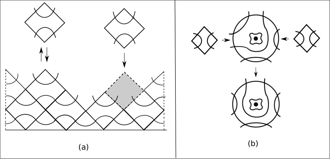 Figure 1
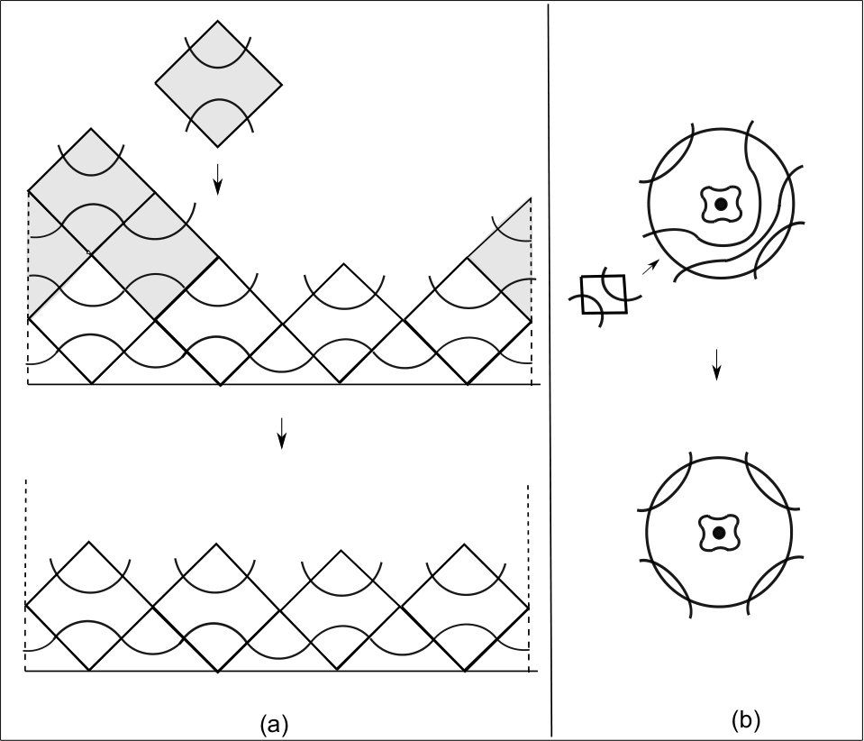 Figure 2
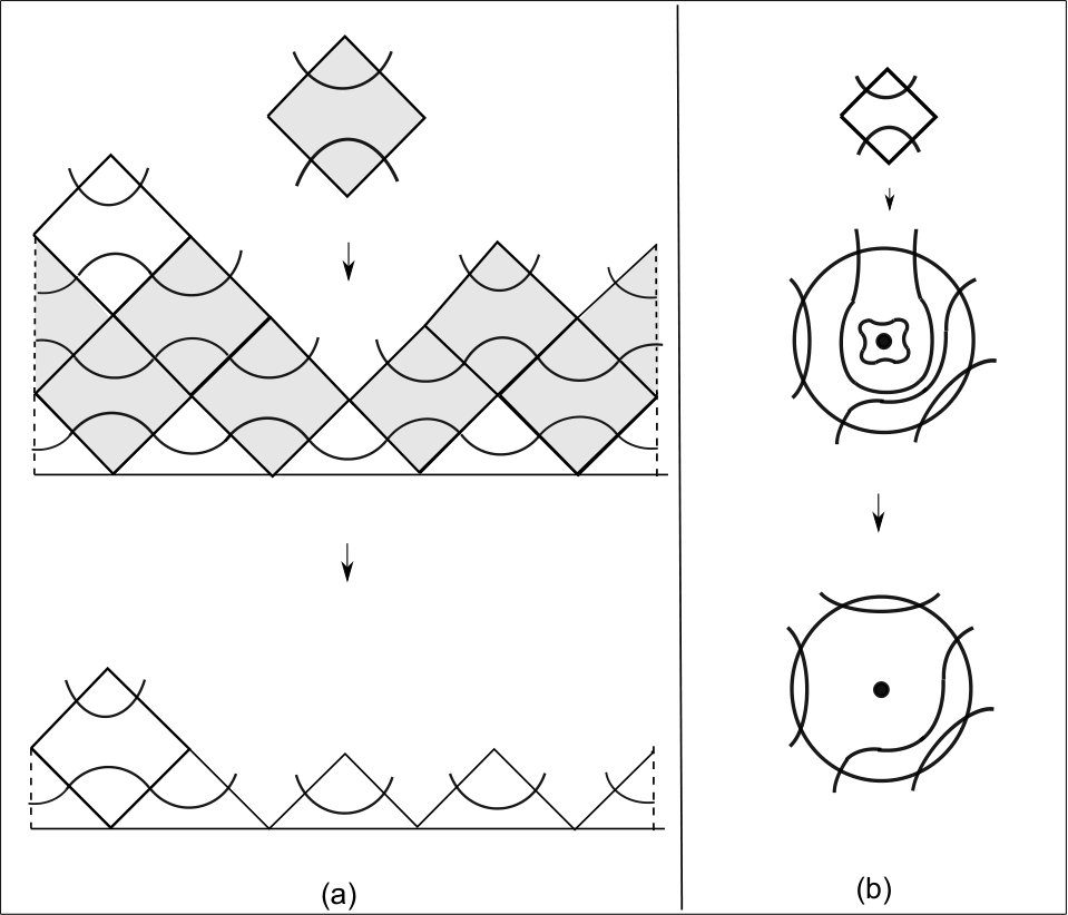 Figure 3
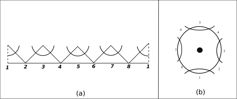 Figure 4
Peer Reviews
No public reviews on file for this paper yet. If you reviewed it on a platform where reviews are public (OpenReview, ICLR, NeurIPS, ICML), you can paste yours below so the community can read it here.
Videos
No videos yet. Explain this paper in a talk, walkthrough, or lecture? Add one.
Laws of large numbers in the Raise and Peel model
A.M. Povolotsky
Bogoliubov Laboratory of Theoretical Physics, Joint Institute for Nuclear Research, 141980, Dubna, Russia
National Research University Higher School of Economics, 20 Myasnitskaya, 101000, Moscow, Russia
Abstract
We establish the exact laws of large numbers for two time additive quantities in the Raise and Peel model, the number of tiles removed by avalanches and the number of global avalanches happened by given time. The validity of conjectures for the related stationary state correlation functions then follow. The proof is based on the technique of Baxter’s T-Q equation applied to the associated XXZ chain and on its solution at obtained by Fridkin, Stroganov and Zagier.
Keywords: law of large numbers, Temperley-Lieb algebra, Bethe ansatz, loop models, T-Q Baxter’s equation
1 Introduction
The Raise and Peel model (RPM) [1] is a non-equilibrium model of fluctuating interface defined as a continuous time Markov process. Its generator is given by a stochastic version of the Temperley-Lieb (TL) Hamiltonian [2], which in turn is a highly anisotropic limit of the transfer matrix of O(1) dense loop model. The general O(n) loop model has been intensively studied in context of theory of critical phenomena since it was introduced in [3] as a graphical lattice model expected to share the universality class with O(n) vector model. The interest to the particular case of O(1) dense loop model increased significantly after an observation by Razumov and Stroganov of a nice combinatorial structure in the ground state of an incarnation of the TL Hamiltonian, the XXZ quantum chain at a specific combinatorial point [4]. The further studies led to a discovery of the celebrated Razumov-Stroganov conjecture on a miraculous connection between the ground state of the O(1) dense loop transfer matrix and the set of configurations of the fully packed loop model, in turn related to the alternating sign matrices [5]. Also a number of conjectures on relations between RPM and the six vertex model, XXZ model, the fully packed loop model, the O(1) dense loop model and alternating sign matrices came from the studies of this subject. Some of these conjectures, including the Razumov-Stroganov conjecture itself [6], were proven and much more are still waiting for the proof (see [7, 8] and references therein).
Many statements concern the structure of the ground state vector of the transfer matrices or Hamiltonians under consideration. The term combinatorial point refers to the fact that at specific values of the parameters the coordinates of the ground state vector in a suitable basis can be normalized to be positive integers. Then the sums of these integers turned out to be related to combinatorial numbers coming from the enumeration of the alternating sign matrices. Treating the suitably normalized coordinates as a probability distribution one can also evaluate the marginal probabilities or the correlation functions over this distributions. Basing on the analysis of finite size systems several conjectures on exact ground state normalization and correlation functions of the O(1) dense loop model with different types of boundary conditions were proposed e.g. in [9, 10].
In the present paper we concentrate on the proof of two such conjectures in context of the RPM. Below we consider the RPM on the segment with periodic boundary conditions. The model is formulated in terms of 1-d interface, which is the upper boundary of the densely packed set of rhombic tiles placed onto a given substrate. It evolves by stochastic addition of new tiles coming onto the interface from above. Depending on the local shape of the interface at the place where the tile arrives, it either stays (adsorption) or leaves (reflection) or causes a non-local avalanche, which removes tiles from the current configuration (desorption). We distinguish global and local avalanches depending on whether they spread through the whole system or the do not respectively.
In the large time limit this stochastic process evolves towards the stationary state. The vector of stationary probabilities of each configuration is the eigenvector of the stochastic generator in the configurational basis corresponding to the largest eigenvalue equal to zero. The eigenvector components normalized to be the positive integers have nice combinatorial properties mentioned above. Several conjectures of combinatorial nature were proposed for the stationary state observables of RPM [1, 7] and some other predictions on space and time correlation functions were made with the use of conformal field theory [11, 12].
Recently, the evolution of the RPM was also analysed beyond the stationary state within the framework of the large deviation theory [13]. This theory allows one to study the statistics of the so called additive functionals on the trajectories of Markov processes in the large time limit. Two time-integrated quantities were studied: the number of all tiles removed within the avalanches by given time and the total number of global avalanches happened by the same time. In particular a few rescaled cumulants of these quantities were obtained asymptotically in the limit of large system to the second and first order in the inverse system size respectively. Note that in general the cumulants of time additive quantities depend non-trivially on unequal time correlations and, thus, can not be obtained from the stationary state observables. An exception is the first order cumulants, the mean values, which are related to specific stationary state observables, probabilities of events responsible for the change of the quantities under consideration. Indeed, the limiting time averages and were related to stationary probabilities of specific interface configurations, and were shown to match the leading orders of the previously conjectured exact expressions of these probabilities. The aim of the present paper is to establish the exact laws of large numbers for these quantities at an arbitrary system size and hence to prove the related conjectures for the stationary state correlation functions. Practically this means the exact calculation of the above limits, which suggest a convergence in expectation. Also, it is a simple fact from the theory of continuous-time finite Markov chains that the convergence in expectation can be upgraded to the almost sure convergence, which turns our statement to the strong laws of large numbers.
Technically, calculations of the exact stationary state averages require finding the stationary state probabilities explicitly, and, then, summing over them with the quantity being averaged. This is not an easy technical problem even on the level of finding the overall normalization factor, see e.g. [14]. However in the case of the observables related to the time-additive quantities the large deviation approach allows one to reduce the calculations, to the analysis of the largest eigenvalue of the deformed Markov generator rather than the eigenvector. This deformation suggests including counting parameters into the matrix of the generator, bringing the latter away from stochastic point. The largest eigenvalue of such a deformed generator becomes the scaled cumulant generating function of the time-additive quantities. The scaled cumulants, aka the derivatives of this eigenvalue with respect to the deformation parameters at zero (the stochastic point), can be obtained using the connection of the RPM to the XXZ model. To this end we use the technique based on solving the Baxter’s T-Q equation at the roots of unity developed in [15, 16]. Similar calculation were done in [17] for the nearest neighbor spin-spin correlation functions in XXZ model with periodic boundary conditions. In our case we make the calculations for the XXZ chain with twisted boundary conditions corresponding to the stochastic generator, with the twist being one of the counting deformation parameters. Note that in our case the stationary state correlation functions are defined in terms of the interface configurations, rather than in spin basis natural for the XXZ chain. The connection between these two bases is highly non-local [18], and in general the explicit relation between observables in XXZ chain and the RPM is very non-obvious.
The paper is organized as follows. In Section 2 we define the model, formulate the conjectures about two stationary state correlation functions and state the main result as a Theorem 1. We also discuss there the relation of the stationary state conjectures to the law of large numbers proved. In Section 3 we introduce the generator of the Markov process and the deformed generator in terms an operator in a finite dimensional ideal in the periodic Temperley-Lieb algebra and using its R-matrix representation reduce the problem to finding the largest eigenvalue of the XXZ chain with twisted boundary conditions. It is reformulated in terms of solving the system of algebraic Bethe ansatz equations. In the section 4 we rewrite the Bethe ansatz equations in form of T-Q relation and use the method of its solution developed in [15, 16] to calculate explicitly the derivatives of the eigenvalue. The subsections 4.2 and 4.3 contain the technical details of the calculation presented. We summarize the results and discuss some perspectives in section 5.
2 Raise and Peel model, problem statement and main result
2.1 Definition of the model
We consider the RPM on the segment of integer even length with periodic boundary conditions. The evolution starts from the substrate, which is the one-dimensional chain of rhombic tiles with the diagonals of the length 2. The right end of the segment is identified with the left end. The evolving random configuration is formed by adding tiles on top of this substrate. The evolution preserves the tiles of the substrate. This is why we picture only the upper halfs of tiles of the substrate above the middle line, which we refer to as zero level, see fig. 1a.
An independent Poissonian clock is associated with each integer horizontal position . The clock rings after an exponentially distributed waiting time with unit mean. When the clock at some position rings, a tile falls onto the system at this position causing the change of current configuration. The configuration of tiles established after such a change, the stable configuration, is densely packed below its upper boundary, the broken line, which makes steps either or , is forbidden to go down beyond the zero level and should touch the first level at least once. Following to [13] we refer to it as the periodic Dyck path (PDP), and to such a system representation as the PDP representation.
What happens, when the new tile arrives, depends on the local shape of the interface at the arrival position. If the tile arrives at the local maximum, the “peak”, it gets reflected, i.e. simply removed, see fig. 2a.
If the tile arrives at the local minimum, the “valley”, it gets absorbed, i.e. stays in the valley producing another stable configuration, except when the tile has completed two full layers of tiles on top of the substrate. In the latter case the configuration becomes unstable, and the global avalanche happens, which removes the two full layers of tiles including the arrived one, fig.3.
Arrival of the tile at the “slope of a mountain” also produces an unstable configuration, that relaxes by the local avalanche that peels off one layer of tiles at the level of arrival and upwards the mountain up to the same level at the opposite slope including the tile arrived, fig. 4. Local and global avalanches represent the non-local desorption events.
Another way to picture the process is to use the link representation. To go from the PDP to the link representation we supply every tile with a pair of links, one connecting between the bottom edges and the other between the top edges of the tile. Then, every configuration is represented by the non-crossing pairing of free ends of links directed upwards plus may be one loop going around the whole system. Arrival of new tiles causes rewiring of the free ends. The above rules of the dynamics of tiles suggest that a contractible loop appeared after the tile arrival must be contracted. As soon as a pair of non-contractible loops has appeared, it should be removed.
This picture becomes more clear, when projected onto the disk punctured in the center, see figs. 1b-4b. Then, a configuration is represented by either a directed non-crossing pairing of points on the boundary of the disk or such a pairing plus a non-contractible loop going around the hole in the center. The term directed [8] suggests that the hole allows one to define a unique direction of the links. Then, the pairings of points and , i.e. where the link either goes around the hole or not, are considered as different. As a new pair of links arrives, it causes a rewiring of the links, where all the contractible loops must be contracted. As a pair of non-contractible loops appears, they should be removed.
The link representation traces back to the O(1) model, which is the statistical physics model, defined as an ensemble of tilings of plain domains with rhombic tiles with two possible orientations of pairs of links connecting the adjacent edges. Each orientation of the tile is assigned a statistical weight. In the stochastic version of such a model the sum of the two weights is equal to one. The continuous time limit suggests that the weight of one orientation is infinitesimally small. The RPM in the PDP and in the link representation corresponds to the continuous time stochastic O(1) tiling of the half-plain, were we move through the tiling layer by layer, tracing only the connectivity of the ends of the links at a given layer and the odd-counted non-contractible loops. All the contractible loops fall out of consideration as well as the pairs of non-contractible loops. More on this connection see in [14].
There is yet another representation of RPM obtained from identifying every PDP with a configuration of particles on the one-dimensional lattice with sites. To this end, one uses the usual interface-particle system mapping. Every of steps or of PDP is identified with particle or hole, respectively. The dynamics of particles, which obey the exclusion interaction then follow from the RPM dynamics. This system was introduced and analyzed in [12], where it got a name “Nonlocal asymmetric exclusion process” NAEP due to nonlocal particle jumps, corresponding to the avalanches in the RPM.
2.2 Stationary state and laws of large numbers for the avalanche currents.
The above Markov process with finite state space having an irreducible transition matrix evolves towards the unique stationary state. As was discussed in the introduction, the vector of the stationary state probabilities, i.e. the eigenvector of the transition matrix corresponding to the non-degenerate zero eigenvalue, reveals nice combinatorial properties. In particular, it can be normalized so that its smallest component is one and the others are positive integers, whose sum is given by the number of the half-turn symmetric alternating sign matrices. Then many conjectures on correlation functions have simple rational form. Two conjectures we address here are as follows.
**Conjecture 1.**The average number of peaks (local maxima) as well as valleys (local minima) in the stationary state is
[TABLE]
Conjecture 2. Stable configurations which do not have valleys on level [math] and have a single valley on level appear in the stationary state with probability
[TABLE]
where we used the notation for the set of such configurations.
The first conjecture for the number of peaks was proposed in [14], where the subconfigurations corresponding to peaks were referred to as minimal one-nests. It is worth noting that conjectures similar to Conjecture 1 for RPM with different boundary conditions were proposed in [1, 19].
The second conjecture follows from the probability distribution of the number of nests in a configuration conjectured in [8]. Specifically the probability of configuration with a single nest, obtained from the conjectured expression, is twice larger than our value in (2). Pronounced in the language of link representation, the pairings considered in [8] ignore the presence of non-contractible loops. Thus, the configurations considered in [8] correspond to pairs of configurations in our system with and without non-contractible loop having the same connectivity structure and equal probability. Hence, the factor of separates those configurations with a non-contractible loop present, where a second loop appears after an addition of a single pair of links, like in fig. 3b.
The above stationary state correlation functions are related to the laws of large numbers for the avalanche currents and introduced in [13]. Below we argue that the conjectures are equivalent to the following theorem, which is the main result of this paper.
Theorem 1**.**
The following limits hold with probability one
[TABLE]
[TABLE]
The value (4) for the stationary state average current was conjectured by P. Pyatov basing of the direct evaluation of the stationary state eigenvector of the finite size transition matrices, and then applied to predict the mean current in the NAEP [12]. Both formulas were confirmed asymptotically in the leading orders in in [13].
To show the first connection let us introduce two other time integrated quantities - the total number of tiles arrived at the system and the number of tiles arrived at the peaks by the time . Then, we note that the total number of tiles arrived by the time is the number of tiles on top of the substrate at time plus the tiles reflected by the peaks and the tiles removed by avalanches, i.e
[TABLE]
We now note that is the usual Poisson process with the arrival rate . By the law of large numbers for the Poisson process, see e.g. [20], the limit
[TABLE]
holds almost surely, i.e. with probability one.
The process is an example of the so called doubly stochastic Poisson process or Cox process [21], i.e. the Poisson process with random arrival rate One can think of it as of the Poisson process with stochastic time . By ergodic theorem for Markov processes, see e.g. [22], the limit
[TABLE]
holds almost surely. Hence the law of large numbers for also takes place [23]
[TABLE]
with almost sure convergence. Finally, since is bounded as , the limit
[TABLE]
holds with probability one.
For the second conjecture we note that it gives exactly the probability of a configuration, where an addition of a single tile completes two full layers of tiles on top of the substrate. Thus is the doubly stochastic Poisson process with the random arrival rate , where is an indicator function of the set and is a random configuration at the time . Since by ergodicity
[TABLE]
the law of large numbers also holds for
[TABLE]
In the next sections we find the limits for convergence in expectation using the large deviation technique. As the almost sure convergence to a constant implies the convergence in expectation to the same limit, this proves the theorem 1 as well as the conjectures 1,2.
3 RPM, XXZ and the Bethe ansatz
Consider the periodic Temperley-Lieb algebra on [24] generated by operators satisfying the usual TL relations
[TABLE]
where , with the periodicity condition . The coefficient in (5) is the algebra coefficient parameterized by . We need its quotient algebra by relations
[TABLE]
where
[TABLE]
are the (unnormalized) projectors, and is an algebra parameter. Finally we consider the finite dimensional left ideal generated by the monomial . The monomials from this ideal can be visualized as the stable configurations of RPM read from left to right and from top to bottom, where the generator corresponds to the tile at horizontal position . Specifically, represents the substrate. The other stable configurations are obtained by multiplying by generators with subsequent reduction of the monomials by successive application of the relations (5-8). It is easy to see that up to the numerical factors, which are products of powers of and , the reduction is equivalent to the processes following the tile arrival described above . These factors turn to units at the stochastic point
[TABLE]
Then, the in the basis of monomials generated by the matrix of the operator
[TABLE]
is stochastic. It is a forward generator of the RPM Markov process, which describes the time evolution of the probability distribution of system configuration
[TABLE]
Here is a transition rate from a configuration to , which is either one or zero in the case of RPM.
Let us introduce a deformed generator depending on two parameters and with action
[TABLE]
which is obtained from by multiplying the off-diagonal matrix elements by where and are the increases of corresponding quantities and within the transition from the to . Its matrix coincides with the matrix of the operator
[TABLE]
in the monomial basis with the rescaled operators
[TABLE]
where we set
[TABLE]
The importance of this operator is due to the fact that its largest eigenvalue is the scaled joint cumulant generating function of and . In particular
[TABLE]
For further details see [13].
3.1 Bethe ansatz
The further solution for the largest eigenvalue is based on the use of the R-matrix representation of the PTLL on the space . In this space the generator can be represented by
[TABLE]
where and are the matrices
[TABLE]
acting in the -th copy of and the parameters and are related to and by
[TABLE]
Then the representation of the deformed Markov generator
[TABLE]
is expressed in terms of the Hamiltonian
[TABLE]
of the anti-ferromagnetic Heisenberg quantum chain of spins 1/2 with anisotropy . Note that by a unitary transformation the parameter can be transferred from the Hamiltonian to twisted boundary conditions:
[TABLE]
Finally, the largest eigenvalue of the operator is
[TABLE]
where is the groundstate eigenvalue of found in the sector isomorphic to the ideal
The eigenvalues of in the sector , where are given in terms of solutions of the system of Bethe ansatz equations (BAE)
[TABLE]
Then, the energy corresponding to a particular solution is
[TABLE]
Making a variable change
[TABLE]
we obtain
[TABLE]
and
[TABLE]
As a result, for the rescaled cumulant generating function of avalanche currents in RPM we obtain
[TABLE]
where we should set . To proceed with the proof of the statements of interest we need to identify the groundstate solution of the system of BAE for and to evaluate the derivatives of with respect to and (i.e. with respect to and ) at the stochastic point corresponding to
[TABLE]
The necessary technique based on the T-Q equation was developed by Fridkin, Stroganov, Zagier (FSZ) in [15, 16].
4 Bethe ansatz equations as T-Q relation
The system of BAE can be rewritten as a single functional relation for the polynomial
[TABLE]
with the roots being the root of a particular solution of BAE.
Then the BAE then read as
[TABLE]
Where we introduce a notation
[TABLE]
This T-Q relation is obtained as a condition of divisibility of the degree polynomial in the r.h.s. by . The ratio is the polynomial of degree , which is known to be the eigenvalue of the transfer matrix of the corresponding asymmetric six-vertex model [25]. The eigenvalues (17) of XXZ Hamiltonian can be expressed in terms of either or at specific points, which yields the following formulas for
[TABLE]
It is also worth noting that multiplying the Bethe equations, we obtain
[TABLE]
For every state we should choose one of roots of unity for the product The groundstate Bethe vector is translationally invariant, so that the corresponding solution satisfies to
[TABLE]
i.e.
[TABLE]
which, being used in relation (19) at , yields
[TABLE]
4.1 FSZ solution.
The formulas of the previous subsection were valid for arbitrary and . From now on we imply that and write everything in terms of for simplicity. Since we use multiplicative parametrization rather than the additive of [15, 16], to be self-contained we briefly sketch the arguments of those papers. Let us introduce notations
[TABLE]
It follows from (19)
[TABLE]
When , these are periodic functions
[TABLE]
For this system to have a solution for the rank of the matrix
[TABLE]
should be less than 3. It was observed that at the stochastic point there is a unique solution for that makes the rank of the matrix equal to one
[TABLE]
that luckily corresponds to the groundstate solution of BAE of the XXZ model with Substituting
[TABLE]
we obtain a q-difference equation for
[TABLE]
To solve this equation we introduce function
[TABLE]
which is a polynomial of degree
[TABLE]
In terms of this function the relation (24) reads as
[TABLE]
This relation fixes out of coefficients . The remaining coefficients can be found up to overall normalization factor from the condition that has a zero of order at This fact is used as follows. We require vanishing the derivatives of up to order at
[TABLE]
for As shown in [15, 16] this can be satisfied by finding numbers
[TABLE]
such that for any polynomial of degree the linear combination of its evaluations at points with these coefficients vanishes.
[TABLE]
In this way we define only up to a common factor
[TABLE]
Substituting this to we obtain
[TABLE]
where
[TABLE]
is the Pochhammer symbol, and we choose the common factor such that the largest degree coefficient is The latter condition follows from our normalization of as .
One can see that the system of BAE is invariant with respect to the simultaneous transformation and This suggests that for every solution of BAE there exists a solution of another system obtained form the original one by the change , which corresponds to a parity transformation. The analogue of in that case will be
[TABLE]
Such a polynomial solves the equation obtained from (19) by the change and The symmetry corresponds to the simultaneous spin and space reversal symmetry of the transfer matrix [25], which in turn suggests the equation for
[TABLE]
Note that the further calculation does not explicitly use arguments based on the interpretation of as a transfer matrix eigenvalue. What we need is the solution of (29) with the same as in (19). However, the argument is what ensures the existence of such a solution.
Similarly to , at the stochastic point the polynomial can be found in the form
[TABLE]
where
[TABLE]
For arbitrary and the two polynomials satisfy a Wronskian-like relation
[TABLE]
and the polynomial can be written in terms of them
[TABLE]
4.2 Calculating derivatives
Lastly we need to evaluate the derivatives of at and
4.2.1 The first argument
For the derivative in we have
[TABLE]
where we suggest that , the subscript means the partial derivative in at we taken into account that and follows from (20,22). Therefore we need to calculate , differentiating in the argument and in and the substituting Calculating the derivatives of (31) and (32) at and respectively we obtain
[TABLE]
where
[TABLE]
Eliminating between (34) and (35) we obtain
[TABLE]
Thus, we have reduced the problem to calculation of the values of and and their first derivatives at
4.2.2 The second argument.
For the derivative in we have
[TABLE]
To calculate we use (23) and for the derivative we differentiate (21) in . The difficult part is to find . To this end we differentiate (32) with respect to which yields
[TABLE]
where the subscript indicates that the expression in the brackets is obtained by interchanging the polynomials and and
[TABLE]
Then from (31) we obtain
[TABLE]
where we find that
[TABLE]
which finally yields
[TABLE]
Thus, we again have reduced the problem to evaluation of the values of and and their derivatives up to the second order at points
4.3 Calculations with and
Below we obtain the necessary values of and and their derivatives. After substituting them to the formulas (4.2.1-37) and lengthy but straightforward algebra we obtain the following results
[TABLE]
which prove Theorem 1.
The result of this section is as follows.
[TABLE]
[TABLE]
[TABLE]
[TABLE]
To evaluate the values and the derivatives of and at we use their representation (25,30) in terms of functions and .
I. At we represent these functions in terms of the Gauss hypergeometric functions
[TABLE]
[TABLE]
Then using the fact that the Chu-Vandermonde identity for evaluating the hypergeometric function at the unit variable with being positive integer, and the formula of a derivative of the hypergeometric function we obtain stated formulas.
II. At the same problem is more delicate as the functions and have zeros of multiplicity at this point. Let us proceed with the calculation for which will also give us the results for with use of the relation (28). Calculating the derivatives of (25) and setting we obtain
[TABLE]
We need to evaluate for Let us introduce the notation
[TABLE]
Now we prove the identities
[TABLE]
which being substituted to (38) yields the above stated results. To prove the identities, we show that their l.h.s divided by the r.h.s. is a difference of two parts, which satisfy the same recurrent relations with respect to . As their initial values differ by one, the ratios are equal to one. To establish the recursion we use the Maple implementation of Zeilberger’s algorithm of finding the recurrent relations for hypergeometric-like sums [27].
a) For the first identity we have
[TABLE]
where
[TABLE]
with convention for The quantities and satisfy the same recurrent relation
[TABLE]
with initial conditions
b) For the second identity
[TABLE]
[TABLE]
The recursion for and is
[TABLE]
with initial conditions
c)
[TABLE]
[TABLE]
The recursion for and is
[TABLE]
with initial conditions
5 Conclusion
To summarize, we obtained the exact expressions for the avalanche currents in the Raise and Peel and justified the previous conjectures. This task was completed by using the large deviation arguments, which reduce the calculation to evaluation of the derivatives of the largest eigenvalue of the deformed generator of the process. Technically, the eigenvalue of the transfer matrix both in spectral parameter and in the twist parameter or in the quantum group parameter was calculated. This work can be considered as the first step towards the construction of the exact large deviation function of the avalanche currents, which was obtained asymptotically for the large system size in [13]. In particular, the next step would be obtaining the second cumulants, the diffusion coefficients and the mutual covariance of the two currents. While their asymptotic expressions were obtained in [13], conjectures on exact expressions like those for the mean currents are absent. Will the technique used here still be applicable in that case is a question for further studies. Also it would be interesting to find other currents, whose statistics could be studied in the same way, e.g. the ones related to spectral parameters in nonuniform Bethe ansatz.
We dedicate this work to Vladimir Rittenberg, our colleague and friend who was always an inexhaustible source of questions, who inspired us and motivated the work on this project. We are grateful to Pavel Pyatov for useful discussions. The work is supported by Russian Foundation of Basic Research under grant 17-51-12001 and by the HSE University Basic Research Program jointly with Russian Academic Excellence Project ’5-100’.
The reference list from the paper itself. Each links out to its DOI / PubMed record.
- 1[1] De Gier J, Nienhuis B, Pearce P A and Rittenberg V 2004 Phys. 114 1
- 2[2] Temperley H N V and Lieb E 1971 Proc. R. Soc . A 322 251
- 3[3] Domany E, Mukamel D, Nienhuis B and Schwimmer A 1981 Nucl. Phys. B 190 279 .
- 4[4] Razumov A V and Stroganov Yu G 2001 J. Phys. A: Math. Gen. 34 3185-3190.
- 5[5] Razumov A V and Stroganov Yu G 2004 Theor. Math. Phys. 138 333
- 6[6] Cantini L and Sportiello A 2011 J. Comb. Theor. A 118 1549
- 7[7] Alcaraz F C and Rittenberg V 2007 J. Stat. Mech. P 07009.
- 8[8] de Gier J 2005 Discr. Math. 298 365