The $B$ Anomalies and New Physics in $b \to s e^+ e^-$
Alakabha Datta, Jacky Kumar, David London

TL;DR
This paper explores how new physics contributions to both muon and electron channels in $b o s \, \ell^+ \ell^-$ decays can resolve tensions in explaining the $B$ anomalies, especially in light of recent $R_K$ measurements.
Contribution
It investigates the impact of new physics in $b o s e^+ e^-$ on existing $b o s \mu^+ \mu^-$ anomalies, proposing scenarios with combined contributions to improve data fits.
Findings
Adding NP in $b o s e^+ e^-$ can improve fit quality.
Models with contributions to both muon and electron channels are viable.
Future measurements may require multi-particle NP models.
Abstract
We investigate the implications of the latest LHCb measurement of for NP explanations of the anomalies. The previous data could be explained if the NP is in (I) or (II) , with scenario (I) providing a better explanation than scenario (II). This continues to hold with the new measurement of . However, for both scenarios, this measurement leads to a slight tension of between separate fits to the and data. In this paper, we investigate whether this tension can be alleviated with the addition of NP in . In particular, we examine the effect of adding such NP to scenarios (I) and (II). We find several scenarios in which this leads to improvements in the fits. and LQ models with contributions to both $b \to s…
Click any figure to enlarge with its caption.
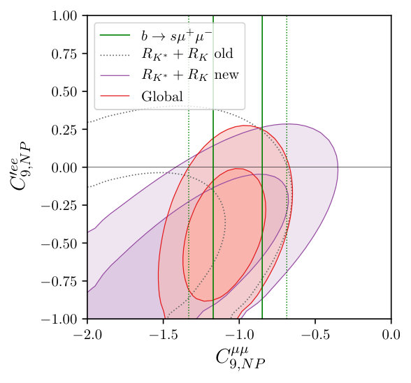 Figure 1
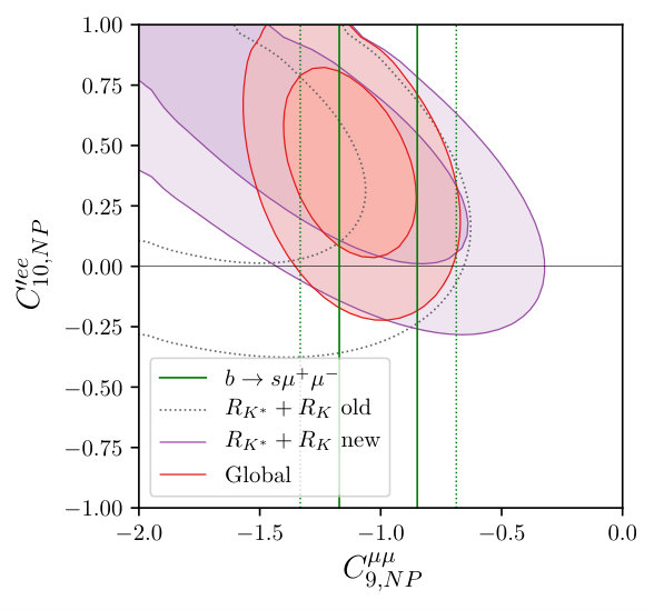 Figure 2
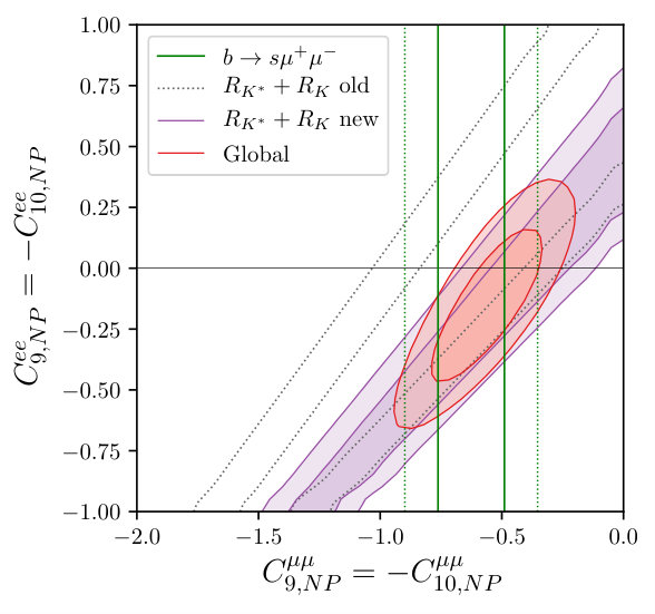 Figure 3
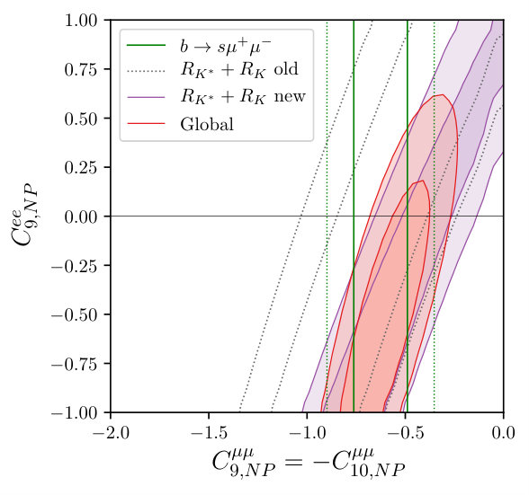 Figure 4
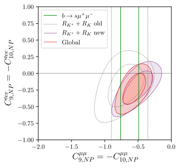 Figure 5
| Scenario | WC | p-value | pull |
|---|---|---|---|
| (I) | 0.71 | 5.8 | |
| (II) | 0.64 | 5.5 |
| Scenario | Data Set | WC |
|---|---|---|
| (I) | ||
| (II) | ||
| NP in | p-value | Pull | ||
|---|---|---|---|---|
| S0 | 0.73 | 5.8 | ||
| S1 | 0.77 | 6.0 | ||
| S2 | 0.76 | 5.9 |
| NP in | p-value | Pull | ||
|---|---|---|---|---|
| S3 | 0.65 | 5.6 | ||
| S4 | 0.69 | 5.7 | ||
| S5 | 0.67 | 5.6 |
| LQ | ||||
|---|---|---|---|---|
| 0 | 0 | |||
| 0 | 0 | 0 | ||
| 0 | 0 | |||
| 0 | 0 | |||
| 0 | 0 | 0 |
| Field | Operators | Field | Operators |
|---|---|---|---|
| Coloured Spin-0 | -singlet | , | |
| -singlet | Vector Boson | ||
| Coloured Spin-0 | -doublet | ||
| -doublet | Vector Boson | ||
| Coloured Spin-0 | -triplet | ||
| -triplet | Vector Boson | ||
| Exotic Quark: | Coloured Spin-1 | ||
| Vector-singlet | -singlet | ||
| Exotic Quark: | Coloured Spin-1 | ||
| Vector-doublet | -doublet | ||
| Exotic Quark: | Coloured Spin-1 | ||
| Vector-triplet | -triplet |
Peer Reviews
No public reviews on file for this paper yet. If you reviewed it on a platform where reviews are public (OpenReview, ICLR, NeurIPS, ICML), you can paste yours below so the community can read it here.
Videos
No videos yet. Explain this paper in a talk, walkthrough, or lecture? Add one.
UdeM-GPP-TH-19-270
The Anomalies and New Physics in
Alakabha Datta *a,*[email protected], Jacky Kumar *b,*[email protected] and David London *b,*[email protected]
: *Department of Physics and Astronomy, 108 Lewis Hall,
* *University of Mississippi, Oxford, MS 38677-1848, USA
* : *Physique des Particules, Université de Montréal,
* C.P. 6128, succ. centre-ville, Montréal, QC, Canada H3C 3J7
()
Abstract
We investigate the implications of the latest LHCb measurement of for NP explanations of the anomalies. The previous data could be explained if the NP is in (I) or (II) , with scenario (I) providing a better explanation than scenario (II). This continues to hold with the new measurement of . However, for both scenarios, this measurement leads to a slight tension of between separate fits to the and data. In this paper, we investigate whether this tension can be alleviated with the addition of NP in . In particular, we examine the effect of adding such NP to scenarios (I) and (II). We find several scenarios in which this leads to improvements in the fits. and LQ models with contributions to both and can reproduce the data, but only within scenarios based on (II). If the tension persists in future measurements, it may be necessary to consider NP models with more than one particle contributing to .
At present, there are several measurements of -decay processes involving the transition () that are in disagreement with the predictions of the standard model (SM). First, there are discrepancies with the SM in a number of observables in [1, 2, 3, 4, 5] and [6, 7], decays which involve only . Second, the measurements of [8] and [9] also disagree with the SM predictions. These ratios involve both and . In this paper, we refer to these two sets of observables as the and observables.
Since all processes involve , it is natural to examine whether the anomalies can be explained by adding new physics (NP) to this decay. The transitions are defined via an effective Hamiltonian with vector and axial vector operators:
[TABLE]
where the are elements of the Cabibbo-Kobayashi-Maskawa (CKM) matrix and the primed operators are obtained by replacing with . The Wilson coefficients (WCs) include both the SM and NP contributions: . Following the announcement of the measurement in 2017, global fits were performed that combine the various observables [10, 11, 12, 13, 14, 15, 16, 17]. It was found that the net discrepancy with the SM is at the level of 4-6, and that the data can be explained if the nonzero WCs are (I) or (II) . In Ref. [17], the best-fit values of the WCs for these two scenarios were found to be (I) and (II) (other analyses found similar results). The simplest NP models involve the tree-level exchange of a leptoquark (LQ) or a boson. Scenario (II) can arise in LQ or models, but scenario (I) is only possible with a [17].
The first measurement of was made in 2014 by the LHCb Collaboration using the Run 1 data [8]. For , where is the dilepton invariant mass-squared, the result was
[TABLE]
This differs from the SM prediction of [18] by . Recently, LHCb announced new results [19]. First, the Run I data was reanalyzed using a new reconstruction selection method. The new result is
[TABLE]
Second, the Run 2 data was analyzed:
[TABLE]
Combining the Run 1 and Run 2 results, the LHCb measurement of is
[TABLE]
This is closer to the SM prediction, though the discrepancy is still due to the smaller errors.
The LHCb measurement of was [9]
[TABLE]
Recently, Belle announced its measurement of [20]:
[TABLE]
The errors are considerably larger than in the LHCb measurement.
In this paper we examine the effect of these new measurements – especially that of [Eq. (5)] – on the NP explanations of the anomalies.
The first step is to simply combine all the observables, and update the global fit performed in Ref. [17]. (We refer to this paper for a description and the measured values of all the (CP-conserving) observables.) This is done using the programs MINUIT [21, 22, 23], flavio [24] and Wilson [25]. The results are shown in Table 1.
For each scenario we present the best-fit value of the WCs, as well as the p-value and the pull:
The p-value is derived from and characterizes the goodness of fit. If all observables were “clean,” i.e., if the theoretical error associated with their predictions were small, then the dominant error in the fit would be purely statistical. In this case, the distribution would be Gaussian, with a central value of 1, corresponding to a p-value of 0.5. In general, it is assumed that, if the fit produces a p-value of (i.e., outside the 95% C.L. region), this is considered to be an unacceptable fit.
Usually, one does not compare the p-values of different fits – a fit is either acceptable or it is not. However, in this paper, we are interested in determining whether a particular (acceptable) scenario provides a better description of the data than another (acceptable) scenario, and so we will compare the p-values. (Admittedly, the difference in the p-values of two acceptable scenarios is not statistically significant.)
In the present fit, the observables are not clean: all of them involve sizeable theoretical uncertainties (form factors), and each analysis of the anomalies has its own method of treating these theoretical errors. (In this paper, we take the theoretical uncertainties into account following Ref. [26].) However, the point is that the way these theoretical errors are estimated affects the results of the fit: methods with large (small) theoretical errors will tend to have larger (smaller) p-values. Thus, it makes no sense to compare the p-values of analyses that use different methods of dealing with the theoretical uncertainties. On the other hand, what is rigorous is to compare the p-values of scenarios that use the same theoretical method. We therefore conclude that scenario (I) (p-value = 0.71) provides a slightly better explanation of the data than scenario (II) (p-value = 0.64). And both are enormous improvements on the SM, which has a p-value of 0.05. 2. 2.
The pull is defined to be , i.e., it quantifies how much better the SM + NP fit is than the fit with the SM alone. In the present case, since both scenarios involve only one free parameter, a pull of 5.8 indicates that (i) the discrepancy between the experimental data and the predictions of the SM is at least , and (ii) the addition of NP improves the agreement with the measurements by . From the p-values, we already concluded that scenario (I) explains the data somewhat better than scenario (II); in Table 1, this is reflected in a larger pull. Of course, this does not exclude the possibility of finding an even larger improvement over the SM in another NP scenario.
While this is an interesting result, the global fit does not contain all the important NP implications of the experimental data. Let us instead separate the data into and observables, and perform separate fits on these two data sets. The results are shown in Table 2. We see that there is now a slight tension between the NP WCs required to explain the and data: in scenario (I), the two best-fit values differ by , while in scenario (II) the difference is , where is defined by adding the errors of the two solutions in quadrature. The most obvious explanation of this tension is that it is simply a statistical fluctuation. However, in this paper, we investigate whether the tension can be alleviated with the addition of NP in . With this in mind, we consider a variety of scenarios in which some NP WCs are taken to be nonzero, in order to see if this tension can be removed, and the fit improved. As we will see, there are a number of scenarios with NP in in which this occurs.
In a recent paper [27], a similar observation was made about the different NP implications of the and data. And in Ref. [29], it was argued that a better description of the data can be obtained if one adds NP to the NP already assumed to be present in WCs. However, in both Refs. [27] and [29], rather than focusing on additional NP in and/or , there the analysis is done in terms of lepton-flavour-universal (LFU) and lepton-flavour-universality-violating (LFUV) NP. This same type of language is used in Ref. [30]. There it is argued that, when one includes the latest and measurements in the fit, a better description of the data is obtained if one has additional LFU NP. One of the points of the present paper is to note that this is not the only possibility. Here we show that additional NP in , which is clearly LFUV NP, can also lead to a better description of the data.
We begin by investigating the addition of NP in to scenario (I). We examine three different scenarios, shown in Table 3. In scenario S0, the best-fit value of the WC is consistent with zero, as in Table 1. This is reflected in the fact that the pull is also unchanged from Table 1. Thus, S0 is no better than the original scenario (I), and we discard it. On the other hand, in scenarios S1 and S2, nonzero values of the WCs are preferred. Furthermore, these scenarios are clear improvements, as is indicated by the increased p-values and pulls. These scenarios demonstrate that, by adding NP to , one can improve the agreement with the data.
For scenarios S1 and S2, in Fig. 1 we show the allowed and regions of the and new observables individually, as well as the combined fit, all as functions of the WCs. In both cases, we see that the combined global fit prefers nonzero values of the WC. We also see how the new measurement of has moved the parameter space of the combined fit.
We now add NP in to scenario (II). The three different scenarios considered are shown in Table 4. In all cases, there is an improvement in the fits compared to Table 1.
We therefore see that, with the addition of NP in , scenarios S3-S5 show an improvement over scenario (II) of Table 1. Still, even in the best case (S4), where the p-value and pull increase to 0.69 and 5.7, respectively, one still does not quite reach the level of scenario (I) without the addition of NP in (Table 1). That is, even if we allow for NP in , scenario (I) continues to provide a better explanation of the data than scenario (II). Even so, solutions S3-S5 are in no way ruled out, and so should not be discarded. In Fig. 2 we show the allowed regions of the S3, S4 and S5 scenarios in the parameter space of the WCs.
We now turn to a model-dependent analysis. As noted earlier, the simplest NP models that contribute to involve the tree-level exchange of a boson [scenario (I) or (II)] or a LQ [scenario (II) only]. With the previous data, both of these NP models were viable. Does this still hold with the present data? We begin by looking at LQs.
There are three types of LQ that can contribute to at tree level and involve only left-handed particles (). They are an -triplet scalar (), an -singlet vector (), and an -triplet vector () [32]. Their couplings are
[TABLE]
Here, in the fermion currents and in the subscripts of the couplings, and represent left-handed quark and lepton doublets, respectively, while , and represent right-handed up-type quark, down-type quark and charged lepton singlets, respectively. The LQs can couple to fermions of any generation. To specify which particular fermions are involved, we add superscripts to the couplings. For example, is the coupling of the LQ to a left-handed (or ) and a left-handed (or ). These couplings are relevant for or (and possibly ).
In LQ models, there may be contributions to lepton-flavour-conserving operators in addition to () [Eq. (1)]. They are
[TABLE]
contributes to , while and are additional contributions to . There may also be contributions to the lepton-flavour-violating (LFV) operators
[TABLE]
where , with . , and contribute to and . Using the couplings in Eq. (8), one can compute which WCs are affected by each LQ. These are shown in Table 5 for [33], and it is straightforward to change one or both to an . Finally, there may also be a 1-loop contribution to the LFV decay :
[TABLE]
All LFV operators can arise if there is a single LQ that couples to both and . Since the constraints from LFV processes are extremely stringent, we therefore anticipate that it may be difficult for a single LQ to both explain the anomalies via couplings to and and satisfy the LFV constraints.
The analysis of the LQ models has the following ingredients:
- •
and : All LQs have , . In principle, the LQ could also produce . However, if these primed WCs are sizeable, so too are the scalar WCs and (see Table 5). Now, the scalar operators [Eq. (9)] contribute significantly to [34]. The present measurement of [35, 36], in agreement with the SM, and the upper bound (90% C.L.) [37] constrain to be small.
- •
: As can be seen in Table 5, the and LQs can have nonzero WCs, so there may be additional constraints from . However, it was shown in Ref. [38] that the present constraints from are rather weak, and do not place significant limits on the WCs.
- •
LFV processes: The contributions of LQs to LFV processes were examined in detail in Ref. [28]. It was found that the most important LFV process is , with (90% C.L.) [37]. Even though the LQ contributes only at the 1-loop level, the very small upper limit on the branching ratio places stringent constraints on the model. The relevant WCs are [39]
[TABLE]
where , is given in the caption of Table 5, and , 2 and for the , and LQ models, respectively. In computing the constraints on the LQ models from , we conservatively take , as it leads to the weakest constraints.
Given that LQs can only contribute to , , the only one of the scenarios in Tables 3 and 4 that can be generated by LQs is S3, which is based on scenario (II). Indeed, the S3 and LQ fits are quite similar, except that there is an additional constraint on LQ models from . We find that all three LQ models can explain the data, with pulls of 5.6 (), 5.5 (), and 5.5 (). The pulls are very slightly lower than that of S3, due to the additional constraint. We therefore conclude that, with the new data, explanations of the anomalies involving a single LQ with contributions to both and are still possible, though they do not reproduce the data quite as well as NP scenarios based on scenario (I) (i.e., S1 amd S2).
We now turn to models. As was the case for LQs, other processes may be affected by exchange, and these produce constraints on the couplings. In particular, the coupling is constrained by - mixing and the coupling is constrained by the production of pairs in neutrino-nucleus scattering, (neutrino trident production). These constraints are discussed in detail in Ref. [28]. There it is found that, when these constraints are taken into account, the expected sizes of the NP WCs are |C_{9,10,{\rm NP}}^{(\prime)\mu\mu}|\mathrel{\raise 1.29167pt\hbox{<\kern-7.5pt\lower 4.30554pt\hbox{\sim}}}0.6.
In the most general case, the couplings of the to the various pairs of fermions are independent. For and transitions, the couplings that interest us are , , , , and , which are the coefficients of , , , , and , respectively. Defining and , we can then write
[TABLE]
where is given in the caption of Table 5.
With these expressions, it is straightforward to see that scenarios S1, S2 and S5 of Tables 3 and 4 cannot be produced with a . On the other hand, scenarios S3 and S4 can (scenario S0 can as well, but it has been discarded). Both scenarios require and , while scenario S3 (S4) requires (). In addition, the WCs roughly satisfy |C_{9,10,{\rm NP}}^{(\prime)\mu\mu}|\mathrel{\raise 1.29167pt\hbox{<\kern-7.5pt\lower 4.30554pt\hbox{\sim}}}0.6, which is required by the constraints from - mixing and neutrino trident production. This shows that scenarios S3 and S4 can be generated in a model with a gauge boson. Still, S3 and S4 are part of scenario (II), which does not explain the data quite as well as scenario (I).
To summarize, the NP models containing a single new particle that contributes to at tree level – LQ models and models with a – can both explain the present data if there are contributions to both and . However, in both cases, the nonzero WCs are [scenario (II)], and this does not provide quite as good a fit to the data as those scenarios with only . This leads one to consider the possibility of more than one NP contribution. Indeed, realistic NP models often contain a variety of new particles. To investigate the possibilities, it is useful to approach this question from the SM Effective Field Theory (SMEFT) [40, 41] point of view.
Any NP model must respect the gauge symmetries of the SM. When this NP is integrated out, one produces operators involving only the SM particles, but these must also be invariant under the SM symmetries. There are, of course, many possible operators, but we are interested only in those that contribute to the WCs ( or ) at low energy. Restricting ourselves to dimension-six NP operators that contribute to at tree level, there are two categories. First, there are four-fermion operators:
[TABLE]
Second, there are operators involving the Higgs field:
[TABLE]
The WCs can be written in terms of the coefficients of these operators [42]. The NP four-fermion operators generate
[TABLE]
and
[TABLE]
The and WCs are not necessarily equal, so these are LFUV NP contributions. (These have been studied in Ref. [16].) The operators involving the Higgs field generate LFU NP contributions:
[TABLE]
The and WCs can be treated similarly, but we note that they are not independent in SMEFT [33].
Thus, if one wishes to generate a particular WC, the above indicates which NP operators are required. The last step is to establish which types of NP particules can generate these NP operators. This was examined in Ref. [43]. In Table 6, we present the list of all types of NP particles and the operators that they generate. This allows model builders to work out exactly WCs are generated in a particular model. Conversely, if one wishes to generate only a particular WC, one can compute which combinations of particles are necessary to do this.
To conclude, in this paper we have examined the NP implications of the latest measurements of and . The result is particularly important. There are two sets of observables: (i) those involving only decays, and (ii) , which involve both and transitions. If a global fit to all data is performed, assuming new physics only in , it is found that (i) there is still a sizeable (5-6) discrepancy between the experimental results and the predictions of the SM, and (ii) this type of NP can explain it. However, if one looks more closely and performs separate fits to the and data, there is now a slight tension: the two fits give results that differ by . This may well be simply a statistical fluctuation, but here we examine whether the addition of NP in can reduce the tension.
It has been shown model-independently that the previous data could be explained by the addition of NP in (I) or (II) , with scenario (I) providing a better explanation than scenario (II). We considered the addition of NP in to these scenarios to see if the agreement with the present data can be improved. We identified several scenarios in which the addition of nonzero WCs to (I) or (II) resulted in such improvements. It has been argued elsewhere [30] that an improved agreement with the data can be obtained if there is additional lepton-flavour-universal NP. Our results show that this is not the only possibility: additional NP in , which is clearly lepton-flavour-universality-violating NP, can also do the job.
We also performed a model-dependent analysis. For NP models that involve the tree-level exchange of a single particle (LQ models and models with a ), we showed that they could explain the data, but only within scenarios based on (II). Since scenarios based on (I) provide a slightly better explanation of the data, it may be that more than one NP particle is contributing to . Using an SMEFT approach, we identify which NP operators contribute to at tree level, and what types of NP particles lead to these operators. This will permit the building of models that generate the desired and WCs.
Acknowledgments: This work was financially supported in part by NSERC of Canada (JK, DL).
The reference list from the paper itself. Each links out to its DOI / PubMed record.
- 1[1] R. Aaij et al. [LH Cb Collaboration], “Measurement of Form-Factor-Independent Observables in the Decay B 0 → K ∗ 0 μ + μ − → superscript 𝐵 0 superscript 𝐾 absent 0 superscript 𝜇 superscript 𝜇 B^{0}\to K^{*0}\mu^{+}\mu^{-} ,” Phys. Rev. Lett. 111 , 191801 (2013) doi:10.1103/Phys Rev Lett.111.191801 [ar Xiv:1308.1707 [hep-ex]].
- 2[2] R. Aaij et al. [LH Cb Collaboration], “Angular analysis of the B 0 → K ∗ 0 μ + μ − → superscript 𝐵 0 superscript 𝐾 absent 0 superscript 𝜇 superscript 𝜇 B^{0}\to K^{*0}\mu^{+}\mu^{-} decay using 3 fb -1 of integrated luminosity,” JHEP 1602 , 104 (2016) doi:10.1007/JHEP 02(2016)104 [ar Xiv:1512.04442 [hep-ex]].
- 3[3] A. Abdesselam et al. [Belle Collaboration], “Angular analysis of B 0 → K ∗ ( 892 ) 0 ℓ + ℓ − → superscript 𝐵 0 superscript 𝐾 ∗ superscript 892 0 superscript ℓ superscript ℓ B^{0}\to K^{\ast}(892)^{0}\ell^{+}\ell^{-} ,” ar Xiv:1604.04042 [hep-ex].
- 4[4] ATLAS Collaboration, “Angular analysis of B d 0 → K ∗ μ + μ − → superscript subscript 𝐵 𝑑 0 superscript 𝐾 superscript 𝜇 superscript 𝜇 B_{d}^{0}\to K^{*}\mu^{+}\mu^{-} decays in p p 𝑝 𝑝 pp collisions at s = 8 𝑠 8 \sqrt{s}=8 Te V with the ATLAS detector,” Tech. Rep. ATLAS-CONF-2017-023, CERN, Geneva, 2017.
- 5[5] CMS Collaboration, “Measurement of the P 1 subscript 𝑃 1 P_{1} and P 5 ′ subscript superscript 𝑃 ′ 5 P^{\prime}_{5} angular parameters of the decay B 0 → K ∗ 0 μ + μ − → superscript 𝐵 0 superscript 𝐾 absent 0 superscript 𝜇 superscript 𝜇 B^{0}\to K^{*0}\mu^{+}\mu^{-} in proton-proton collisions at s = 8 𝑠 8 \sqrt{s}=8 Te V,” Tech. Rep. CMS-PAS-BPH-15-008, CERN, Geneva, 2017.
- 6[6] R. Aaij et al. [LH Cb Collaboration], “Differential branching fraction and angular analysis of the decay B s 0 → ϕ μ + μ − → superscript subscript 𝐵 𝑠 0 italic-ϕ superscript 𝜇 superscript 𝜇 B_{s}^{0}\to\phi\mu^{+}\mu^{-} ,” JHEP 1307 , 084 (2013) doi:10.1007/JHEP 07(2013)084 [ar Xiv:1305.2168 [hep-ex]].
- 7[7] R. Aaij et al. [LH Cb Collaboration], “Angular analysis and differential branching fraction of the decay B s 0 → ϕ μ + μ − → subscript superscript 𝐵 0 𝑠 italic-ϕ superscript 𝜇 superscript 𝜇 B^{0}_{s}\to\phi\mu^{+}\mu^{-} ,” JHEP 1509 , 179 (2015) doi:10.1007/JHEP 09(2015)179 [ar Xiv:1506.08777 [hep-ex]].
- 8[8] R. Aaij et al. [LH Cb Collaboration], “Test of lepton universality using B + → K + ℓ + ℓ − → superscript 𝐵 superscript 𝐾 superscript ℓ superscript ℓ B^{+}\rightarrow K^{+}\ell^{+}\ell^{-} decays,” Phys. Rev. Lett. 113 , 151601 (2014) doi:10.1103/Phys Rev Lett.113.151601 [ar Xiv:1406.6482 [hep-ex]].