Parametric Fokker-Planck equation
Wuchen Li, Shu Liu, Hongyuan Zha, Haomin Zhou

TL;DR
This paper derives a parametric version of the Fokker-Planck equation as a Wasserstein gradient flow on the statistical manifold, simplifying it to a finite-dimensional ODE with analytical and numerical examples.
Contribution
It introduces a novel derivation of the Fokker-Planck equation on parametric spaces, connecting PDEs with finite-dimensional ODEs on parameter manifolds.
Findings
Derived the parametric Fokker-Planck equation as a Wasserstein gradient flow.
Reduced the PDE to a finite-dimensional ODE on parameter space.
Provided analytical and numerical examples demonstrating the approach.
Abstract
We derive the Fokker-Planck equation on the parametric space. It is the Wasserstein gradient flow of relative entropy on the statistical manifold. We pull back the PDE to a finite dimensional ODE on parameter space. Some analytical example and numerical examples are presented.
Click any figure to enlarge with its caption.
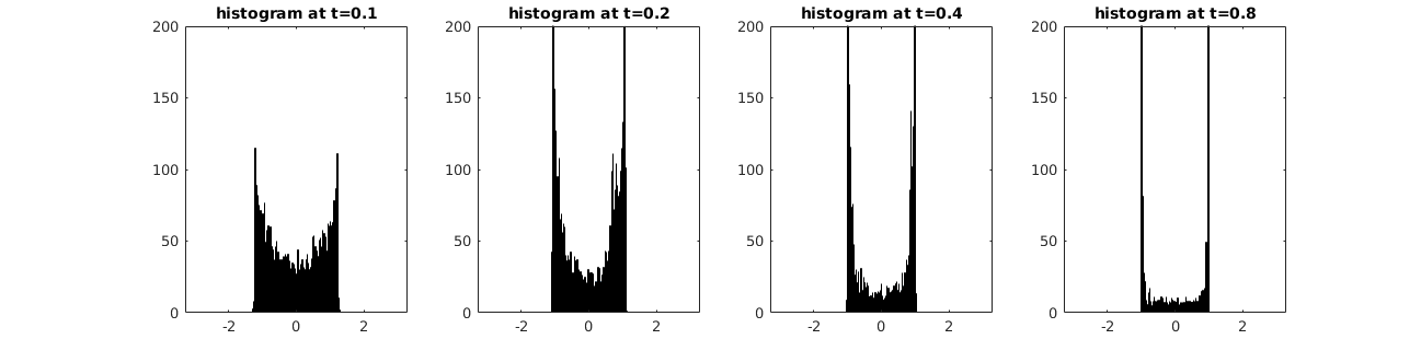 Figure 1
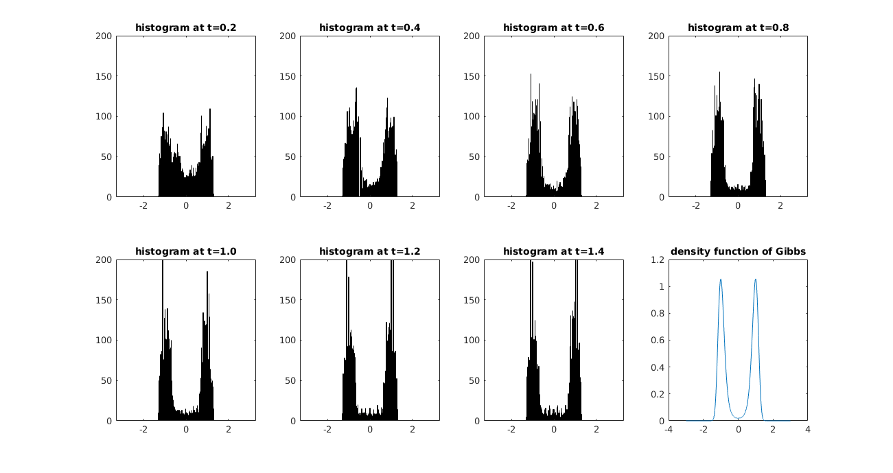 Figure 2
Peer Reviews
No public reviews on file for this paper yet. If you reviewed it on a platform where reviews are public (OpenReview, ICLR, NeurIPS, ICML), you can paste yours below so the community can read it here.
Videos
No videos yet. Explain this paper in a talk, walkthrough, or lecture? Add one.
11institutetext: University of California, Los Angeles 22institutetext: Georgia Institute of Technology
Parametric Fokker-Planck equation
Wuchen Li 11
Shu Liu 22
Hongyuan Zha 22
Haomin Zhou 22
Abstract
We derive the Fokker-Planck equation on the parametric space. It is the Wasserstein gradient flow of relative entropy on the statistical manifold. We pull back the PDE to a finite dimensional ODE on parameter space. Some analytical example and numerical examples are presented.
Keywords:
Optimal transport Information Geometry Statistical manifold Fokker-Planck equation Gradient Flow
1 Introduction
Fokker-Planck equation, a linear evolution partial differential equation (PDE), plays a crucial role in stochastic calculus, statistical physics and modeling [14, 17, 19]. Recently, people also discover its importance in statistics and machine learning [11, 16, 18]. Fokker-Planck equation describes the evolution of density functions of the stochastic process driven by a stochastic differential equation (SDE).
There is another viewpoint of Fokker-Planck equation based on optimal transport theory. It treats the equation as the gradient flow of relative entropy on probability manifold equipped with Wasserstein metric [5, 15]. Recently, the studies have been extended to information geometry [1, 2, 3], creating a new area known as Wasserstein information geometry [7, 9, 10]. Inspired by those studies, in this paper, we derive the metric tensor on parameter space by pulling back the Wasserstein metric via the parameterized pushforward map. Then we compute the Wasserstein gradient flow (an ODE system) of relative entropy defined on parameter space. This leads to a statistical manifold version of Fokker Planck equation, which can be viewed as an approximation of the original PDE.
Our work is motivated by two purposes, (1) reducing the evolution PDE to a finite dimensional ODE system on parameter space; (2) applying parameterized pushforward map to obtain an efficient sampling method to generate samples from SDE. This is different from Markov Chain Monte Carlo (MCMC) methods [12] or momentum methods [17]. In this brief presentation, we sketch the theoretical framework with illustrations on several examples. The complete results will be reported in an extended version [13].
2 Parametric Fokker-Planck equation
In this section, we briefly review the fact that Fokker-Planck equation is a Wasserstein gradient flow of relative entropy. We then introduce a Wasserstein statistical manifold generated by parameterized mapping function. Based on it, we derive the parametric Fokker-Planck equation as the gradient flow of parameterized relative entropy.
2.1 Fokker-Planck equation
Consider the Fokker-Planck equation:
[TABLE]
Here , is the divergence and gradient operator in , is the drift function and is a diffusion constant. There are several understandings for the equation (1).
On the one hand, consider the stochastic differential equation:
[TABLE]
Here is the standard Brownian motion. It is well known that the density function of stochastic process , i.e. , satisfies the Fokker-Planck equation (1).
On the other hand, equation (1) is the Wasserstein gradient flow of relative entropy. Denote the probability space supported on :
[TABLE]
Equipped with the Wasserstein metric [6, 15], is an infinite dimensional Riemmanian manifold. Denote
[TABLE]
Consider a specific and , . The Wasserstein metric tensor is defined as:
[TABLE]
where for . Here is a metric tensor, which is a positive definite bilinear form defined on tangent bundle .
The Riemannian gradient in is given as follows. Consider a smooth functional , then
[TABLE]
where is the first variation at variable . In particular, consider the relative entropy
[TABLE]
Then , and (3) forms
[TABLE]
Notice , then . The above equation is exactly Fokker-Planck equation (1).
From now on, we apply the above geometric gradient flow formulation and derive the Fokker-Planck equation (1) on parameter space.
2.2 Parameter space equipped with Wasserstein metric
We consider a parameter space as an open set in . Denote the sample space . Suppose is a pushforward map from to , which is parametrized by . For example, we can set , with ; we can also let be a neural network with parameter . We further assume that is invertible and smooth with respect to parameter and variable .
Denote as a reference probability measure with positive density defined on . For example, we can choose as the standard Gaussian. We denote as the density of .111Let be two measurable spaces, is a probability measure defined on ; let be a measurable map, then is defined as: for all measurable . We call the pushforward of measure by map . We further require: holds for all . Then for each . Denote , then .
Now the connection between and is the pushforward operation . In order to introduce the Wasserstein metric to parameter space , we assume that is an isometric immersion from to . Under this assumption, the pullback of the Wasserstein metric by is the metric tensor on . Let us denote . Then for each , is a bilinear form on , thus can be treated as an matrix. Computation of is illustrated in the following theorem:
Theorem 2.1
Suppose is isometric immersion from to . Then the metric tensor at is non-negative definite symmetric matrix and can be computed as:
[TABLE]
Or in entry-wised form:
[TABLE]
Here and is Jacobian matrix of . For each , solves the following equation:
[TABLE]
Proof
Suppose is a vector field on , for a fixed , we first compute the pushforward of at point : We choose any differentiable curve on with and . If we denote , then we have (T_{\#})_{*}\xi(\theta)=\frac{\partial\rho_{\theta_{t}}}{\partial t}\Bigr{|}_{t=0}. To compute \frac{\partial\rho_{\theta_{t}}}{\partial t}\Bigr{|}_{t=0}, we consider for any :
[TABLE]
This weak formulation reveals that
[TABLE]
Now let us compute the metric tensor . Since is isometric immersion from to , the pullback of by gives , i.e. . By definition of pullback map, for any and for any , we have:
[TABLE]
To compute the right hand side of (8), recall (2.1), we need to solve for from:
[TABLE]
[TABLE]
We can straightforwardly check that is the solution of (10). Then is computed as:
[TABLE]
Thus we can verify that:
[TABLE]
Generally speaking, the metric tensor doesn’t have an explicit form when ; but for , has an explicit form and can be computed directly.
Corollary 1
When dimension of equals 1. And we further assume that: on and . Then has an explicit form:
[TABLE]
The following theorem ensures the positive definiteness of the metric tensor :
Theorem 2.2
We follow the notations and conditions in section 2.2,2.3. Then is Riemmanian metric on iff For each , for any , we can find such that .
From now on, following [9, 10], we call Wasserstein statistical manifold.
2.3 Fokker-Planck equation on statistical manifold
Recall the relative entropy functional defined in (4), we consider . Then:
[TABLE]
As in [1], the gradient flow of on Wasserstein statistical manifold satisfies
[TABLE]
We call (13) parametric Fokker-Planck equation. The ODE (13) as the Wasserstein gradient flow on parameter space is closely related to Fokker-Planck equation on probability submanifold . We have the following theorem, which is a natural result derived from submanifold geometry:
Theorem 2.3
Suppose solves (13). Then is the gradient flow of on probability submanifold .
3 Example on Fokker-Planck equations with quadratic potential
The solution of Fokker-Planck equation on statistical manifold (13) can serve as an approximation to the solution of the original equation (1). However, in some special cases, exactly solves (1). In this section, we demonstrate such examples.
Let us consider Fokker-Planck equations with quadratic potentials whose initial conditions are Gaussian, i.e.
[TABLE]
Consider parameter space (), where is a invertible matrix with and . We define the parametric map as . We choose the reference measure . Here is the lemma we have to use:
Lemma 1
*Let be the relative entropy defined in (4) and defined in (12). For , If the vector function can be written as the linear combination of , i.e. there exists , such that . Then:
-
, which is the Wasserstein gradient of at .
-
If we denote the gradient of on as and the gradient of on the submanifold as , then .*
Proof
The detailed proof is provided in [8]. Here is an intuitive explanation: is the real vector field that moves the particles in Fokker-Planck equation; and is the approximate vector field induced by the pushforward map . If such approximate is perfect with zero error, i.e. exits such that , then and the submanifold gradient agrees with entire manifold gradient.
Now, let us come back to our example, we can compute
[TABLE]
Then we have:
[TABLE]
is affine w.r.t. .
Notice that and . We can verify that solves . By 1) of Corollary 1, . Thus ODE (13) for our example is:
[TABLE]
By 2) of Corollary 1, we know for all . This indicates that there is no local error for our approximation, one can verify that the solution to the parametric Fokker-Planck equation also solves the original equation.
In addition to previous results, we have the following corollary:
Corollary 2
The solution of Fokker-Planck equation (1) with condition(14) is Gaussian distribution for all .
Proof
If we denote as the solutions to (15),(16), set , then solves the Fokker Planck Equation (1) with conditions (14). Since the pushforward of Gaussian distribution by an affine transform is still a Gaussian, we conclude that for any , the solution is always Gaussian distribution. This is already a well known result about Fokker-Planck equation. We reprove it under our framework.
4 Numerical examples for 1D Fokker-Planck equation
Since the Wasserstein metric tensor has an explicit solution when dimension , it is convenient to numerically compute ODE (13).
For example, we can choose a series of basis functions . Each can be chosen as a sinusoidal function or a piece-wise linear function defined on a certain interval . It is also beneficial to choose orthogonal or near-orthogonal basis functions because they will keep the metric tensor far away from ill-posedness. We set 222In application, carefully choosing which is not necessarily invertibile or smooth can still provide valid results.. Then according to (11), we can compute as
[TABLE]
Recall that . The second part of is the entropy of , which can be computed by solving the following optimization problem [4]:
[TABLE]
We can solve (17) by parametrizing . Suppose the optimal solution is . Then by envelope theorem, we know can be computed as
[TABLE]
Notice that both the metric tensor and are written in forms of expectations, thus we can compute them by Monte Carlo simulations. And finally, (13) can be computed by forward Euler method.
Our numerical results are always demonstrated by sample points: For each time node , we sample points from , then are our numerical samples from distribution which solves the Fokker-Planck equation.
Here are several numerical results based on our method. We exhibit them in the form of histograms. Consider the potential . Suppose the initial distribution is . Figure 1 contains histograms of which solves at different time nodes; we know converges to as . Here is the Dirac distribution concentrated on point . Figure 2 contains histograms of which solves at different time nodes, we know will converge to Gibbs distribution , with being a normalizing constant, as . The density function of is exhibited in Figure 2.
5 Discussion
We presented a new approach for approximating Fokker-Planck equations by parameterized push-forward mapping functions. Compared to the classical moment method and MCMC method, we propose a systemic way for obtaining a finite dimensional ODE on parameter space. The ODE represents the evolution of statistical information conveyed in the original Fokker-Planck equation. In the future, we will study its geometric and statistical properties, and derive practical numerical methods for applications in scientific computing and machine learning.
Acknowledgement This project has received funding from AFOSR MURI FA9550-18-1-0502 and NSF Awards DMS–1419027, DMS-1620345, and ONR Award N000141310408.
The reference list from the paper itself. Each links out to its DOI / PubMed record.
- 1[1] S. Amari. Natural Gradient Works Efficiently in Learning. Neural Computation , 10(2):251–276, 1998.
- 2[2] S. Amari. Information Geometry and Its Applications . Number volume 194 in Applied Mathematical Sciences. Springer, Japan, 2016.
- 3[3] N. Ay, J. Jost, H. V. Lê, and L. J. Schwachhöfer. Information Geometry . Ergebnisse Der Mathematik Und Ihrer Grenzgebiete A @series of Modern Surveys in Mathematics$l 3. Folge, Volume 64. Springer, Cham, 2017.
- 4[4] M. Essid, D. Laefer, and E. G. Tabak. Adaptive Optimal Transport. ar Xiv:1807.00393 [math] , 2018.
- 5[5] R. Jordan, D. Kinderlehrer, and F. Otto. The Variational Formulation of the Fokker–Planck Equation. SIAM Journal on Mathematical Analysis , 29(1):1–17, 1998.
- 6[6] J. D. Lafferty. The Density Manifold and Configuration Space Quantization. Transactions of the American Mathematical Society , 305(2):699–741, 1988.
- 7[7] W. Li. Geometry of probability simplex via optimal transport. ar Xiv:1803.06360 [math] , 2018.
- 8[8] W. Li, S. Liu, H. Zha, and H. Zhou. Scientific computing via parametric fokker-planck equations. In preparation , 2019.