TL;DR
This paper introduces recent techniques centered around the Matrix Dyson Equation (MDE) to analyze local spectral universality in a broad class of random matrices, including those with correlated or non-identically distributed entries.
Contribution
It extends existing methods by focusing on the stability analysis of the MDE for generalized random matrices, broadening the scope of spectral universality proofs.
Findings
Stability properties of the MDE are crucial for understanding spectral behavior.
The techniques handle matrices with correlated and non-identically distributed entries.
The approach generalizes previous results on Wigner matrices.
Abstract
These lecture notes are a concise introduction of recent techniques to prove local spectral universality for a large class of random matrices. The general strategy is presented following the recent book with H.T. Yau. We extend the scope of this book by focusing on new techniques developed to deal with generalizations of Wigner matrices that allow for non-identically distributed entries and even for correlated entries. This requires to analyze a system of nonlinear equations, or more generally a nonlinear matrix equation called the Matrix Dyson Equation (MDE). We demonstrate that stability properties of the MDE play a central role in random matrix theory. The analysis of MDE is based upon joint works with J. Alt, O. Ajanki, D. Schr\"oder and T. Kr\"uger that are supported by the ERC Advanced Grant, RANMAT 338804 of the European Research Council. The lecture notes were written for the…
Click any figure to enlarge with its caption.
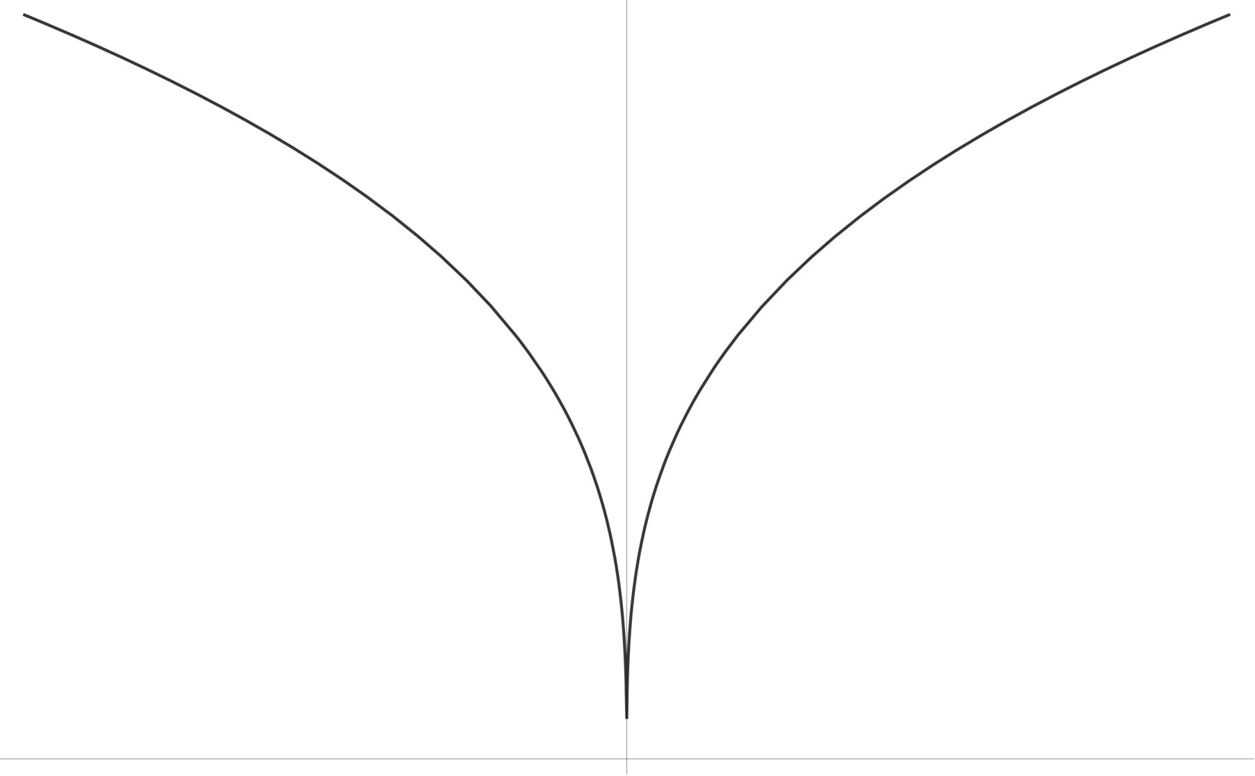 Figure 1
 Figure 2
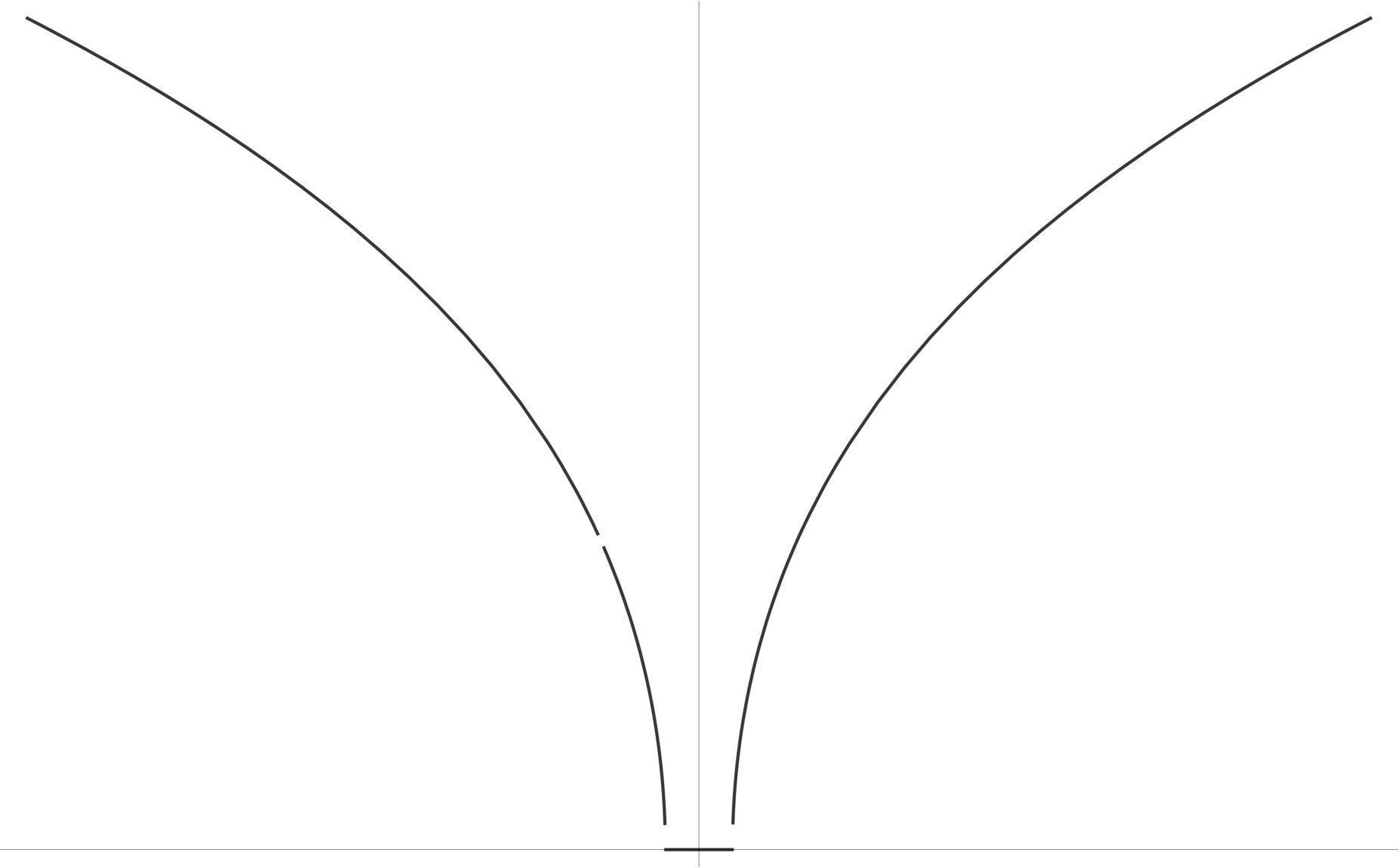 Figure 3
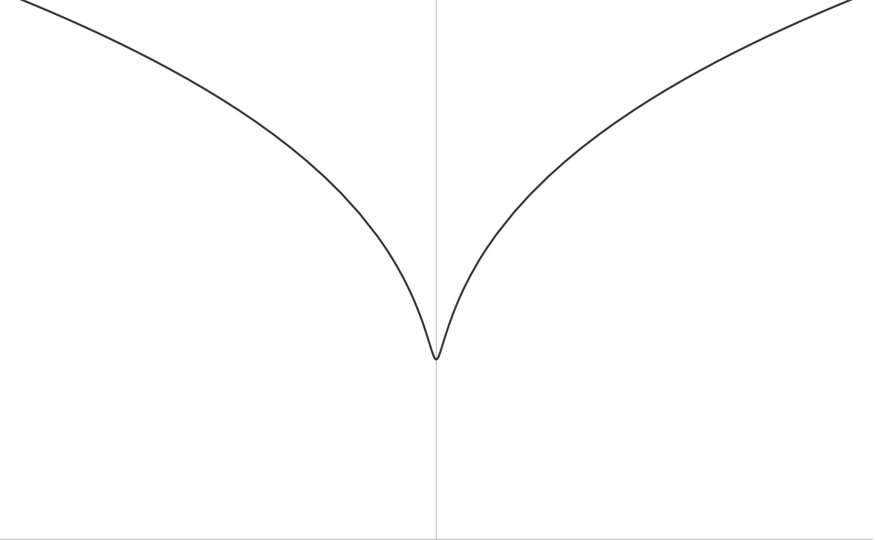 Figure 4
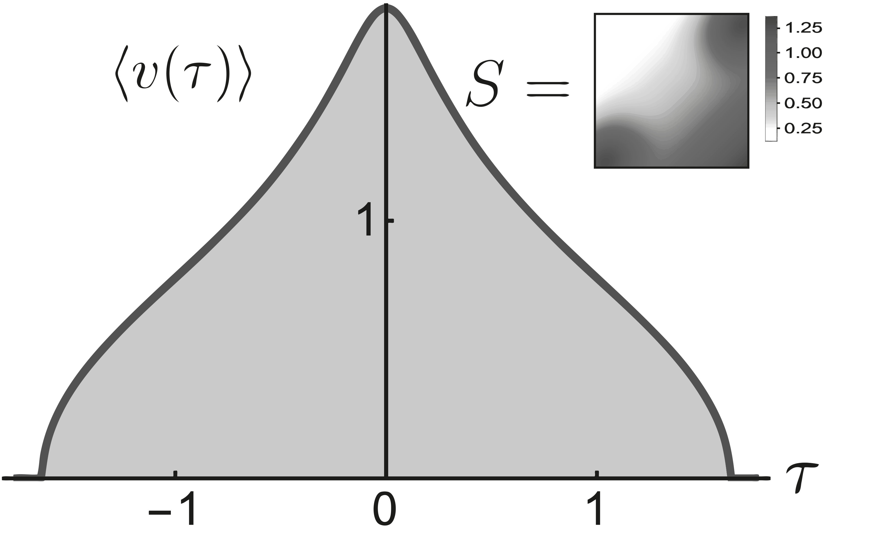 Figure 5
 Figure 6
 Figure 7
 Figure 8
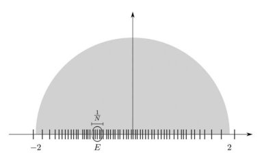 Figure 9
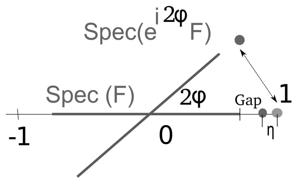 Figure 10
| Name | Dyson Equation | For | Stability op | Feature | ||||
|---|---|---|---|---|---|---|---|---|
|
|
|||||||
|
|
|||||||
|
|
|||||||
|
|
Peer Reviews
No public reviews on file for this paper yet. If you reviewed it on a platform where reviews are public (OpenReview, ICLR, NeurIPS, ICML), you can paste yours below so the community can read it here.
Code & Models
Videos
No videos yet. Explain this paper in a talk, walkthrough, or lecture? Add one.
\customizeamsrefs
The Matrix Dyson Equation
and its Applications for Random Matrices
László Erdős
Institute of Science and Technology (IST) Austria
Am Campus 1
A-3400, Klosterneuburg, Austria
(Date: Sep 1, 2017)
Abstract.
These lecture notes are a concise introduction of recent techniques to prove local spectral universality for a large class of random matrices. The general strategy is presented following the recent book with H.T. Yau [ErdYau2017]. We extend the scope of this book by focusing on new techniques developed to deal with generalizations of Wigner matrices that allow for non-identically distributed entries and even for correlated entries. This requires to analyze a system of nonlinear equations, or more generally a nonlinear matrix equation called the Matrix Dyson Equation (MDE). We demonstrate that stability properties of the MDE play a central role in random matrix theory. The analysis of MDE is based upon joint works with J. Alt, O. Ajanki, D. Schröder and T. Krüger that are supported by the ERC Advanced Grant, RANMAT 338804 of the European Research Council.
The lecture notes were written for the 27th Annual PCMI Summer Session on Random Matrices held in 2017. The current edited version will appear in the IAS/Park City Mathematics Series, Vol. 26.
Key words and phrases:
Park City Mathematics Institute, Random matrix, Matrix Dyson Equation, local semicircle law, Dyson sine kernel, Wigner-Dyson-Mehta conjecture, Tracy-Widom distribution, Dyson Brownian motion
2010 Mathematics Subject Classification:
Primary 15B52; Secondary 82B44
Partially supported by ERC Advanced Grant, RANMAT 338804
Contents
-
1.2.3 Eigenvalues on microscopic scales: universality of local eigenvalue statistics
-
2.3 The semicircle law for Wigner matrices via the moment method
-
5.2 The “grand” universality conjecture for disordered quantum systems
-
6.2 Local laws for Wigner-type and correlated random matrices
-
6.3 Bulk universality and other consequences of the local law
1. Introduction
*“Perhaps I am now too courageous when I try to guess the distribution of the distances between successive levels (of energies of heavy nuclei). Theoretically, the situation is quite simple if one attacks the problem in a simpleminded fashion. The question is simply what are the distances of the characteristic values of a symmetric matrix with random coefficients.” *
Eugene Wigner on the Wigner surmise, 1956
The cornerstone of probability theory is the fact that the collective behavior of many independent random variables exhibits universal patterns; the obvious examples are the law of large numbers (LLN) and the central limit theorem (CLT). They assert that the normalized sum of independent, identically distributed (i.i.d.) random variables converge to their common expectation value:
[TABLE]
as , and their centered average with a normalization converges to the centered Gaussian distribution with variance :
[TABLE]
The convergence in the latter case is understood in distribution, i.e. tested against any bounded continuous function :
[TABLE]
where is an distributed normal random variable.
These basic results directly extend to random vectors instead of scalar valued random variables. The main question is: what are their analogues in the non-commutative setting, e.g. for matrices? Focusing on their spectrum, what do eigenvalues of typical large random matrices look like? Is there a deterministic limit of some relevant random quantity, like the average in case of the LLN (1.0.1). Is there some stochastic universality pattern arising, similarly to the ubiquity of the Gaussian distribution in Nature owing to the central limit theorem?
These natural questions could have been raised from pure curiosity by mathematicians, but historically random matrices first appeared in statistics (Wishart in 1928 [Wis1928]), where empirical covariance matrices of measured data (samples) naturally form a random matrix ensemble and the eigenvalues play a crucial role in principal component analysis. The question regarding the universality of eigenvalue statistics, however, appeared only in the 1950’s in the pioneering work [Wig1955] of Eugene Wigner. He was motivated by a simple observation looking at data from nuclear physics, but he immediately realized a very general phenomenon in the background. He noticed from experimental data that gaps in energy levels of large nuclei tend to follow the same statistics irrespective of the material. Quantum mechanics predicts that energy levels are eigenvalues of a self-adjoint operator, but the correct Hamiltonian operator describing nuclear forces was not known at that time. Instead of pursuing a direct solution of this problem, Wigner appealed to a phenomenological model to explain his observation. His pioneering idea was to model the complex Hamiltonian by a random matrix with independent entries. All physical details of the system were ignored except one, the symmetry type: systems with time reversal symmetry were modeled by real symmetric random matrices, while complex Hermitian random matrices were used for systems without time reversal symmetry (e.g. with magnetic forces). This simple-minded model amazingly reproduced the correct gap statistics. Eigenvalue gaps carry basic information about possible excitations of the quantum systems. In fact, beyond nuclear physics, random matrices enjoyed a renaissance in the theory of disordered quantum systems, where the spectrum of a non-interacting electron in a random impure environment was studied. It turned out that eigenvalue statistics is one of the basic signatures of the celebrated metal-insulator, or Anderson transition in condensed matter physics [And1958].
1.1. Random matrix ensembles
Throughout these notes we will consider square matrices of the form
[TABLE]
The entries are real or complex random variables constrained by the symmetry
[TABLE]
so that is either Hermitian (complex) or symmetric (real). In particular, the eigenvalues of , are real and we will be interested in their statistical behavior induced by the randomness of as the size of the matrix goes to infinity. Hermitian symmetry is very natural from the point of view of physics applications and it makes the problem much more tractable mathematically. Nevertheless, there has recently been an increasing interest in non-hermitian random matrices as well motivated by systems of ordinary differential equations with random coefficients arising in biological networks (see, e.g. [EKR, Nelson2016] and references therein).
There are essentially two customary ways to define a probability measure on the space of random matrices that we now briefly introduce. The main point is that either one specifies the distribution of the matrix elements directly or one aims at a basis-independent measure. The prototype of the first case is the Wigner ensembles and we will be focusing on its natural generalizations in these notes. The typical example of the second case are the invariant ensembles. We will briefly introduce them now.
1.1.1. Wigner ensemble
The most prominent example of the first class is the traditional Wigner matrix, where the matrix elements are i.i.d. random variables subject to the symmetry constraint . More precisely, Wigner matrices are defined by assuming that
[TABLE]
In the real symmetric case, the collection of random variables are independent, identically distributed, while in the complex hermitian case the distributions of and are independent and identical.
The common variance of the matrix elements is the single parameter of the model; by a trivial rescaling we may fix it conveniently. The normalization chosen in (1.1.2) guarantees that the typical size of the eigenvalues remain of order 1 even as tends to infinity. To see this, we may compute the expectation of the trace of in two different ways:
[TABLE]
indicating that on average. In fact, much stronger bounds hold and one can prove that
[TABLE]
in probability.
In these notes we will focus on Wigner ensembles and their extensions, where we will drop the condition of identical distribution and we will weaken the independence condition. We will call them Wigner type and correlated ensembles. Nevertheless, for completeness we also present the other class of random matrices.
1.1.2. Invariant ensembles
The ensembles in the second class are defined by the measure
[TABLE]
Here is the flat Lebesgue measure on (in case of complex Hermitian matrices and , is the Lebesgue measure on the complex plane instead of ). The (potential) function is assumed to grow mildly at infinity (some logarithmic growth would suffice) to ensure that the measure defined in (1.1.4) is finite. The parameter distinguishes between the two symmetry classes: for the real symmetric case, while for the complex hermitian case – for traditional reason we factor this parameter out of the potential.
Finally, is the normalization factor to make a probability measure. Similarly to the normalization of the variance in (1.1.2), the factor in the exponent in (1.1.4) guarantees that the eigenvalues remain order one even as . This scaling also guarantees that empirical density of the eigenvalues will have a deterministic limit without further rescaling.
Probability distributions of the form (1.1.4) are called invariant ensembles since they are invariant under the orthogonal or unitary conjugation (in case of symmetric or Hermitian matrices, respectively). For example, in the Hermitian case, for any fixed unitary matrix , the transformation
[TABLE]
leaves the distribution (1.1.4) invariant thanks to and that .
An important special case is when is a quadratic polynomial, after shift and rescaling we may assume that . In this case
[TABLE]
i.e. the measure factorizes and it is equivalent to independent Gaussians for the matrix elements. The factor in the definition (1.1.4) and the choice of ensure that we recover the normalization (1.1.2). (A pedantic reader may notice that the normalization of the diagonal element for the real symmetric case is off by a factor of 2, but this small discrepancy plays no role.) The invariant Gaussian ensembles, i.e. (1.1.4) with , are called Gaussian orthogonal ensemble (GOE) for the real symmetric case and Gaussian unitary ensemble (GUE) for the complex hermitian case .
Wigner matrices and invariant ensembles form two different universes with quite different mathematical tools available for their studies. In fact, these two classes are almost disjoint because the Gaussian ensembles are the only invariant Wigner matrices. This is the content of the following lemma:
Lemma 1.1.5** ([Dei1999] or Theorem 2.6.3 [Meh1991]).**
Suppose that the real symmetric or complex Hermitian matrix ensembles given in (1.1.4) have independent entries , . Then is a quadratic polynomial, with . This means that apart from a trivial shift and normalization, the ensemble is GOE or GUE.
The significance of the Gaussian ensembles is that they allow for explicit calculations that are not available for Wigner matrices with general non-Gaussian single entry distribution. In particular the celebrated Wigner-Dyson-Mehta correlation functions can be explicitly obtained for the GOE and GUE ensembles. Thus the typical proof of identifying the eigenvalue correlation function for a general matrix ensemble goes through universality: one first proves that the correlation function is independent of the distribution, hence it is the same as GUE/GOE, and then, in the second step, one computes the GUE/GOE correlation functions. This second step has been completed by Gaudin, Mehta and Dyson in the 60’s by an ingenious calculation, see e.g. the classical treatise by Mehta [Meh1991].
One of the key ingredients of the explicit calculations is the surprising fact that the joint (symmetrized) density function of the eigenvalues, can be computed explicitly for any invariant ensemble. It is given by
[TABLE]
where the constant ensures the normalization, but its exact value is typically unimportant.
Remark 1.1.7*.*
In other sections of these notes we usually label the eigenvalues in increasing order so that their probability density, denoted by \widetilde{p}_{N}(\mbox{\boldmath\lambda}), is defined on the set
[TABLE]
For the purpose of (1.1.6), however, we dropped this restriction and we consider to be a symmetric function of variables, \mbox{\boldmath\lambda}=(\lambda_{1},\ldots,\lambda_{N}) on . The relation between the ordered and unordered densities is clearly \widetilde{p}_{N}(\mbox{\boldmath\lambda})=N!\,p_{N}(\mbox{\boldmath\lambda})\cdot{\bf 1}(\mbox{\boldmath\lambda}\in\Xi^{(N)}).
The emergence of the Vandermonde determinant in (1.1.6) is a result of integrating out the “angle” variables in (1.1.4), i.e., the unitary matrix in the diagonalization of . This is a remarkable formula since it gives a direct access to the eigenvalue distribution. In particular, it shows that the eigenvalues are strongly correlated. For example, no two eigenvalues can be too close to each other since the corresponding probability is suppressed by the factor for any ; this phenomenon is called the level repulsion. We remark that level repulsion also holds for Wigner matrices with smooth distribution [ErdSchYau2010] but its proof is much more involved.
In fact, one may view the ensemble (1.1.6) as a statistical physics question by rewriting as a classical Gibbs measure of a point particles on the line with a logarithmic mean field interaction:
[TABLE]
with a Hamiltonian
[TABLE]
This ensemble of point particles with logarithmic interactions is also called log-gas. We remark that viewing the Gibbs measure (1.1.8) as the starting point and forgetting about the matrix ensemble behind, the parameter does not have to be 1 or 2; it can be any positive number, , and it has the interpretation of the inverse temperature. We will not pursue general invariant ensembles in these notes.
1.2. Eigenvalue statistics on different scales
The normalization both in (1.1.2) and (1.1.4) is chosen in such a way that the typical eigenvalues remain of order 1 even in the large limit. In particular, the typical distance between neighboring eigenvalues is of order . We distinguish two different scales for studying eigenvalues: macroscopic and microscopic scales. With our scaling, the macroscopic scale is order one and on this scale we detect the cumulative effect of eigenvalues with some positive constant . In contrast, on the microscopic scales individual eigenvalues are detected; this scale is typically of order . However, near the spectral edges, where the density of eigenvalues goes to zero, the typical eigenvalue spacing hence the microscopic scale may be larger. Some phenomena (e.g. fluctuations of linear statistics of eigenvalues) occur on various mesoscopic scales that lie between the macroscopic and the microscopic scales.
1.2.1. Eigenvalue density on macroscopic scales: global laws
The first and simplest question is to determine the eigenvalue density, i.e. the behavior of the empirical eigenvalue density or empirical density of states
[TABLE]
in the large limit. This is a random measure, but under very general conditions it converges to a deterministic measure, similarly to self-averaging property encoded in the law of large numbers (1.0.1).
For Wigner ensemble, the empirical distribution of eigenvalues converges to the Wigner semicircle law. To formulate it more precisely, note that the typical spacing between neighboring eigenvalues is of order , so in a fixed interval , one expects macroscopically many (of order ) eigenvalues. More precisely, it can be shown (first proof was given by Wigner [Wig1955]) that for any fixed real numbers,
[TABLE]
where denotes the positive part of the number . Alternatively, one may formulate the Wigner semicircle law as the weak convergence in probability of the empirical distribution to the semicircle distribution, . This means that the limit
[TABLE]
holds in probability for any bounded continuous function , i.e.,
[TABLE]
for any as .
Note that the emergence of the semicircle density is already a certain form of universality: the common distribution of the individual matrix elements is “forgotten”; the density of eigenvalues is asymptotically always the same, independently of the details of the distribution of the matrix elements.
We will see that for a more general class of Wigner type matrices with zero expectation but not identical distribution a similar limit statement holds for the empirical density of eigenvalues, i.e. there is a deterministic density function such that
[TABLE]
holds. The density function thus approximates the empirical density, so we will call it asymptotic density (of states). In general it is not the semicircle density, but is determined by the second moments of the matrix elements and it is independent of other details of the distribution. For independent entries, the variance matrix
[TABLE]
contains all necessary information. For matrices with correlated entries, all relevant second moments are encoded in the linear operator
[TABLE]
acting on matrices. It is one of the key questions in random matrix theory to compute the asymptotic density from the second moments; we will see that the answer requires solving a system of nonlinear equations, that will be commonly called the Dyson equation. The explicit solution leading to the semicircle law is available only for Wigner matrices, or a little bit more generally, for ensembles with the property
[TABLE]
These are called generalized Wigner ensembles and have been introduced in [EYY].
For invariant ensembles, the self-consistent density depends on the potential function . It can be computed by solving a convex minimization problem, namely it is the the unique minimizer of the functional
[TABLE]
In both cases, under some mild conditions on the variances or on the potential , respectively, the asymptotic density is compactly supported.
1.2.2. Eigenvalues on mesoscopic scales: local laws
The Wigner semicircle law in the form (1.2.2) asymptotically determines the number of eigenvalues in a fixed interval . The number of eigenvalues in such intervals is comparable with . However, keeping in mind the analogy with the law of large numbers, it is natural to raise the question whether the same asymptotic relation holds if the length of the interval shrinks to zero as . To expect a deterministic answer, the interval should still contain many eigenvalues, but this would be guaranteed by . This turns out to be correct and the local semicircle law asserts that
[TABLE]
uniformly in as long as for any and is not at the edge, . Here we considered the interval , i.e. we fixed its center and viewed its length as an -dependent parameter. (The factors can be improved to some -power.)
1.2.3. Eigenvalues on microscopic scales: universality of local eigenvalue statistics
Wigner’s original observation concerned the distribution of the distances between consecutive (ordered) eigenvalues, or gaps. In the bulk of the spectrum, i.e. in the vicinity of a fixed energy level with in case of the semicircle law, the gaps have a typical size of order (at the spectral edge, , the relevant microscopic scale is of order , but we will not pursue edge behavior in these notes). Thus the corresponding rescaled gaps have the form
[TABLE]
where is the asymptotic density, e.g. for Wigner matrices. Wigner predicted that the fluctuations of the gaps are universal and their distribution is given by a new law, the Wigner surmise. Thus there exists a random variable , depending only on the symmetry class , such that
[TABLE]
in distribution, for any gap away from the edges, i.e., if with some fixed .
This might be viewed as the random matrix analogue of the central limit theorem. Note that universality is twofold. First, the distribution of is independent of the index (as long as is away from the edges). Second, more importantly, the limiting gap distribution is independent of the distribution of the matrix elements, similarly to the universal character of the central limit theorem.
However, the gap universality holds much more generally than the semicircle law: the rescaled gaps (1.2.7) follow the same distribution as the gaps of the GUE or GOE (depending on the symmetry class) essentially for any random matrix ensemble with “sufficient” amount of randomness. In particular, it holds for invariant ensembles, as well as for Wigner type and correlated random matrices, i.e. for very broad extensions of the original Wigner ensemble. In fact, it holds much beyond the traditional realm of random matrices; it is conjectured to hold for any random matrix describing a disordered quantum system in the delocalized regime, see Section 5.2 later.
The universality on microscopic scales can also be expressed in terms of the appropriately rescaled correlation functions. In fact, in this way the formulas are more explicit. First we define the correlation functions.
Definition 1.2.8**.**
Let be the joint symmetrized probability distribution of the eigenvalues. For any , the -point correlation function is defined by
[TABLE]
The significance of the correlation functions is that with their help one can compute the expectation value of any symmetrized observable. For example, for any bounded continuous test function of two variables we have, directly from the definition of the correlation functions, that
[TABLE]
where the expectation is w.r.t. the probability density or in this case w.r.t. the original random matrix ensemble. Similar formula holds for observables of any number of variables. In particular, the global law (1.2.3) implies that the one point correlation function converges to the asymptotic density
[TABLE]
weakly, since
[TABLE]
Correlation functions are difficult to compute in general, even if the joint density function is explicitly given as in the case of the invariant ensembles (1.1.6). Naively one may think that computing the correlation functions in this latter case boils down to an elementary calculus exercise by integrating out all but a few variables. However, that task is complicated.
As mentioned, one may view the joint density of eigenvalues of invariant ensembles (1.1.6) as a Gibbs measure of a log-gas and here can be any positive number (inverse temperature). The universality of correlation functions is a valid question for all -log-gases that has been positively answered in [BouErdYau2014, BouErdYau2012, BouErdYau2014-2, BekFigGui2015, Shc2014] by showing that for a sufficiently smooth potential (in fact suffices) the correlation functions depend only on and are independent of . We will not pursue general invariant ensembles in these notes.
The logarithmic interaction is of long range, so the system (1.1.8) is strongly correlated and standard methods of statistical mechanics to compute correlation functions cannot be applied. The computation is quite involved even for the simplest Gaussian case, and it relies on sophisticated identities involving Hermite orthogonal polynomials. These calculations have been developed by Gaudin, Mehta and Dyson in the 60’s and can be found, e.g. in Mehta’s book [Meh1991]. Here we just present the result for the most relevant cases.
We fix an energy in the bulk, i.e., , and we rescale the correlation functions by a factor around to make the typical distance between neighboring eigenvalues 1. These rescaled correlation functions then have a universal limit:
Theorem 1.2.11**.**
For GUE ensembles, the rescaled correlation functions converge to the determinantal formula with the sine kernel, , i.e.
[TABLE]
as weak convergence of functions in the variables .
Formula (1.2.12) holds for the GUE case. The corresponding expression for GOE is more involved [Meh1991, AndGuiZei2010]
[TABLE]
Here the determinant is understood as the trace of the quaternion determinant after the canonical correspondence between quaternions , , and complex matrices given by
[TABLE]
Note that the limit in (1.2.12) is universal in the sense that it is independent of the energy . However, universality also holds in a much stronger sense, namely that the local statistics (limits of rescaled correlation functions) depend only on the symmetry class, i.e. on , and are independent of any other details. In particular, they are always given by the sine kernel (1.2.12) or (1.2.13) not only for the Gaussian case but for any Wigner matrices with arbitrary distribution of the matrix elements, as well as for any invariant ensembles with arbitrary potential . This is the Wigner-Dyson-Mehta (WDM) universality conjecture, formulated precisely in Mehta’s book [Meh1991] in the late 60’s.
The WDM conjecture for invariant ensembles has been in the focus of very intensive research on orthogonal polynomials with general weight function (the Hermite polynomials arising in the Gaussian setup have Gaussian weight function). It motivated the development of the Riemann-Hilbert method [FokItcKit1992], that was originally brought into this subject by Fokas, Its and Kitaev [FokItcKit1992], and the universality of eigenvalue statistics was established for large classes of invariant ensembles by Bleher-Its [BleIts1999] and by Deift and collaborators [Dei1999, DeiGio2007-2, DeiKriMcLVen1999]. The key element of this success was that invariant ensembles, unlike Wigner matrices, have explicit formulas (1.1.6) for the joint densities of the eigenvalues. With the help of the Vandermonde structure of these formulas, one may express the eigenvalue correlation functions as determinants whose entries are given by functions of orthogonal polynomials.
For Wigner ensembles, there are no explicit formulas for the joint density of eigenvalues or for the correlation functions statistics and the WDM conjecture was open for almost fifty years with virtually no progress. The first significant advance in this direction was made by Johansson [Joh2001], who proved the universality for complex Hermitian matrices under the assumption that the common distribution of the matrix entries has a substantial Gaussian component, i.e., the random matrix is of the form where is a general Wigner matrix, is the GUE matrix, and is a certain, not too small, positive constant independent of . His proof relied on an explicit formula by Brézin and Hikami [BreHik1996, BreHik1997] that uses a certain version of the Harish-Chandra-Itzykson-Zuber formula [ItzZub1980]. These formulas are available for the complex Hermitian case only, which restricted the method to this symmetry class.
Exercise 1.2.14**.**
Verify formula (1.2.10).
1.2.4. The three step strategy
The WDM conjecture in full generality has recently been resolved by a new approach called the three step strategy that has been developed in a series of papers by Erdős, Schlein, Yau and Yin between 2008 and 2013 with a parallel development by Tao and Vu. A detailed presentation of this method can be found in [ErdYau2017], while a shorter summary was presented in [ErdYau2012-2].
This approach consists of the following three steps:
Step 1. Local semicircle law: It provides an a priori estimate showing that the density of eigenvalues of generalized Wigner matrices is given by the semicircle law at very small microscopic scales, i.e., down to spectral intervals that contain eigenvalues.
Step 2. Universality for Gaussian divisible ensembles: It proves that the local statistics of Gaussian divisible ensembles are the same as those of the Gaussian ensembles as long as , i.e., already for very small .
Step 3. Approximation by a Gaussian divisible ensemble: It is a type of “density argument” that extends the local spectral universality from Gaussian divisible ensembles to all Wigner ensembles.
The conceptually novel point is Step 2. The eigenvalue distributions of the Gaussian divisible ensembles, written in the form , are the same as that of the solution of a *matrix valued Ornstein-Uhlenbeck (OU) process *
[TABLE]
for any time , where is a matrix valued standard Brownian motion of the corresponding symmetry class (The OU process is preferable over its rescaled version since it keeps the variance constant). Dyson [Dys1962] observed half a century ago that the dynamics of the eigenvalues of is given by an interacting stochastic particle system, called the Dyson Brownian motion (DBM), where the eigenvalues are the particles:
[TABLE]
Here are independent white noises.
In addition, the invariant measure of this dynamics is exactly the eigenvalue distribution of GOE or GUE, i.e. (1.1.6) with . This invariant measure is thus a Gibbs measure of point particles in one dimension interacting via a long range logarithmic potential. In fact, can be any positive parameter, the corresponding DBM (1.2.16) may be studied even if there is no invariant matrix ensemble behind. Using a heuristic physical argument, Dyson remarked [Dys1962] that the DBM reaches its “local equilibrium” on a short time scale . We call this Dyson’s conjecture, although it was rather an intuitive physical picture than an exact mathematical statement. Step 2 gives a precise mathematical meaning of this vague idea. The key point is that by applying local relaxation to all initial states (within a reasonable class) simultaneously, Step 2 generates a large set of random matrix ensembles for which universality holds. For the purpose of universality, this set is sufficiently dense so that any Wigner matrix is sufficiently close to a Gaussian divisible ensemble of the form with a suitably chosen .
We note that in the Hermitian case, Step 2 can be circumvented by using the Harish-Chandra-Itzykson-Zuber formula. This approach was followed by Tao and Vu [TaoVu2011] who gave an alternative proof of universality for Wigner matrices in the Hermitian symmetry class as well as for the real symmetric class but only under a certain moment matching condition.
The three step strategy has been refined and streamlined in the last years. By now it has reached a stage when the content of Step 2 and Step 3 can be presented as a very general “black-box” result that is model independent assuming that Step 1, the local law, holds. The only model dependent ingredient is the local law. Hence to prove local spectral universality for a new ensemble, one needs to verify the local law. Thus in these lecture notes we will focus on the recent developments in the direction of the local laws.
We will discuss generalizations of the original Wigner ensemble to relax the basic conditions “independent, identically distributed”. First we drop the identical distribution and allow the variances to vary. The simplest class is the generalized Wigner matrices, defined in (1.2.5), which still leads to the Wigner semicircle law. The next level of generality is to allow arbitrary matrix of variances . The density of states is not the semicircle any more and we need to solve a genuine vector Dyson equation to find the answer. The most general case discussed in these notes are correlated matrices, where different matrix elements have nontrivial correlation that leads to a matrix Dyson equation. In all cases we keep the mean field assumption, i.e. the typical size of the matrix elements is . Since Wigner’s vision on the universality of local eigenvalue statistics predicts the same universal behavior for a much larger class of hermitian random matrices (or operators), it is fundamentally important to extend the validity of the mathematical proofs as much as possible beyond the Wigner case.
We remark that there are several other directions to extend the Wigner ensemble that we will not discuss here in details, we just mention some of them with a few references, but we do not aim at completeness; apologies for any omissions. First, in these notes we will assume very high moment conditions on the matrix elements. These make the proofs easier and the tail probabilities of the estimates stronger. Several works have focused on lowering the moment assumption [Joh2012, GotNauTik2015, Aggarwal2016] and even considering heavy tailed distributions [BenPech2014, BorGui02016]. An important special case is the class of sparse matrices such as adjacency matrix of Erdős-Rényi random graphs and -regular graphs [ErdKnoYauYin2013-2, ErdKnoYauYin2012, BauHuaKnoYau2015, HuaLanYau2015, BauKnoYau2015]. Another direction is to remove the condition that the matrix elements are centered; this ensemble often goes under the name of deformed Wigner matrices. One typically separates the expectation and writes , where is a deterministic matrix and is a Wigner matrix with centered entries. Diagonal deformations ( is diagonal) are easier to handle, this class was considered even for a large diagonal in [ORourkeVu2014, KnoYin2013, KnoYin2014, LeeSchSteYau2016]. The general was considered in [HeKnowlesRosenthal2016]. Finally, a very challenging direction is to depart from the mean field condition, i.e. allow some matrix elements to be much bigger than . The ultimate example is the random band matrices that goes towards the random Schrödinger operators [Sch2009, Sod2010, ErdKno2011, ErdKnoYauYin2013, ErdKnoYau2013, TShc2014, TShc2014-2, Shc2015, BaoErd2016].
1.2.5. User’s guide
These lecture notes were intended to Ph.D students and postdocs with general interest in analysis and probability; we assume knowledge of these areas on a beginning Ph.D. level. The overall style is informal, the proof of many statements are only sketched or indicated. Several technicalities are swept under the rug – for the precise theorems the reader should consult with the original papers. We emphasise conveying the main ideas in a colloquial way.
In Section 2 we collected basic tools from analysis such as Stieltjes transform and resolvent. We also introduce the semicircle law. We outline the moment method that was traditionally important in random matrices, but we will not rely on it in these notes, so this part can be skipped. In Section 3 we outline the main method to obtain local laws, the resolvent approach and we explain in an informal way its two constituents; the probabilistic and deterministic parts. In Section 4 we introduce four models of Wigner-like ensembles with increasing complexity and we informally explain the novelty and the additional complications for each model. Section 5 on the physical motivations to study these models is a detour. Readers interested only in the mathematical aspects may skip this section. Section 6 contains our main results on the local law formulated in a mathematically precise form. We did not aim at presenting the strongest results and the weakest possible conditions; the selection was guided to highlight some key phenomena. Some consequences of these local laws are also presented with sketchy proofs. Section 7 and 8 contain the main mathematical part of these notes, here we give a more detailed analysis of the vector and the matrix Dyson equation and their stability properties. In these sections we aim at rigorous presentation although not every proof contains all details. Finally, in Section 9 we present the main ideas of the proof of the local laws based on stability results on the Dyson equation.
These lecture notes are far from being a comprehensive text on random matrices. Many key issues are left out and even those we discuss will be presented in their simplest form. For more interested readers, we refer to the recent book [ErdYau2017] that focuses on the three step strategy and discusses all steps in details. For readers interested in other aspects of random matrix theory, in addition to the classical book of Mehta [Meh1991], several excellent works are available that present random matrices in a broader scope. The books by Anderson, Guionnet and Zeitouni [AndGuiZei2010] and Pastur and Shcherbina [PasShc2011] contain extensive material starting from the basics. Tao’s book [Tao2012] provides a different aspect to this subject and is self-contained as a graduate textbook. Forrester’s monograph [For2010] is a handbook for any explicit formulas related to random matrices. Finally, [AkeBaiDi-2011] is an excellent comprehensive overview of diverse applications of random matrix theory in mathematics, physics, neural networks and engineering.
Notational conventions. In order to focus on the essentials, we will not follow the dependence of various constants on different parameters. In particular, we will use the generic letters and to denote positive constants, whose values may change from line to line and which may depend on some fixed basic parameters of the model. For two positive quantities and , we will write to indicate that there exists a constant such that . If and are comparable in the sense that and , then we write . In informal explanations, we will often use which indicates closeness in a not precisely specified sense. We introduce the notation for the set of integers between any two real numbers . We will usually denote vectors in by boldface letters; .
*Acknowledgement. * A special thank goes to Torben Krüger for many discussions and suggestions on the presentation of this material as well as for his careful proofreading and invaluable comments. I am also very grateful to both referees for many constructive suggestions, as well as to Ian Morrison for the excellent editing work.
2. Tools
2.1. Stieltjes transform
In this section we introduce our basic tool, the Stieltjes transform of a measure. We denote the open upper half of the complex plane by
[TABLE]
Definition 2.1.1**.**
Let be a Borel probability measure on . Its Stiltjes transform at a spectral parameter is defined by
[TABLE]
Exercise 2.1.3**.**
The following three properties are straightforward to check:
- i)
The Stieltjes transform is analytic on and it maps to , i.e. .
- ii)
We have as .
- iii)
We have the bound
[TABLE]
In fact, properties i)-ii) characterize the Stieltjes transform in a sense that if a function satisfies i)–ii), then there exists a probability measure such that (for the proof, see e.g. Appendix B of [Weidmann]; it is also called the Nevanlinna’s representation theorem).
From the Stieltjes transform one may recover the measure:
Lemma 2.1.4** (Inverse Stieltjes transform).**
Suppose that is a probability measure on and let be its Stieltjes transform. Then for any we have
[TABLE]
Furthermore, if is absolutely continuous with respect to the Lebesgue measure, i.e. with some density function , then
[TABLE]
pointwise for almost every .
In particular, Lemma 2.1.4 guarantees that if and only of , i.e. the Stieltjes transform uniquely characterizes the measure. Furthermore, pointwise convergence of a sequence of Stieltjes transforms is equivalent to weak convergence of the measures. More precisely, we have
Lemma 2.1.5**.**
Let be a sequence of probability measures and let be their Stieltjes transforms. Suppose that
[TABLE]
exists for any and satisfies property ii), i.e. as . Then there exists a probability measure such that and converges to in distribution.
The proof can be found e.g. in [GeronimoHill] and it relies on Lemma 2.1.4 and Montel’s theorem. The converse of Lemma 2.1.5 is trivial: if the sequence converges in distribution to a probability measure , then clearly pointwise, since the Stieltjes transform for any fixed is just the integral of the continuous bounded function . Note that the additional condition ii) is a compactness (tightness) condition, it prevents that part of the measures escape to infinity in the limit.
All these results are very similar to the Fourier transform (characteristic function)
[TABLE]
of a probability measure. In fact, there is a direct connection between them;
[TABLE]
for any and . In particular, due to the regularizing factor , the large behavior of the Fourier transform is closely related to the small behavior of the Stieltjes transform.
Especially important is the imaginary part of the Stieltjes transform since
[TABLE]
which can also be viewed as the convolution of with the Cauchy kernel on scale :
[TABLE]
indeed
[TABLE]
Up to a normalization , the Cauchy kernel is an approximate delta function on scale . Clearly
[TABLE]
and the overwhelming majority of its mass is supported on scale :
[TABLE]
for any . Due to standard properties of the convolution, the moral of the story is that ** resolves the measure on a scale around an energy **.
Notice that the small regime is critical; it is the regime where the integral in the definition of the Stieltjes transform (2.1.2) becomes more singular, and properties of the integral more and more depend on the local smoothness properties of the measure. In general, the regularity of the measure on some scales is directly related to the Stieltjes transform with .
The Fourier transform of for large also characterizes the local behavior of the measure on scales , We will nevertheless work with the Stieltjes transform since for hermitian matrices (or self-adjoint operators in general) it is directly related to the resolvent, it is relatively easy to handle and it has many convenient properties.
Exercise 2.1.6**.**
Prove Lemma 2.1.4 by using Fubini’s theorem and Lebesgue density theorem.
2.2. Resolvent
Let be a hermitian matrix, then its resolvent at spectral parameter is defined as
[TABLE]
In these notes, the spectral parameter will always be in the upper half plane, . We usually follow the convention that , where will often be referred as “energy” alluding to the quantum mechanical interpretation of .
Let be the normalized empirical measure of the eigenvalues of :
[TABLE]
Then clearly the normalized trace of the resolvent is
[TABLE]
exactly the Stieltjes transform of the empirical measure. This relation justifies why we focus on the Stieltjes transform; based upon Lemma 2.1.5, if we could identify the (pointwise) limit of , then the asymptotic eigenvalue density would be given by the inverse Stieltjes transform of the limit.
Since is a discrete (atomic) measure on small scales, it may behave very badly (i.e. it is strongly fluctuating and may blow up) for smaller than , depending on whether there happens to be an eigenvalue in an -vicinity of . Since the eigenvalue spacing is (typically) of order , for there is no approximately deterministic (“self-averaging”) behavior of . However, as long as , we may hope a law of large number phenomenon; this would be equivalent to the fact that the eigenvalue density does not have much fluctuation above its inter-particle scale . The local law on down to the smallest possible (optimal) scale will confirm this hope.
In fact, the resolvent carries much more information than merely its trace. In general the resolvent of a hermitian matrix is a very rich object: it gives information on the eigenvalues and eigenvectors for energies near the real part of the spectral parameter. For example, by spectral decomposition we have
[TABLE]
where are the (-normalized) eigenvectors associated with . (Here we used the Dirac notation for the orthogonal projection to the one-dimensional space spanned by .) For example, the diagonal matrix elements of the resolvent at are closely related to the eigenvectors with eigenvalues near :
[TABLE]
Notice that for very small , the factor effectively reduces the sum from all to those indices where is -close to ; indeed this factor changes from the very large value to a very small value as moves away. Roughly speaking
[TABLE]
This idea can be made rigorous at least as an upper bound on each summand. A physically important consequence will be that one may directly obtain bounds on the eigenvectors: for any fixed we have
[TABLE]
In other words, if we can control diagonal elements of the resolvent on some scale , then we can prove an -sized bound on the max norm of the eigenvector. The strongest result is always the smallest possible scale. Since the local law will hold down to scales , in particular we will be able to establish that remains bounded as long as , thus we will prove the complete delocalization of the eigenvectors:
[TABLE]
for any fixed, independent of , and with very high probability. Note that the bound (2.2.2) is optimal (apart from the factor) since clearly
[TABLE]
for any .
We also note that if can be controlled only for energies in a fixed subinterval , e.g. the local law holds only for all , the we can conclude complete delocalization for those eigenvectors whose eigenvalues lie in .
2.3. The semicircle law for Wigner matrices via the moment method
This section introduces the traditional moment method to identify the semicircle law. We included this material for historical relevance, but it will not be needed later hence it can be skipped at first reading.
For large one can expand as follows
[TABLE]
so after taking the expectation, we need to compute traces of high moments of :
[TABLE]
Here we tacitly used that the contributions of odd powers are algebraically zero, which clearly holds at least if we assume that have symmetric distribution for simplicity. Indeed, in this case and have the same distribution, thus
[TABLE]
The computation of even powers, , reduces to a combinatorial problem. Writing out
[TABLE]
one notices that, by , all those terms are zero where at least one stands alone, i.e. is not paired with itself or its conjugate. This restriction poses a severe constraint on the relevant index sequences . For the terms where an exact pairing of all the factors is available, we can use to see that all these terms contribute by . There are terms where three or more ’s coincide, giving rise to higher moments of , but their combinatorics is of lower order. Following Wigner’s classical calculation (called the moment method, see e.g. [AndGuiZei2010]), one needs to compute the number of relevant index sequences that give rise to a perfect pairing and one finds that the leading term is given by the Catalan numbers, i.e.
[TABLE]
Notice that the -factors cancelled out in the leading term.
Thus, continuing (2.3.2) and neglecting the error terms, we get
[TABLE]
which, after some calculus, can be identified as the Laurent series of the function . The approximation becomes exact in the limit. Although the expansion (2.3.1) is valid only for large , given that the limit is an analytic function of , one can extend the relation
[TABLE]
by analytic continuation to the whole upper half plane , . It is an easy exercise to see that this is exactly the Stieltjes transform of the semicircle density, i.e.,
[TABLE]
The square root function is chosen with a branch cut in the segment so that at infinity. This guarantees that for .
Exercise 2.3.7**.**
As a simple calculus exercise, verify (2.3.6). Either use integration by parts, or compute the moments of the semicircle law and verify that they are given by the Catalan numbers, i.e.
[TABLE]
Since the Stieltjes transform identifies the measure uniquely, and pointwise convergence of Stieltjes transforms implies weak convergence of measures, we obtain
[TABLE]
The relation (2.3.5) actually holds with high probability, that is, for any with ,
[TABLE]
in probability, implying a similar strengthening of the convergence in (2.3.9). In the next sections we will prove this limit with an effective error term via the resolvent method.
The semicircle law can be identified in many different ways. The moment method sketched above utilized the fact that the moments of the semicircle density are given by the Catalan numbers (2.3.8), which also emerged as the normalized traces of powers of , see (2.3.3). The resolvent method relies on the fact that approximately satisfies a self-consistent equation,
[TABLE]
that is very close to the quadratic equation that from (2.3.6) exactly satisfies:
[TABLE]
Comparing these two equations, one finds that . Taking inverse Stieltjes transform, one concludes the semicircle law. In the next section we give more details on (2.3.11).
In other words, in the resolvent method the semicircle density emerges via a specific relation for its Stieltjes transform. The key relation (2.3.12) is the simplest form of the Dyson equation, or a self-consistent equation for the trace of the resolvent: later we will see a Dyson equation for the entire resolvent. It turns out that the resolvent approach allows us to perform a much more precise analysis than the moment method, especially in the short scale regime, where approaches to 0 as a function of . Since the Stieltjes transform of a measure at spectral parameter essentially identifies the measure around on scale , a precise understanding of for small will yield a local version of the semicircle law.
3. The resolvent method
In this section we sketch the two basic steps of the resolvent method for the simplest Wigner case but we will already make remarks preparing for the more complicated setup. The first step concerns the derivation of the approximate equation (2.3.11). This is a probabilistic step since is a random object and even in the best case (2.3.11) can hold only with high probability. In the second step we compare the approximate equation (2.3.11) with the exact equation (2.3.12) to conclude that and are close. We will view (2.3.11) as a perturbation of (2.3.12), so this step is about a stability property of the exact equation and it is a deterministic problem.
3.1. Probabilistic step
There are essentially two ways to obtain (2.3.11); either by Schur complement formula or by cumulant expansion. Typically the Schur method gives more precise results since it can be easier turned into a full asymptotic expansion, but it heavily relies on the independence of the matrix elements and that the resolvent of is essentially diagonal. We now discuss these methods separately.
3.1.1. Schur complement method
The basic input is the following well-known formula from linear algebra:
Lemma 3.1.1** (Schur formula).**
Let , , be , and matrices. We define matrix as
[TABLE]
and matrix as
[TABLE]
Then is invertible if is invertible and for any , we have
[TABLE]
for the corresponding matrix elements. ∎
We will use this formula for the resolvent of . Recall that denotes the matrix element of the resolvent
[TABLE]
Let denote the -th minor of , i.e. the matrix obtained from by removing the -th row and column:
[TABLE]
Similarly, we set
[TABLE]
to be the resolvent of the minor. For , has the block-decomposition
[TABLE]
where is the -th column of without the -th element.
Using Lemma 3.1.1 for , we have
[TABLE]
where
[TABLE]
Here and below, we use the convention that unspecified summations always run from 1 to .
Now we use the fact that for Wigner matrices and are independent. So in the quadratic form (3.1.6) we can condition on the -th minor and momentarily consider only the randomness of the -th column. Set for notational simplicity. Then we have a quadratic form of the type
[TABLE]
where is considered as a fixed deterministic matrix and is a random vector with centered i.i.d. components and . We decompose it into its expectation w.r.t. , denoted by , and the fluctuation:
[TABLE]
The expectation gives
[TABLE]
where we used that and are independent, , so the double sum collapses to a single sum. Neglecting the fluctuation for a moment (see an argument later), we have from (3.1.5) that
[TABLE]
where we also included the small into the error term. Furthermore, it is easy to see that and are close to each other, this follows from a basic fact from linear algebra that the eigenvalues of and its minor interlace (see Exercise 3.1.16).
Similar formula holds for each , not only for . Summing them up, we have
[TABLE]
which is exactly (2.3.11), modulo the argument that the fluctuation is small. Notice that we were aiming only at , but in fact the procedure gave us more. After approximately identifying with , we can feed this information back to (3.1.8) to obtain information for each diagonal matrix element of the resolvent:
[TABLE]
i.e. not only the trace of are close to , but each diagonal matrix element.
What about the off-diagonals? It turns out that they are small. The simplest argument to indicate this is using the Ward identity that is valid for resolvents of any self-adjoint operator :
[TABLE]
We recall that the imaginary part of a matrix is given by and notice that so there is no ambiguity in the notation of its diagonal elements. Notice that the summation in (3.1.9) is removed at the expense of a factor . So if and diagonal elements are controlled, the Ward identity is a substantial improvement over the naive bound of estimating each of the terms separately. In particular, applying (3.1.9) for , we get
[TABLE]
Since the diagonal elements have already been shown to be close to , this implies that
[TABLE]
i.e. on average we have
[TABLE]
With a bit more argument, one can show that this relation holds for every and not just on average up to a factor with very high probability. We thus showed that the resolvent of a Wigner matrix is close to the times the identity matrix , very roughly
[TABLE]
Such relation must be treated with a certain care, since is a large matrix and the sloppy formulation in (3.1.10) does not indicate in which sense the closeness is meant. It turns our that it holds in normalized trace sense:
[TABLE]
in entrywise sense:
[TABLE]
for every fixed ; and more generally in isotropic sense:
[TABLE]
for every fixed (deterministic) vectors . In all cases, these relations are meant with very high probability. But (3.1.10) does not hold in operator norm sense since
[TABLE]
even if . One may not invert (3.1.10) either, since the relation
[TABLE]
is very wrong, in fact
[TABLE]
if we disregard small off-diagonal elements as we did in (3.1.11). The point is that the cumulative effects of many small off diagonal matrix elements substantially changes the matrix. In fact, using (2.3.12), the relation (3.1.11) in the form
[TABLE]
exactly shows how much the spectral parameter must be shifted compared to the naive (and wrong) approximation . This amount is and it is often called self-energy shift in the physics literature. On the level of the resolvent (and in the senses described above), the effect of the random matrix can be simply described by this shift.
Finally, we indicate the mechanism that makes the fluctuation term in (3.1.7) small. We compute only its variance, higher moment calculations are similar but more involved:
[TABLE]
The summations run for all indices from 2 to . Since , in the terms with nonzero contribution we need to pair every to another . For simplicity, here we assume that we work with the complex symmetry class and (i.e. the real and imaginary parts of each matrix elements are independent and identically distributed). If is paired with in the above sum, i.e. , then this pairing is cancelled by the term. So must be paired with an from the other bracket and since , it has to be paired with , thus . Similarly and we get
[TABLE]
where the last term comes from the case when . Assuming that the matrix elements have fourth moments in a sense that , we have in this last term and it is negligible. The main term in (3.1.14) has a summation over elements, so a priori it looks order one, i.e. too large. But in our application, will be the resolvent of the minor, , and we can use the Ward identity (3.1.9).
In our concrete application with we get
[TABLE]
which is small, assuming . To estimate the second term here we used that for the resolvent of any hermitian matrix we have
[TABLE]
by spectral calculus. We also used that the traces of and are close:
Exercise 3.1.16**.**
Let be any hermitian matrix and its minor. Prove that their eigenvalues interlace, i.e. they satisfy
[TABLE]
where the ’s and ’s are the eigenvalues of and , respectively. Conclude from this that
[TABLE]
Exercise 3.1.17**.**
Prove the Ward identity (3.1.9) and the estimate (3.1.15) by using the spectral decomposition of .
3.1.2. Cumulant expansion
Another way to prove (2.3.11) starts with the defining identity of the resolvent: and computes its expectation:
[TABLE]
Here and are not independent, but it has the structure that the basic random variable multiplies a function of it viewing . In a single random variable it looks like . If were a centered real Gaussian, then we could use the basic integration by parts identity of Gaussian variables:
[TABLE]
In our concrete application, when is the resolvent whose derivative is its square, in the Gaussian case we have the formula
[TABLE]
where tilde denotes an independent copy of . We may define a linear map on the space of matrices by
[TABLE]
then we can write (3.1.20) as
[TABLE]
This indicates to smuggle the term into and write it as
[TABLE]
With these notations, (3.1.20) means that . Notice that the term acts as a counter-term to balance .
Suppose we can prove that is small with high probability, i.e. not only but also is small for any , then
[TABLE]
So it is not unreasonable to hope that the solution will be, in some sense, close to the solution of the deterministic equation
[TABLE]
with the side condition that (positivity in the sense of hermitian matrices). It turns out that this equation in its full generality will play a central role in our analysis for much larger class of random matrices, see Section 4.5 later. The operator is called the self-energy operator following the analogy explained around (3.1.13).
To see how looks like, in the real Gaussian Wigner case (GOE) we have
[TABLE]
Plugging this relation back into (3.1.23) with and neglecting the second term we have
[TABLE]
Taking the normalized trace, we end up with
[TABLE]
i.e. we proved (2.3.11).
Exercise 3.1.26**.**
Prove (3.1.19) by a simple integration by parts and then use (3.1.19) to prove (3.1.20). Formulate and prove the complex versions of these formulas (assume that and are independent).
Exercise 3.1.27**.**
Compute the variance for a GOE/GUE matrix and conclude that it is small in the regime where (essentially as ). Compute \mathbb{E}\big{|}\frac{1}{N}\operatorname{Tr}D\big{|}^{2} as well and show that it is essentially of order .
This argument so far heavily used that is Gaussian. However, the basic integration by parts formula (3.1.19) can be extended to non-Gaussian situation. For this, we recall the cumulants of random variables. We start with a single random variable . As usual, its moments are defined by
[TABLE]
and they are generated by the moment generating function
[TABLE]
(here we assume that all moments exist and even the exponential moment exists at least for small ). The cumulants of are the Taylor coefficients of the logarithm of the moment generating function, i.e. they are defined by the identity
[TABLE]
The sequences of and mutually determine each other; these relations can be obtained from formal power series manipulations. For example
[TABLE]
and
[TABLE]
The general relations are given by
[TABLE]
where is the set of all partitions of a -element base set, say . Such a consists of a collection of nonempty, mutually disjoint sets such that and , .
For Gaussian variables, all but the first and second cumulants vanish, that is, , and this is the reason for the very simple form of the relation (3.1.19). For general non-Gaussian we have
[TABLE]
Similarly to the Taylor expansion, one does not have to expand it up to infinity, there are versions of this formula containing only a finite number of cumulants plus a remainder term.
To see the formula (3.1.29), we use Fourier transform:
[TABLE]
where is the distribution of , then
[TABLE]
By Parseval identity (neglecting ’s and assuming is real)
[TABLE]
Integration by parts gives
[TABLE]
by Parseval again.
So far we considered one random variable only, but joint cumulants can also be defined for any number of random variables. This becomes especially relevant beyond the independent case, e.g. when the entries of the random matrix have correlations. For the Wigner case, many of these formulas simplify, but it is useful to introduce joint cumulants in full generality.
If is a collection of random variables (with possible repetition), then
[TABLE]
are the coefficients of the logarithm of the moment generating function:
[TABLE]
Here , and is a multi index with components and
[TABLE]
where appears -times (order is irrelevant, the cumulants are fully symmetric functions in all their variables). The formulas (3.1.28) naturally generalize, see e.g. Appendix A of [EKScorrelated] for a good summary. The analogue of (3.1.29) is
[TABLE]
where the summation is for all -multi-indices and
[TABLE]
and the proof is the same.
We use these cumulant expansion formulas to prove that defined in (3.1.22) is small with high probability by computing with large . Written as
[TABLE]
we may use (3.1.30) to do an integration by parts in the first factor, considering everything else as a function . It turns out that the term cancels the second order cumulant and naively the effect of higher order cumulants are negligible since a cumulant of order is . However, the derivatives of can act on the part of , resulting in a complicated combinatorics and in fact many cumulants need to be tracked, see [EKScorrelated] for an extensive analysis.
3.2. Deterministic stability step
In this step we compare the approximate equation (2.3.11) satisfied by the empirical Stieltjes transform and the exact equation (2.3.12) for the self-consistent Stieltjes transform
[TABLE]
In fact, considering the format (3.1.23) and (3.1.25), sometimes it is better to relate the following two equations
[TABLE]
This distinction is irrelevant for Wigner matrices, where the basic object to investigate is , a scalar quantity – multiplying an equation with it is a trivial operation. But already (3.1.22) indicates that there is an approximate equation for the entire resolvent as well and not only for its trace and in general we are interested in resolvent matrix elements as well. Since inverting is a nontrivial operation (see the discussion after (3.1.10)), the three possible versions of (3.1.22) are very different:
[TABLE]
In fact the last version is blatantly wrong, see (3.1.12). The first version is closer to the spirit of the cumulant expansion method, the second is closer to Schur formula method.
In both cases, we need to understand the stability of the equation
[TABLE]
against a small additive perturbation. For definiteness, we look at the second equation and compare with , where solves
[TABLE]
for some small . Since these are quadratic equations, one may write up the solutions explicitly and compare them, but this approach will not work in the more complicated situations. Instead, we subtract these two equations and find that
[TABLE]
We may also eliminate using the equation and get
[TABLE]
This is a quadratic equation for the difference and its stability thus depends on the invertibility of the linear coefficient , which is determined by the limiting equation only. If we knew that
[TABLE]
with some positive constants , then the linear coefficient would be invertible
[TABLE]
and (3.2.1) would imply that
[TABLE]
at least if we had an a priori information that . This a priori information can be obtained for large easily since in this regime both and are of order (we still remember that represents a Stieltjes transform). Then we can use a fairly standard continuity argument to reduce and keeping fixed to see that the bound holds for small as well, as long as the perturbation is small.
Thus the key point of the stability analysis is to show that the inverse of the stability constant (later: operator/matrix) given in (3.2.3) is bounded. As indicated in (3.2.2), the control of the stability constant typically will have two ingredients: we need
(i) an upper bound on , the solution of the deterministic Dyson equation (2.3.12);
(ii) an upper bound on the inverse of .
In the Wigner case, when is explicitly given (2.3.6), both bounds are easy to obtain. In fact, remains bounded for any , while remains separated away from zero except near two special values of the spectral parameter: . These are exactly the edges of the semicircle law, where an instability arises since here (the same instability can be seen from the explicit solution of the quadratic equation).
We will see that it is not a coincidence: the edges of the asymptotic density are always the critical points where the inverse of the stability constant blows up. These regimes require more careful treatment which typically consists in exploiting the fact that the error term is proportional with the local density, hence it is also smaller near the edge. This additional smallness of competes with the deteriorating upper bound on the inverse of the stability constant near the edge.
In these notes we will focus on the behavior in the bulk, i.e. we consider spectral parameters where for fixed positive constants. This will simplify many estimates. The regimes where is separated away from the support of are even easier and we will not consider them here. The edge analysis is more complicated and we refer the reader to the original papers.
4. Models of increasing complexity
4.1. Basic setup
In this section we introduce subsequent generalizations of the original Wigner ensemble. We also mention the key features of their resolvent that will be proven later along the local laws. The matrix
[TABLE]
will always be hermitian, and centered, . The distinction between real symmetric and complex hermitian cases play no role here; both symmetry classes are allowed. Many quantities, such as the distribution of , the matrix of variances , naturally depend on , but for notational simplicity we will often omit this dependence from the notation.
We will always assume that we are in the mean field regime, i.e. the typical size of the matrix elements is of order in a high moment sense:
[TABLE]
for any with some sequence of constants . This strong moment condition can be substantially relaxed but we will not focus on this direction.
4.2. Wigner matrix
We assume that the matrix elements of are independent (up to the hermitian symmetry) and identically distributed. We choose the normalization such that
[TABLE]
see (1.1.3) for explanation. The asymptotic density of eigenvalues is the semicircle law, (1.2.2) and its Stieltjes transform is given explicitly in (2.3.6). The corresponding self-consistent (deterministic) equation (Dyson equation) is a scalar equation
[TABLE]
that is solved by . The inverse of the stability “operator” is just the constant
[TABLE]
The resolvent is approximately constant diagonal in the entrywise sense, i.e.
[TABLE]
In particular, the diagonal elements are approximately the same
[TABLE]
This also implies that the normalized trace (Stieltjes transform of the empirical eigenvalue density) is close to
[TABLE]
which we often call an approximation in average (or tracial) sense.
Moreover, is also diagonal in isotropic sense, i.e. for any vectors (more precisely, any sequence of vectors ) we have
[TABLE]
In Section 4.6 we will comment on the precise meaning of in this context, incorporating the fact that is random.
If these relations hold for any fixed , independent of , then we talk about global law. If they hold down to with some , then we talk about local law. If can be chosen arbitrarily small (independent of ), than we talk about local law on the optimal scale.
4.3. Generalized Wigner matrix
We assume that the matrix elements of are independent (up to the hermitian symmetry), but not necessarily identically distributed. We define the matrix of variances as
[TABLE]
We assume that
[TABLE]
i.e., the deterministic matrix of variances, , is symmetric and doubly stochastic. The key point is that the row sums are all the same. The fact that the sum in (4.3.2) is exactly one is a chosen normalization. The original Wigner ensemble is a special case, .
Although generalized Wigner matrices form a bigger class than the Wigner matrices, the key results are exactly the same. The asymptotic density of states is still the semicircle law, is constant diagonal in both the entrywise and isotropic senses:
[TABLE]
In particular, the diagonal elements are approximately the same
[TABLE]
and we have the same averaged law
[TABLE]
However, within the proof some complications arise. Although eventually turns out to be essentially independent of , there is no a-priori complete permutation symmetry among the indices. We will need to consider the equations for each as a coupled system of equations. The corresponding Dyson equation is a genuine vector equation of the form
[TABLE]
for the unknown -vector with and we will see that . The matrix may also be called self-energy matrix according to the analogy explained around (3.1.13). Owing to (4.3.2), the solution to (4.3.3) is still the constant vector , but the stability operator depends on and it is given by the matrix
[TABLE]
4.4. Wigner type matrix
We still assume that the matrix elements are independent, but we impose no special algebraic condition on the variances . For normalization purposes, we will assume that is bounded, independently of , this guarantees that the spectrum of also remains bounded. We only require an upper bound of the form
[TABLE]
for some constant . This is a typical mean field condition, it guarantees that no matrix element is too big. Notice that at this stage there is no requirement for a lower bound, i.e. some may vanish. However, the analysis becomes considerably harder if large blocks of can become zero, so for pedagogical convenience later in these notes we will assume that for some .
The corresponding Dyson equation is just the vector Dyson equation (4.3.3):
[TABLE]
but the solution is not the constant vector any more. We will see that the system of equations (4.4.2) still has a unique solution under the side condition , but the components of may differ and they are not given by any more.
The components approximate the diagonal elements of the resolvent . Correspondingly, their average
[TABLE]
is the Stieltjes transform of a measure that approximates the empirical density of states. We will call this measure the self-consistent density of states since it is obtained from the self-consistent Dyson equation. It is well-defined for any finite and if it has a limit as , then the limit coincides with the asymptotic density introduced earlier (e.g. the semicircle law for Wigner and generalized Wigner matrices). However, our analysis is more general and it does not need to assume the existence of this limit (see Remark 4.4.1 later).
In general there is no explicit formula for , it has to be computed by taking the inverse Stieltjes transform of :
[TABLE]
No simple closed equation is known for the scalar quantity , even if one is interested only in the self-consistent density of states or its Stieltjes transform, the only known way to compute it is to solve (4.4.2) first and then take the average of the solution vector. Under some further conditions on , the density of states is supported on finitely many intervals, it is real analytic away from the edges of these intervals and it has a specific singularity structure at the edges, namely it can have either square root singularity or cubic root cusp, see Section 6.1 later.
The resolvent is still approximately diagonal and it is given by the -th component of :
[TABLE]
but in general
[TABLE]
Accordingly, the isotropic law takes the form
[TABLE]
and the averaged law
[TABLE]
Here stands for the entrywise product of vectors, i.e., .
The stability operator is
[TABLE]
where is understood as an entrywise multiplication, so the linear operator acts on any vector as
[TABLE]
Notational convention. Sometimes we write the equation (4.4.2) in the concise vector form as
[TABLE]
Here we introduce the convention that for any vector and for any function , the symbol denotes the -vector with components , that is,
[TABLE]
In particular, is the vector of the reciprocals . Similarly, the entrywise product of two -vectors is denoted by ; this is the -vector with components
[TABLE]
and similarly for products of more than two factors. Finally for real vectors means for all .
4.4.1. A remark on the density of states
The Wigner type matrix is the first ensemble where the various concepts of density of states truly differ. The wording “density of states” has been used slightly differently by various authors in random matrix theory; here we use the opportunity to clarify this point. Typically, in the physics literature the density of states means the statistical average of the empirical density of states defined in (1.2.1), i.e.
[TABLE]
This object depends on , but very often it has a limit (in a weak sense) as , the system size, goes to infinity. The limit, if exists, is often called the limiting (or asymptotic) density of states.
In general it is not easy to find or its expectation; the vector Dyson equation is essentially the only way to proceed. However, the quantity computed in (4.4.4), called the self-consistent density of states, is not exactly the density of states, it is only a good approximation. The local law states that the empirical (random) eigenvalue density can be very well approximated by the self-consistent density of states, computed from the Dyson equation and (4.4.4). Here “very well” means in high probability and with an explicit error bound of size , i.e. on larger scales we have more precise bound, but we still have closeness even down to scales . High probability bounds imply that also the density of states is close to the self-consistent density of states , but in general they are not the same. Note that the significance of the local law is to approximate a random quantity with a deterministic one if is large; there is no direct statement about any limit. The variance matrix depends on and a-priori there is no relation between -matrices for different ’s.
In some cases a limiting version of these objects also exists. For example, if the variances arise from a deterministic nonnegative profile function on with some regularity, i.e.
[TABLE]
then the sequence of the self-consistent density of states have a limit. If the global law holds, then this limit must be the limiting density of states, defined as the limit of . This is the case for Wigner matrices in a trivial way: the self-consistent density of states is always the semicircle for any . However, the density of states for finite is not the semicircle law; it depends on the actual distribution of the matrix elements, but decreasingly as increases.
In these notes we will focus on computing the self-consistent density of states and proving local laws for fixed ; we will not consider the possible large limits of these objects.
4.5. Correlated random matrix
For this class we drop the independence condition, so the matrix elements of may have nontrivial correlations in addition to the one required by the hermitian symmetry . The Dyson equation is still determined by the second moments of , but the covariance structure of all matrix elements is not described by a matrix; but by a four-tensor. We already introduced in (3.1.21) the necessary “super operator”
[TABLE]
acting linearly on the space of matrices . Explicitly
[TABLE]
The analogue of the upper bound (4.4.1) is
[TABLE]
for any positive definite matrix , where we introduced the notation
[TABLE]
In the actual proofs we will need a lower bound of the form and further conditions on the decay of correlations among the matrix elements of .
The corresponding Dyson equation becomes a matrix equation
[TABLE]
for the unknown matrix under the constraint that . Recall that the imaginary part of any matrix is a hermitian matrix defined by
[TABLE]
In fact, one may add a hermitian external source matrix and consider the more general equation
[TABLE]
In random matrix applications, plays the role of the matrix of expectations, . We will call (4.5.2) and (4.5.1) the matrix Dyson equation with or without external source. The equation (4.5.2) has a unique solution and in general it is a non-diagonal matrix even if is diagonal. Notice that the Dyson equation contains only the second moments of the elements of via the operator ; no higher order correlations appear, although in the proofs of the local laws further conditions on the correlation decay are necessary.
The Stieltjes transform of the density of states is given by
[TABLE]
The matrix approximates the resolvent in the usual senses, i.e. we have
[TABLE]
[TABLE]
and
[TABLE]
Since in general is not diagonal, the resolvent is not approximately diagonal any more. We will call , the solution to the matrix Dyson equation (4.5.2), the self-consistent Green function or self-consistent resolvent.
The stability operator is of the form
[TABLE]
where is the linear map acting on the space of matrices as
[TABLE]
In other words, the stability operator is the linear map on the space of matrices.
The independent case (Wigner type matrix) is a special case of the correlated ensemble and it is interesting to exhibit their relation. In this case the super-operator maps diagonal matrices to diagonal matrix. For any vector we denote by the diagonal matrix with in the diagonal. Then we have, for the independent case with as before,
[TABLE]
thus
[TABLE]
Exercise 4.5.3**.**
Check that in the independent case, the solution to (4.5.1) is diagonal, , where solves the vector Dyson equation (4.4.2). Verify that the statements of the local laws formulated in the general correlated language reduce to those for the Wigner type problem. Check that the stability operator restricted to diagonal matrices is equivalent to the stability operator (4.4.5).
The following table summarizes the four classes of ensembles we discussed.
We remark that in principle the averaged law (density of states) for generalized Wigner ensemble could be studied via a scalar equation only since the answer is given by the scalar Dyson equation, but in practice a vector equation is studied in order to obtain entrywise and isotropic information. However, Wigner-type matrices need a vector Dyson equation even to identify the density of states. Correlated matrices need a full scale matrix equation since the answer is typically a non-diagonal matrix.
4.6. The precise meaning of the approximations
In the previous sections we used the sloppy notation to indicate that the (random) resolvent in various senses is close to a deterministic object. We now explain what we mean by that. Consider first (4.2.1), the entrywise statement for the Wigner case:
[TABLE]
More precisely, we will see that
[TABLE]
holds. Here the somewhat sloppy notation indicates that the statement holds with very high probability and with an additional factor . The very precise form of (4.6.1) is the following: for any we have
[TABLE]
with some constant independent of , but depending on and the sequence bounding the moments in (4.1.2). We typically consider only spectral parameters with
[TABLE]
for any fixed positive constants and , and we encourage the reader to think of satisfying these constraints, although our results are eventually valid for a larger set as well (the restriction can be replaced with and the lower bound on is not necessary if is away from the support of the density of states).
Notice that (4.6.2) is formulated for any fixed , but the probability control is very strong, so one can extend the same bound to hold simultaneously for any satisfying (4.6.3), i.e.
[TABLE]
Bringing the maximum over inside the probability follows from a simple union bound. The same trick does not work directly for bringing the maximum over all inside since there are uncountable many of them. But notice that the function
[TABLE]
is Lipschitz continuous with a Lipschitz constant which is bounded by in the domain (4.6.3). Therefore, we can first choose a very dense, say -grid of values, apply the union bound to them and then argue with Lipschitz continuity for all other values.
Exercise 4.6.5**.**
Make this argument precise, i.e. show that (4.6.4) follows from (4.6.2).
Similar argument does not quite work for the isotropic formulation. While (4.2.3) holds for any fixed (sequences of) -normalized vectors and , i.e. in its precise formulation we have
[TABLE]
for any fixed with , we cannot bring the supremum over all inside the probability. Clearly would give the norm of which is .
Furthermore, a common feature of all our estimates is that the local law in averaged sense is one order more precise than the entrywise or isotropic laws, e.g. for the precise form of (4.2.2) we have
[TABLE]
5. Physical motivations
The primary motivation to study local spectral statistics of large random matrices comes from nuclear and condensed matter physics where the matrix models a quantum Hamiltonian and its eigenvalues correspond to energy levels. Other applications concern statistics (especially largest eigenvalues of sample covariance matrices of the form where has independent entries), wireless communication and neural networks. Here we focus only on physical motivations.
5.1. Basics of quantum mechanics
We start with summarizing the basic setup of quantum mechanics. A quantum system is described by a configuration space , e.g. for a single spin, or for an electron hopping on an ionic lattice or for an electron in vacuum. Its elements are called configurations and it is equipped with a natural measure (e.g. the counting measure for discrete or the Lebesgue measure for ). The state space is a complex Hilbert space, typically the natural -space of , i.e. in case of a single spin or for an electron in a lattice. Its elements are called wave functions, these are normalized functions , with . The quantum wave function entirely describes the quantum state. In fact its overall phase does not carry measurable physical information; wave functions and are indistinguishable for any real constant . This is because only quadratic forms of are measurable, i.e. only quantities of the form where is a self-adjoint operator. The probability density on the configuration space describes the probability to find the quantum particle at configuration .
The dynamics of the quantum system, i.e. the process how changes in time, is described by the Hamilton operator, which is a self-adjoint operator acting on the state space . If is finite, then it is an hermitian matrix. The matrix elements describe the quantum transition rates from configuration to . The dynamics of is described by the Schrödinger equation
[TABLE]
with a given initial condition . The solution is given by . This simple formula is however, quite hard to compute or analyze, especially for large times. Typically one writes up the spectral decomposition of in the form , where and are the eigenvalues and eigenvectors of , i.e. . Then
[TABLE]
If coincides with one of the eigenvectors, , then the sum above collapses and
[TABLE]
Since the physics encoded in the wave function is insensitive to an overall phase, we see that eigenvectors remain unchanged along the quantum evolution.
Once is a genuine linear combination of several eigenvectors, quadratic forms of become complicated:
[TABLE]
This double sum is highly oscillatory and subject to possible periodic and quasi-periodic behavior depending on the commensurability of the eigenvalue differences . Thus the statistics of the eigenvalues carry important physical information on the quantum evolution.
The Hamiltonian itself can be considered as an observable, and the quadratic form describes the energy of the system in the state . Clearly the energy is a conserved quantity
[TABLE]
The eigenvalues of are called energy levels of the system.
Disordered quantum systems are described by random Hamiltonians, here the randomness comes from an external source and is often described phenomenologically. For example, it can represent impurities in the state space (e.g. the ionic lattice is not perfect) that we do not wish to (or cannot) describe with a deterministic precision, only their statistical properties are known.
5.2. The “grand” universality conjecture for disordered quantum systems
The general belief is that disordered quantum systems with “sufficient” complexity are subject to a strong dichotomy. They exhibit one of the following two behaviors: they are either in the insulating or in the conducting phase. These two phases are also called localization and delocalization regime. The behavior may depend on the energy range: the same quantum system can be simultaneously in both phases but at different energies.
The insulator (or localized regime) is characterized by the following properties:
Eigenvectors are spatially localized, i.e. the overwhelming mass of the probability density is supported in a small subset of . More precisely, there exists an , with such that
[TABLE]
- 2)
Lack of transport: if the state is initially localized, then it remains so (maybe on a larger domain) for all times. Transport is usually measured with the mean square displacement if has a metric. For example, for we consider
[TABLE]
then localization means that
[TABLE]
assuming that at time we had . Strictly speaking this concept makes sense only if is infinite, but one can require that the constant does not depend on some relevant size parameter of the model.
- 3)
Green functions have a finite localization length , i.e. the off diagonal matrix elements of the resolvent decays exponentially (again for for simplicity)
[TABLE]
- 4)
Poisson local eigenvalue statistics: Nearby eigenvalues are statistically independent, i.e. they approximately form a Poisson point process after appropriate rescaling.
The conducting (or delocalized) regime is characterized by the opposite features:
Eigenvectors are spatially delocalized, i.e. the mass of the probability density is not concentrated on a much smaller subset of .
- 2)
Transport via diffusion: The mean square displacement (5.2.1) grows diffusively, e.g. for
[TABLE]
with some nonzero constant (diffusion constant) for large times. If is a finite part of , e.g. , then this relation should be modified so that the growth of with time can last only until the whole is exhausted.
- 3)
The Green function does not decay exponentially, the localization length .
- 4)
Random matrix local eigenvalue statistics: Nearby eigenvalues are statistically strongly dependent, in particular there is a level repulsion. They approximately form a GUE or GOE eigenvalue point process after appropriate rescaling. The symmetry type of the approximation is the same as the symmetry type of the original model (time reversal symmetry gives GOE).
The most prominent simple example for the conducting regime is the Wigner matrices or more generally Wigner-type matrices. They represent a quantum system where hopping from any site to any other site is statistically equally likely (Wigner ensemble) or at least comparably likely (Wigner type ensemble).
Thus, a convenient way to represent the conducting regime is via a complete graph as illustrated below in Figure 2. This graph has one vertex for each of the states and an edge joins each pair of states. The edges correspond to the matrix elements in (4.1.1) and they are independent. For Wigner matrices there is no specific spatial structure present, the system is completely homogeneous. Wigner type ensembles model a system with an inhomogeneous spatial structure, but it is still a mean field model since most transition rates are comparable. However, some results on Wigner type matrices allow zeros in the matrix of variances defined in (4.3.1), i.e. certain jumps are explicitly forbidden.
The delocalization of the eigenvectors (item 1) was presented in (2.2.1), while item 4) is the WDM universality. The diffusive feature (item 2) is trivial since due to the mean field character, the maximal displacement is already achieved after . Thus the Wigner matrix is in the delocalized regime.
It is not so easy to present a non-trivial example for the insulator regime. A trivial example is if is a diagonal matrix in the basis given by , with i.i.d. entries in the diagonal, then items 1)–4) of the insulator regime clearly hold. Beyond the diagonal, even a short range hopping can become delocalized, for example the lattice Laplacian on has delocalized eigenvectors (plane waves). However, if the Laplacian is perturbed by a random diagonal, then localization may occur – this is the celebrated Anderson metal-insulator transition [And1958], which we now discuss.
5.3. Anderson model
The prototype of the random Schrödinger operators is the Anderson model on the -dimensional square lattice . It consists of a Laplacian (hopping term to the neighbors) and a random potential:
[TABLE]
acting on . The matrix elements of the Laplacian are given by
[TABLE]
and the potential is diagonal, i.e.
[TABLE]
where is a collection of real i.i.d. random variables sitting on the lattice sites. For definiteness we assume that
[TABLE]
and is a coupling parameter. Notice that is self-adjoint and bounded, while the potential at every site is bounded almost surely. For simplicity we may assume that the common distribution of has bounded support, i.e. , hence are bounded operators. This eliminates some technical complications related to the proper definition of the self-adjoint extensions.
5.3.1. The free Laplacian
For , the spectrum is well known, the eigenvector equation , i.e.
[TABLE]
has plane waves parametrized by the -torus, as eigenfunctions:
[TABLE]
Although these plane waves are not -normalizable, they still form a complete system of generalized eigenvectors for the bounded self-adjoint operator . The spectrum is the interval and it is a purely absolutely continuous spectrum (we will not need its precise definition if you are unfamiliar with it). Readers uncomfortable with unbounded domains can take a large torus , , instead of as the configuration space. Then everything is finite dimensional, and the wave-numbers are restricted to a finite lattice within the torus . Notice that the eigenvectors are still plane waves, in particular they are completely delocalized.
One may also study the time evolution (basically by Fourier transform) and one finds ballistic behavior, i.e. for the mean square displacement (5.2.1) one finds
[TABLE]
for large . Thus for the system in many aspects is in the delocalized regime. Since randomness is completely lacking, it is not expected that other features of the delocalized regime hold, e.g. the local spectral statistics is not the one from random matrices – it is rather related to a lattice point counting problem. Furthermore, the eigenvalues have degeneracies, i.e. level repulsion, a main characteristics for random matrices, does not hold.
5.3.2. Turning on the randomness
Now we turn on the randomness by taking some . This changes the behavior of the system drastically in certain regimes. More precisely:
- •
In ** dimension ** the system is in the localized regime as soon as , see [GoldMolPastur1997]
- •
In ** dimensions ** On physical grounds it is conjectured that the system is localized for any [Vollhard1980]. No mathematical proof exists.
- •
In the most important physical ** dimensions ** we expect a phase transition: The system is localized for large disorder, or at the spectral edges [FroSpe1983, AizMol1993]. For small disorder and away from the spectral edges delocalization is expected but there is no rigorous proof. This is the celebrated extended states or delocalization conjecture, one of the few central holy grails of mathematical physics.
Comparing random Schrödinger with random matrices, we may write up the matrix of the dimensional operator (5.3.1) in the basis given by :
[TABLE]
It is tridiagonal matrix with i.i.d. random variables in the diagonal and all ones in the minor diagonal. It is a short range model as immediate quantum transitions (jumps) are allowed only to the nearest neighbors. Structurally this is very different from the typical Wigner matrix (2) where all matrix elements are roughly comparable (mean field model).
5.4. Random band matrices
Random band matrices naturally interpolate between the mean field Wigner ensemble and the short range random Schrödinger operators. Let the state space be
[TABLE]
a lattice box of linear size in dimensions. The total dimension of the state space is . The entries of are centered, independent but not identically distributed – it is like the Wigner type ensemble, but without the mean field condition . Instead, we introduce a new parameter, the bandwidth or the interaction range. We assume that the variances behave as
[TABLE]
In physical dimension the corresponding matrix is an matrix with a nonzero band of width around the diagonal. From any site a direct hopping of size is possible, see the figure below with , :
[TABLE]
Clearly corresponds to the Wigner ensemble, while is very similar to the random Schrödinger with its short range hopping. The former is delocalized, the latter is localized, hence there is a transition with can be probed by changing from 1 to . The following table summarizes “facts” from physics literature on the transition threshold:
Anderson metal-insulator transition occurs at the following thresholds:
[TABLE]
All these conjectures are mathematically open, the most progress has been done in . It is known that we have localization in the regime [Sch2009] and delocalization for [ErdKnoYauYin2013]. The two point correlation function of the characteristic polynomial was shown to be given by the Dyson sine kernel up to the threshold in [TShc2014-2].
In these lectures we restrict our attention to mean field models, i.e. band matrices will not be discussed. We nevertheless mentioned them because they are expected to be easier than the short range random Schrödinger operators and they still exhibit the Anderson transition in a highly nontrivial way.
5.5. Mean field quantum Hamiltonian with correlation
Finally we explain how correlated random matrices with a certain correlation decay are motivated. We again equip the state space with a metric to be able to talk about “nearby” states. It is then reasonable to assume that and are correlated if and are close with a decaying correlation as increases.
For example, in the figure and are strongly correlated but and are not (or only very weakly) correlated. We can combine this feature with an inhomogeneous spatial structure as in the Wigner-type ensembles.
6. Results
Here we list a few representative results with precise conditions. The results can be divided roughly into three categories:
- •
Properties of the solution of the Dyson equation, especially the singularity structure of the density of states and the boundedness of the inverse of the stability operator. This part of the analysis is deterministic.
- •
Local laws, i.e. approximation of the (random) resolvent by the solution of the corresponding Dyson equation with very high probability down to the optimal scale .
- •
Bulk universality of the local eigenvalue statistics on scale .
6.1. Properties of the solution to the Dyson equations
6.1.1. Vector Dyson equation
First we focus on the vector Dyson equation (4.4.2) with a general symmetric variance matrix motivated by Wigner type matrices:
[TABLE]
(recall that the inverse of a vector is understood component wise, i.e. is an vector with components ). We may add an external source which is real vector and the equation is modified to
[TABLE]
but we will consider the case for simplicity. We equip the space with the maximum norm,
[TABLE]
and we let be the matrix norm induced by the maximum norm of vectors.
We start with the existence and uniqueness result for (6.1.1), see e.g. Proposition 2.1 in [AjaErdKru2015]:
Theorem 6.1.3**.**
The equation (6.1.1) has a unique solution for any . For each there is a probability measure on (called generating measure) such that is the Stieltjes transform of :
[TABLE]
and the support of all lie in the interval . In particular we have the trivial upper bound
[TABLE]
Recalling that the self-consistent density of states was defined in (4.4.3) via the inverse Stieltjes transform of , we see that
[TABLE]
We now list two assumptions on , although for some results we will need only one of them:
- •
Boundedness: We assume that there exists two positive constants such that
[TABLE]
- •
Hölder regularity:
[TABLE]
We remark that the lower bound in (6.1.6) can be substantially weakened, in particular large zero blocks are allowed. For example, we may assume only that has a substantial diagonal, i.e. with some fixed positive , but for simplicity of the presentation we follow (6.1.6).
The Hölder regularity (6.1.7) expresses a regularity on the order scale in the matrix. It can be understood in the easiest way if we imagine that the matrix elements come from a macroscopic profile function on by the formula
[TABLE]
It is easy to check that if is Hölder continuous with a Hölder exponent , then (6.1.7) holds. In fact, the Hölder regularity condition can also be weakened to piecewise 1/2-Hölder regularity (with finitely many pieces), in that case we assume that is of the form (6.1.8) with a profile function that is piecewise Hölder continuous with exponent , i.e. there exists a fixed (-independent) partition of the unit interval into smaller intervals such that
[TABLE]
The main theorems summarizing the properties of the solution to (6.1.1) are the following. The first theorem assumes only (6.1.6) and it is relevant in the bulk. We will prove it later in Section 6.1.10.
Theorem 6.1.10**.**
Suppose that satisfies (6.1.6). Then we have the following bounds:
[TABLE]
The second theorem additionally assumes (6.1.7), but the result is much more precise, in particular a complete analysis of singularities is possible.
Theorem 6.1.12**.**
[Theorem 2.6 in [AEK1short]] Suppose that satisfies (6.1.6) and it is Hölder continuous (6.1.7) [or piecewise Hölder continuous (6.1.9)]. Then we have the following:
- (i)
The generating measures have Lebesgue density, and the generating densities are uniformly 1/3-Hölder continuous, i.e.
[TABLE]
- (ii)
The set on which is positive is independent of :
[TABLE]
and it is a union of finitely many open intervals. If is Hölder continuous in the sense of (6.1.7), then consist of a single interval.
- (iii)
The restriction of \mbox{\boldmath\nu}(\tau) to is analytic in (as a vector-valued function).
- (iv)
At the (finitely many) points the generating density has one of the following two behaviors:
- CUSP:
If is at the intersection of the closure of two connected components of , then has a cubic root singularity, i.e.
[TABLE]
with some positive constants .
- EDGE:
If is not a cusp, then it is the right or left endpoint of a connected component of and has a square root singularity at :
[TABLE]
with some positive constants .
The positive constant in (6.1.13) depends only on the constants and in the conditions (6.1.6) and (6.1.7) [or (6.1.9)], in particular it is independent of . The constants in (6.1.14) and (6.1.15) are also uniformly bounded from above and below, i.e., , with some positive constants and that, in addition to and , may also depend on the distance between the connected components of the generating density.
Some of these statements will be proved in Section 7. We now illustrate this theorem by a few pictures. The first picture indicates a nontrivial -profile (different shades indicate different values in the matrix) and the corresponding self-consistent density of states.
In particular, we see that in general the density of states is not the semicircle if .
The next pictures show how the support of the self-consistent density of states splits via cusps as the value of slowly changes. Each matrix below the pictures is the corresponding variance matrix represented as a block matrix with blocks with constant entries. Notice that the corresponding continuous profile function is only piecewise Hölder (in fact, piecewise constant). As the parameter in the diagonal blocks increases, a small gap closes at a cusp, then it develops a small local minimum.
-4$$-2[math]2$$4
-4$$-2[math]2$$4
-4$$-2[math]2$$4
Small gap Exact cusp Small minimum
[TABLE]
Cusps and splitting of the support are possible only if there is a discontinuity in the profile of . If the above profile is smoothed out (indicated by the narrow shaded region in the schematic picture of the matrix below), then the support becomes a single interval with a specific smoothed out “almost cusp”.
Finally we show the universal shape of the singularities and near singularities in the self-consistent density of states. The first two pictures are the edges and cusps, below them the approximate form of the density near the singularity in terms of the parameter , compare with (6.1.15) and (6.1.14):
Edge, singularity Cusp, singularity
The next two pictures show the asymptotic form of the density right before and after the cusp formation. The relevant parameter is an appropriate rescaling of ; the size of the gap (after the cusp formation) and the minimum value of the density (before the cusp formation) set the relevant length scales on which the universal shape emerges:
Small-gap Smoothed cusp
, t:=\frac{|\omega|}{(\mbox{\small{minimum of \varrho} })^{3}}
We formulated the vector Dyson equation in a discrete setup for unknowns but it can be considered in a more abstract setup as follows. For a measurable space and a subset of the complex numbers, we denote by the space of bounded measurable functions on with values in . Let be a measure space with bounded positive (non-zero) measure . Suppose we are given a real valued and a non-negative, symmetric, , function . Then we consider the quadratic vector equation (QVE),
[TABLE]
for a function , where is the integral operator with kernel ,
[TABLE]
We equip the space with its natural supremum norm,
[TABLE]
With this norm is a Banach space. All results stated in Theorem 6.1.12 are valid in this more general setup, for details, see [AjaErdKru2015]. The special case we discussed above corresponds to
[TABLE]
The scaling here differs from (6.1.8) by a factor of , since now s_{xy}=S\big{(}x,y\big{)}, in which case there is an infinite dimensional limiting equation with and being the Lebesgue measure. If comes from a continuous profile, (6.1.8), then in the limit, the vector Dyson equation becomes
[TABLE]
6.1.2. Matrix Dyson equation
The matrix version of the Dyson equation naturally arises in the study of correlated random matrices, see Section 3.1.2 and Section 4.5. It takes the form
[TABLE]
where we assume that is a linear operator that is
symmetric with respect to the Hilbert-Schmidt scalar product. In other words, for any matrices ;
- 2)
positivity preserving, i.e. for any .
Somewhat informally we will refer to linear maps on the space of matrices as superoperators to distinguish them from usual matrices.
Originally, is defined in (3.1.21) as a covariance operator of a hermitian random matrix , but it turns out that (6.1.17) can be fully analyzed solely under these two conditions 1)–2). It is straightforward to check that defined in (3.1.21) satisfies the conditions 1) and 2).
Similarly to the vector Dyson equation (6.1.2) one may add an external source and consider
[TABLE]
but these notes will be restricted to . We remark that instead of finite dimensional matrices, a natural extension of (6.1.18) can be considered on a general von Neumann algebra, see [AEK2018] for an extensive study.
The matrix Dyson equation (6.1.18) is a generalization of the vector Dyson equation (6.1.2). Indeed, if denotes the diagonal matrix with the components of the vector in the diagonal, then (6.1.18) reduces to (6.1.2) with the identification , and . The solution to the vector Dyson equation was controlled in the maximum norm ; for the matrix Dyson equation the analogous natural norm is the Euclidean matrix (or operator) norm, , given by
[TABLE]
Clearly, for diagonal matrices we have . Correspondingly, the natural norm on the superoperator is the norm induced by the Euclidean norm on matrices, i.e.
[TABLE]
Similarly to Theorem 6.1.3, we have an existence and uniqueness result for the solution (see [Helton2007-OSE]) moreover, we have a Stieltjes transform representation (Proposition 2.1 of [AEK5]):
Theorem 6.1.19**.**
For any , the MDE (6.1.17) with the side condition has a unique solution that is analytic in the upper half plane. The solution admits a Stieltjes transform representation
[TABLE]
where is a positive semidefinite matrix valued measure on with normalization . In particular
[TABLE]
The support of this measure lies in .
The solution is called the self-consistent Green function or self-consistent resolvent since it will be used as a computable deterministic approximation to the random Green function .
From now on we assume the following flatness condition on that is the matrix analogue of the boundedness condition (6.1.6):
Flatness condition: The operator is called flat if there exists two positive constants, , independent of , such that
[TABLE]
holds for any positive definite matrix .
Under this condition we have the following quantitative results on the solution (Proposition 2.2 and Proposition 4.2 of [AEK5]):
Theorem 6.1.23**.**
Assume that is flat, then the holomorphic function is the Stieltjes transform of a Hölder continuous probability density w.r.t. the Lebesgue measure:
[TABLE]
i.e.
[TABLE]
with some Hölder regularity exponent , independent of ( would do). The density is called the self-consistent density of states. Furthermore, is real analytic on the open set which is called the self-consistent bulk spectrum. For the solution itself we also have
[TABLE]
and
[TABLE]
where is the harmonic extension of to the upper half plane. In particular, in the bulk regime of spectral parameters, where for some fixed , we see that is bounded and is comparable (as a positive definite matrix) with .
Notice that unlike in the analogous Theorem 6.1.12 for the vector Dyson equation, here we do not assume any regularity on , but the conclusion is weaker. We do not get Hölder exponent 1/3 for the self-consistent density of states . Furthermore, cusp and edge analysis would also require further conditions on . Since in the correlated case we focus on the bulk spectrum, i.e. on spectral parameters with , we will not need detailed information about the density near the spectral edges. A detailed analysis of the singularity structure of the solution to (6.1.18), in particular a theorem analogous to Theorem 6.1.12, has been given in [AEK2018]. The corresponding edge universality for correlated random matrices was proven in [AEKS].
6.2. Local laws for Wigner-type and correlated random matrices
We now state the precise form of the local laws.
Theorem 6.2.1** (Bulk local law for Wigner type matrices, Corollary 1.8 from [AEK2]).**
Let be a centered Wigner type matrix with bounded variances i.e. (6.1.6) holds. Let be the solution to the vector Dyson equation (6.1.2). If the uniform moment condition (4.1.2) for the matrix elements, then the local law in the bulk holds. If we fix positive constants and , then for any spectral parameter with
[TABLE]
we have the entrywise local law
[TABLE]
and, more generally, the isotropic law that for non-random normalized vectors ,
[TABLE]
Moreover for any non-random vector with we have the averaged local law
[TABLE]
in particular (with ) we have
[TABLE]
The constant in (6.2.3)–(6.2.6) is independent of and the choice of , but it depends on , the constants in (6.1.6) and the sequence bounding the moments in (4.1.2).
As we explained around (4.6.4), in the entrywise local law (6.2.3) one may bring both superma on and on the spectral parameter inside the probability, i.e. one can guarantee that is close to simultaneously for all indices and spectral parameters in the regime (6.2.2). Similarly, can be brought inside the probability in (6.2.4) and (6.2.5), but the isotropic law (6.2.4) cannot hold simultaneously for all and similarly, the averaged law (6.2.5) cannot simultaneously hold for all .
We formulated the local law only under the boundedness condition (6.1.6) but only in the bulk of the spectrum for simplicity. Local laws near the edges and cusps require much more delicate analysis and some type of regularity on , e.g. the 1/2-Hölder regularity introduced in (6.1.7) would suffice. Much easier is the regime outside of the spectrum. The precise statement is found in Theorem 1.6 of [AEK2].
For the correlated matrix we have the following local law from [AEK5]:
Theorem 6.2.7** (Bulk local law for correlated matrices).**
Consider a random hermitian matrix with correlated entries. Define the self-energy super operator as
[TABLE]
acting on any matrix . Assume that the flatness condition (6.1.22) and the moment condition (4.1.2) hold. We also assume an exponential decay of correlations in the form
[TABLE]
Here is the rescaled random matrix, are two subsets of the index set , the distance is the usual Euclidean distance between the sets and and , see figure below. Let be the self-consistent Green function, i.e. the solution of the matrix Dyson equation (6.1.17) with given in (6.2.8), and consider a spectral parameter in the bulk, i.e. with
[TABLE]
Then for any non-random normalized vectors we have the isotropic local law
[TABLE]
in particular we have the entrywise law
[TABLE]
for any . Moreover for any fixed (deterministic) matrix with , we have the averaged local law
[TABLE]
The constant is independent of and the choice of , but it depends on , the constants in (6.1.22) and the sequence bounding the moments in (4.1.2).
In our recent paper [EKScorrelated], we substantially relaxed the condition on the correlation decay (6.2.9) to the form
[TABLE]
and a similar condition on higher order cumulants, see [EKScorrelated] for the precise forms.
In Theorem 6.2.7, we again formulated the result only in the bulk, but similar (even stronger) local law is available for energies that are separated away from the support of .
In these notes we will always assume that is centered, for simplicity, but our result holds in the general case as well. In that case is given by
[TABLE]
and solves the MDE with external source , see (6.1.18).
6.3. Bulk universality and other consequences of the local law
In this section we give precise theorems of three important consequences of the local law. We will formulate the results in the simplest case, in the bulk. We give some sketches of the proofs. Complete arguments for these results can be found in the papers [AEK2] and [AEK5, EKScorrelated].
6.3.1. Delocalization
The simplest consequence of the entrywise local law is the delocalization of the eigenvectors as explained in Section 2.2. The precise formulation goes as follows:
Theorem 6.3.1** (Delocalization of bulk eigenvectors).**
Let be a Wigner type or, more generally, a correlated random matrix, satisfying the conditions of Theorem 6.2.1 or Theorem 6.2.7, respectively. Let be the self-consistent density of states obtained from solving the corresponding Dyson equation. Then for any and we have
[TABLE]
Sketch of the proof..
The proof was basically given in (2.2.1). The local laws guarantee that is close to its deterministic approximant, or , these statements hold for any in the bulk and for . Moreover, (6.1.11) and (6.1.25) show that in the bulk regime both and are bounded. From these two information we conclude that is bounded with very high probability. ∎
6.3.2. Rigidity
The next standard consequence of the local law is the rigidity of eigenvalues. It states that with very high probability the eigenvalues in the bulk are at most -distance away from their classical locations predicted by the corresponding quantiles of the self-consistent density of states, for any . This error bar reflects that typically the eigenvalues are almost as close to their deterministically prescribed locations as the typical level spacing . This is actually an indication of a very strong correlation; e.g. if the eigenvalues were completely uncorrelated, i.e. given by a Poisson point process with intensity , then the typical fluctuation of the location of the points would be .
Since local laws at spectral parameter determine the local eigenvalue density on scale , it is very natural that a local law on scale locates individual eigenvalues with -precision. Near the edges and cusps the local spacing is different ( and , respectively), and the corresponding rigidity result must respect this. For simplicity, here we state only the bulk result, as we did for the local law as well; for results at the edge and cusp, see [AEK2].
Given the self-consistent density , for any energy , define
[TABLE]
to be the index of the -quantile closest to . Alternatively, for any one could define to be the -th -quantile of by the relation
[TABLE]
then clearly is (one of) the closest -quantile to as long as is in the bulk, .
Theorem 6.3.3** (Rigidity of bulk eigenvalues).**
Let be a Wigner type or, more generally, a correlated random matrix, satisfying the conditions of Theorem 6.2.1 or Theorem 6.2.7, respectively. Let be the self-consistent density of states obtained from solving the corresponding Dyson equation. Fix any . For any energy in the bulk, , we have
[TABLE]
Sketch of the proof..
The proof of rigidity from the local law is a fairly standard procedure by now, see Chapter 11 of [ErdYau2017], or Lemma 5.1 [AEK2] especially tailored to our situation. The key step is the following Helffer-Sjöstrand formula that expresses integrals of a compactly supported function on the real line against a (signed) measure with bounded variation in terms of the Stieltjes transform of . (Strictly speaking we defined Stieltjes transform only for probability measures, but the concept can be easily extended since any signed measure with bounded variation can be written as a difference of two non-negative measures, and thus Stieltjes transform extends by linearity).
Let be a compactly supported smooth cutoff function on such that on . Then the Cauchy integral formula implies
[TABLE]
Thus for any real valued smooth the Helffer-Sjöstrand formula states that
[TABLE]
with
[TABLE]
where is the Stieltjes transform of . Although this formula is a simple identity, it plays an essential role in various problems of spectral analysis. One may apply it to develop functional calculation (functions of a given self-adjoint operator) in terms of the its resolvents [Dav1995].
For the proof of the eigenvalue rigidity, the formula (6.3.6) is used for , i.e. for the difference of the empirical and the self-consistent density of states. Since the normalized trace of the resolvent is the Stieltjes transform of the empirical density of states, the averaged local law (6.2.6) (or (6.2.13) with ) states that
[TABLE]
with very high probability for any with . Now we fix two energies, and in the bulk and define to be the characteristic function of the interval smoothed out on some scale at the edges, i.e.
[TABLE]
with derivative bounds , in the transition regimes
[TABLE]
We will choose . Then it is easy to see that and are bounded by since is supported far away from 0, say on , hence, for example
[TABLE]
using that . A similar direct estimate does not work for since it would give
[TABLE]
Even this estimate would need a bit more care since the local law (6.3.7) does not hold for smaller than , but here one uses the fact that for any positive measure , the (positive) function is monotonously increasing, so the imaginary part of the Stieltjes transform at smaller -values can be controlled by those at larger values. Here it is crucial that contains only the imaginary part of the Stieltjes transforms and not the entire Stieltjes transform. The argument (6.3.8), while does not cover the entire , it gives a sufficient bound on the small regime:
[TABLE]
To improve (6.3.8) by a factor for , we integrate by parts before estimating. First we put one -derivative from to , then the derivate is switched to derivative, then another integration by parts, this time in removes the derivative from . The boundary terms, we obtain formulas similar to and that have already been estimated.
The outcome is that
[TABLE]
for any with very high probability, since and can be chosen arbitrarily small positive numbers in the above argument. If were exactly the characteristic function, then (6.3.9) would imply that
[TABLE]
i.e. it would identify the eigenvalue counting function down to the optimal scale. Estimating the effects of the smooth cutoffs is an easy technicality. Finally, (6.3.10) can be easily turned into (6.3.4), up to one more catch. So far we assumed that are both in the bulk since the local law was formulated in the bulk and (6.3.10) gave the number of eigenvalues in any interval with endpoints in the bulk.
The quantiles appearing in (6.3.4), however, involve semi-infinite intervals, so one also needs a local law well outside of the bulk. Although in Theorems 6.2.1 and 6.2.7 we formulated local laws in the bulk, similar, and typically even easier estimates are available for energies far away from the support of . In fact, in the regime where for some fixed , the analogue (6.3.7) is improved to
[TABLE]
makingo the estimates on ’s even easier when or is far from the bulk. ∎
6.3.3. Universality of local eigenvalue statistics
The universality of the local distribution of the eigenvalues is the main coveted goal of random matrix theory. While local laws and rigidity are statements where random quantities are compared with deterministic ones, i.e. they are, in essence, law of large number type results (even if not always formulated in that way), the universality is about the emergence and ubiquity of a new distribution.
We will formulate universality in two forms: on the level of correlation functions and on the level of individual gaps. While these formulations are “morally” equivalent, technically they require quite different proofs.
We need to strengthen a bit the assumption on the lower bound on the variances in (6.1.6) for complex hermitian Wigner type matrices . In this case we define the real symmetric matrix
[TABLE]
for every and we will demand that
[TABLE]
with some uniformly for all in the sense of quadratic forms on . Similarly, for correlated matrices the flatness condition (6.1.22) is strengthened to the requirement that there is a constant such that
[TABLE]
for any real symmetric (or complex hermitian, depending on the symmetry class of ) deterministic matrix .
Theorem 6.3.14** (Bulk universality).**
Let be a Wigner type or, more generally, a correlated random matrix, satisfying the conditions of Theorem 6.2.1 or Theorem 6.2.7, respectively. For Wigner type matrices in the complex hermitian symmetry class we additionally assume (6.3.12). For correlated random matrices, we additionally assume (6.3.13).
Let be the self-consistent density of states obtained from solving the corresponding Dyson equation. Let , with and let be a compactly supported smooth test function. Then for some positive constants and , depending on , we have the following:
(i) [Universality of correlation functions] Denote the -point correlation function of the eigenvalues of by (see (1.2.9)) and denote the corresponding -point correlation function of the GOE/GUE-point process by . Then
[TABLE]
(ii) [Universality of gap distributions] Recall that is the index of the -th quantile in the density that is closest to the energy (6.3.2). Then
[TABLE]
where the expectation is taken with respect to the Gaussian matrix ensemble in the same symmetry class as .
Short sketch of the proof..
The main method to prove universality is the three-step strategy outlined in Section 1.2.4. The first step is to obtain a local law which serves as an a priori input for the other two steps and it is the only model dependent step. The second step is to show that a small Gaussian component in the distribution already produces the desired universality. The third step is a perturbative argument to show that removal of the Gaussian component does not change the local statistics. There have been many theorems of increasing generality to complete the second and third steps and by now very general “black-box” theorems exist that are model-independent.
The second step relies on the local equilibration properties of the Dyson Brownian motion introduced in (1.2.16). The latest and most general formulation of this idea concerns universality of deformed Wigner matrices of the form
[TABLE]
where is a deterministic matrix and is a GOE/GUE matrix. In applications itself is a random matrix and in an additional independent Gaussian component is added. But for the purpose of local equilibration of the DBM, hence for the emergence of the universal local statistics, only the randomness of is used, hence one may condition on . The main input of the following result is that the local eigenvalue density of must be controlled in a sense of lower and upper bounds on the imaginary part of the Stieltjes transform of the empirical eigenvalue density of . In practice this is obtained from the local law with very high probability in the probability space of .
Theorem 6.3.17** ([LanYau2015, LSY2016]).**
Choose two -dependent parameters, for which we have (here the notation indicates separation by an factor for an arbitrarily small ). Suppose that around a fixed energy in a window of size the local eigenvalue density of on scale is controlled, i.e.
[TABLE]
(in particular, is in the bulk of ). Assume also that . Then for any with the bulk universality of around holds both in the sense of correlation functions at fixed energy (6.3.15) and in sense of gaps (6.3.16).
Theorem 6.3.17 in this general form appeared in [LanYau2015] (gap universality) and in [LSY2016] (correlation functions universality at fixed energy). These ideas have been developed in several papers. Earlier results concerned Wigner or generalized Wigner matrices and proved correlation function universality with a small energy averaging [ErdSchYau2011, ErdSchYauYin2012], fixed energy universality [BouErdYauYin2015] and gap universality [ErdYau2015]. Averaged energy and gap universality for random matrices with general density profile were also proven in [ErdSch2015] assuming more precise information on that are available from the optimal local laws.
Finally, the third step is to remove the small Gaussian component by realizing that the family of matrices of the form to which Theorem 6.3.17 applies is sufficiently rich so that for any given random matrix there exists a matrix and a small so that the local statistics of and coincide. We will use this result for some with with a small . The time has to be much larger than and has to be much larger than since below that scale the local density of (given by ) is not bounded. But cannot be too large either otherwise the comparison result cannot hold.
Note that the local statistics is not compared directly with that of ; this would not work even for Wigner matrices and even if we used the Ornstein Uhlenbeck process, i.e. (for Wigner matrices the OU process has the advantage that it preserves not only the first but also the second moments of ). But for any given Wigner-type ensemble one can find a random and an independent Gaussian so that the first three moments of and coincide and the fourth moments are very close; this freedom is guaranteed by the lower bound on and (6.3.12).
The main perturbative result is the following Green function comparison theorem that allows us to compare expectations of reasonable functions of the Green functions of two different ensembles whose first four moments (almost) match (the idea of matching four moments in random matrices was introduced in [TaoVu2011]). The key point is that can be slightly below the critical threshold : the expectation regularizes the possible singularity. Here is the prototype of such a theorem:
Theorem 6.3.18** (Green function comparison).**
[EYY]* Consider two Wigner type ensembles and such that their first two moments are the same, i.e. the matrices of variances coincide, and the third and fourth moments almost match in a sense that*
[TABLE]
(for the complex hermitian case all mixed moments of order 3 and 4 should match). Define a sequence of interpolating Wigner-type matrices such that , then in the matrix element is replaced with , in the and elements are replaced with and , etc., i.e. we replace one by one the distribution of the matrix elements. Suppose that the Stieltjes transform on scale is bounded for all these interpolating matrices and for any . Set now and let a smooth function with moderate growth. Then
[TABLE]
and similar multivariable versions also hold.
In the applications, choosing sufficiently small, we could conclude that the distribution of the Green functions of and on scale even below the eigenvalue spacing are close. On this scale local correlation functions can be identified, so we conclude that the local eigenvalue statistics of and are the same. This will conclude step 3 of the three step strategy and finish the proof of bulk universality, Theorem 6.3.14. ∎
Idea of the proof of Theorem 6.3.18..
The proof of (6.3.20) is a “brute force” resolvent and Taylor expansion. For simplicity, we first replace by its finite Taylor polynomial. Moreover, we consider only the linear term for illustration in this proof. We estimate the change of after each replacement; we need to bound each of them by since there are of order replacements. Fix an index pair . Suppose we are at the step when we change the -th matrix element to . Let denote the resolvent of the matrix with -th and -th elements being zero, in particular is independent of . It is easy to see from the local law that for any and therefore, by the monotonicity of we find that . Then simple resolvent expansion gives, schematically, that
[TABLE]
and a similar expansion for where all is replaced with (strictly speaking we need to replace and simultaneously due to hermitian symmetry, but we neglect this). We do the expansion up to the fourth order terms (counting the number of ’s). The naive size of a third order term, say, is of order since every is of order . However, the difference in and -expectations of these terms are of order by (6.3.19). Thus for the first four terms (fully expanded ones) in (6.3.21) it holds that
[TABLE]
But all fifth and higher order terms have at least five factors so their size is essentially , i.e. negligible, even without any cancellation between and . Finally, we need to repeat this one by one replacement times, so we arrive at a bound of order . This proves (6.3.20). ∎
Exercise 6.3.22**.**
For a given real symmetric matrix let solve the SDE
[TABLE]
where is a standard real symmetric matrix valued Brownian motion, i.e. the matrix elements for as well as are independent standard Brownian motions and . Prove that the eigenvalues of satisfy the following coupled system of stochastic differential equations (Dyson Brownian motion):
[TABLE]
where is a collection of independent standard Brownian motions with initial condition \mbox{\boldmath\lambda}_{a}(t=0) given by the eigenvalues of . Hint: Use first and second order perturbation theory to differentiate the eigenvalue equation with the side condition , then use Ito formula (see Section 12.2 of [ErdYau2017]). Ignore the complication that Ito formula cannot be directly used due to the singularity; for a fully rigorous proof, see Section 4.3.1 of [AndGuiZei2010].
7. Analysis of the vector Dyson equation
In this section we outline the proof of a few results concerning the vector Dyson equation (6.1.1)
[TABLE]
where is symmetric, bounded, and has nonnegative entries.
We recall the convention that denotes a vector in with components . Similarly, the relation and the product of two vectors are understood in coordinate-wise sense.
7.1. Existence and uniqueness
We sketch the existence and uniqueness result, i.e. Theorem 6.1.3, a detailed proof can be found in Chapter 4 [AjaErdKru2015]. To orient the reader here we only mention that it is a fix-point argument for the map
[TABLE]
that maps to for any fixed . Denoting by
[TABLE]
the standard hyperbolic metric on the upper half plane, one may check that is a contraction in this metric. More precisely, for any fixed constant , we have the bound
[TABLE]
assuming that and both and lie in a large compact set
[TABLE]
that is mapped by into itself. Here . Once setting up the contraction properly, the rest is a straightforward fixed point theorem. The representation (6.1.4) follows from the Nevanlinna’s theorem as mentioned after Definition 2.1.1.
Given (6.1.4), we recall that \varrho=\langle\mbox{\boldmath\nu}\rangle=\frac{1}{N}\sum_{j}\nu_{j} is the self-consistent density of states. We consider its harmonic extension to the upper half plane and continue to denote it by :
[TABLE]
Exercise 7.1.5**.**
Check directly from (7.0.1) that the solution satisfies the additional condition of the Nevanlinna’s theorem, i.e. that for every we have as . Moreover, check that .
Exercise 7.1.6**.**
*Prove that the support of all measures lie in .
Hint: suppose , then check the following implication:*
[TABLE]
and apply a continuity argument to conclude that holds unconditionally. Taking the imaginary part of (7.0.1) conclude that as for any .
Exercise 7.1.7**.**
Prove the inequality (7.1.2), i.e. that is indeed a contraction on . Hint: Prove and then use the following properties of the metric :
The metric is invariant under linear fractional transformations of of the form
[TABLE]
- 2)
Contraction: for any and we have
[TABLE]
- 3)
Convexity: Let , then
[TABLE]
7.2. Bounds on the solution
Now we start the quantitative analysis of the solution and we start with a result on the boundedness in the bulk. We introduce the maximum norm and the norms on as follows:
[TABLE]
The procedure to bound is that we first obtain an -bound which usually requires less conditions. Then we enhance it to an bound. First we obtain a bound that is useful in the bulk but deteriorates as the self-consistent density vanishes, e.g. at the edges and cusps. Second, we improve this bound to one that is also useful near the edges/cusps but this requires some additional regularity condition on . In these notes we will not aim at the most optimal conditions, see [AEK1short] and [AjaErdKru2015] for the detailed analysis.
7.2.1. Bounds useful in the bulk
Theorem 7.2.1**.**
[Bounds on the solution] Given lower and upper bounds of the form
[TABLE]
as in (6.1.6)), we have
[TABLE]
and
[TABLE]
where we recall that indicates a bound up to an unspecified multiplicative constant that is independent of (also, recall that the last three inequalities are understood in coordinate-wise sense).
Proof.
For simplicity, in the proof we assume that ; the large regime is much easier and follows directly from the Stieltjes transform representation of . Taking the imaginary part of the Dyson equation (7.0.1), we have
[TABLE]
Using the lower bound from (7.2.2), we get
[TABLE]
thus
[TABLE]
Taking the average of both sides and dividing by , we get . Using , we immediately get an upper bound on . The alternative bound
[TABLE]
follows from the Stieltjes transform representation (6.1.4).
Next, we estimate the rhs. of (7.0.1) trivially, we have
[TABLE]
using Hölder inequality in the last but one step. This gives the upper bound on .
Using this bound, we can conclude from (7.2.4) that . The upper bound on also follows from (7.2.3) and (7.2.2):
[TABLE]
Using that
[TABLE]
which can be easily checked from (7.1.4) and the boundedness of the support of , we conclude the two-sided bounds on . ∎
Notice two weak points when using this relatively simple argument. First, the lower bound in (7.2.2) was heavily used, although much less assumption is sufficient. We will not discuss these generalizations in these notes, but see Theorem 2.11 of [AjaErdKru2015] and remarks thereafter addressing this issue. Second, the upper bound on for small is useful only inside the self-consistent bulk spectrum or away from the support of , it deteriorates near the edges of the spectrum. In the next sections we remedy this situation.
7.2.2. Unconditional -bound away from zero
Next, we present a somewhat surprising result that shows that an -bound on the solution, , away from the only critical point is possible without any condition on . The spectral parameter is clearly critical, e.g. if , the solution blows up. Thus to control the behavior of around one needs some non degeneracy condition on . We will not address the issue of in these notes, but we remark that a fairly complete picture was obtained in Chapter 6 of [AjaErdKru2015] using the concept of fully indecomposability.
Before presenting the -bound away from zero, we introduce an important object, the saturated self-energy operator, that will also play a key role later in the stability analysis:
Definition 7.2.5**.**
Let be a symmetric matrix with nonnegative entries and let solve the vector Dyson equation (7.0.1) for some fixed spectral parameter . The matrix with
[TABLE]
acting as
[TABLE]
on any vector , is called the saturated self-energy operator.
Suppose that has strictly positive entries. Since from (7.0.1), clearly has also positive entries, and . Thus the Perron-Frobenius theorem applies to , and it guarantees that has a single largest eigenvalue (so that for any other eigenvalue we have ) and the corresponding eigenvector has positive entries: . Moreover, since is symmetric, we have for the usual Euclidean matrix norm of .
Proposition 7.2.7**.**
Suppose that has strictly positive entries and let solve (7.0.1) for some . Then the norm of the saturated self-energy operator is given by
[TABLE]
in particular . Moreover,
[TABLE]
We remark that for the bounds and (7.2.9) it is sufficient if has nonnegative entries instead of positive entries; the proof requires a bit more care, see Lemma 4.5 [AjaErdKru2015].
Proof.
Taking the imaginary part of (7.0.1) and multiplying it by , we have
[TABLE]
Scalar multiply this equation by , use the symmetry of and to get
[TABLE]
which is equivalent to (7.2.8) (note that as a binary operation is the scalar product while is the averaging).
For the bound on , we write (7.0.1) as , so taking the -norm, we have
[TABLE]
where , note that and we used (7.2.8) in the last step. ∎
7.2.3. Bounds valid uniformly in the spectrum
In this section we introduce an extra regularity assumption that enables us to control uniformly throughout the spectrum, including edges and cusps. For simplicity, we restrict our attention to the special case when originates from a piecewise continuous nonnegative profile function defined on , i.e. we assume
[TABLE]
We will actually need that is piecewise 1/2-Hölder continuous (6.1.9).
Theorem 7.2.12**.**
Assume that is given by (7.2.11) with a piecewise Hölder-1/2 continuous function with uniform lower and upper bounds . Then for any and for any we have
[TABLE]
where the implicit constants in the relation depend only on and . In particular, all components of are comparable, hence
[TABLE]
We mention that this theorem also holds under weaker conditions. Piecewise 1/2-Hölder continuity can be replaced by a a weaker condition called component regularity, see Assumption (C) in [AEK1short]. Furthermore, the uniform lower bound of can be replaced with a condition called diagonal positivity see Assumption (A) in [AEK1short] but we omit these generalizations here.
Proof.
We have already obtained an -bound in Theorem 7.2.1. Now we consider any two indices , evaluate (7.0.1) at these points and subtract them. From
[TABLE]
we thus obtain
[TABLE]
Using (7.2.11) and the Hölder continuity (for simplicity assume ), we have
[TABLE]
thus
[TABLE]
Taking the reciprocal and squaring it we have for every fixed that
[TABLE]
The left hand side is can be estimated from below by
[TABLE]
Combining the last two inequalities, this shows the uniform upper bound
[TABLE]
The lower bound is obtained from
[TABLE]
using the upper bound and . This proves .
To complete the proof, note that comparability of the components of now follows from the imaginary part of (7.0.1), and from :
[TABLE]
7.3. Regularity of the solution and the stability operator
In this section we prove some parts of the regularity Theorem 6.1.12. We will not go into the details of the edge and cusp analysis here, see [AEK1short] for a shorter qualitative analysis and [AjaErdKru2015] for the full quantitative analysis of all possible singularities. Here we will only show the 1/3-Hölder regularity (6.1.13). We will use this opportunity to introduce and analyze the key stability operator of the problem which then will also be used in the random matrix part of our analysis.
It is to keep in mind that the small regime is critical; typically bounds of order or are easy to obtain but these are useless for local analysis (recall that indicates the scale of the problem). For the fine regularity properties of the solution, one needs to take with uniform controls. For the random matrix part, we will take down to for any small , so any bound would not be affordable.
Proof of (i) and (iii) from Theorem 6.1.12..
We differentiate (7.0.1) with respect to (note that is real analytic by (6.1.4) for any ).
[TABLE]
The (-dependent) linear operator is called the stability operator. We will later prove the following main bound on this operator:
Lemma 7.3.2** (Bound on the stability operator).**
Suppose that for any with we have . Then
[TABLE]
In fact, the same bound also holds in the norm, i.e.
[TABLE]
By Theorem 7.2.12 we know that under conditions of Theorem 6.1.12, we have , so the lemma is applicable.
Assuming this lemma for the moment, and using that is analytic on , we conclude from (7.3.4) that
[TABLE]
i.e. the derivative of is bounded. Thus is a 1/3-Hölder regular function on the open upper half plane with a uniform Hölder constant. Therefore extends to the real axis as a 1/3-Hölder continuous function. This proves (6.1.13). Moreover, it is real analytic away from the edges of the self-consistent spectrum ; indeed on it satisfies an analytic ODE (7.3.1) with bounded coefficients by (7.3.4) while outside of the closure of the density is zero. ∎
Exercise 7.3.5**.**
Assume the conditions of Theorem 6.1.12, i.e. (6.1.6) and that is piecewise Hölder continuous (6.1.9). Prove that the saturated self-energy operator has norm 1 on the imaginary axis exactly on the support of the self-consistent density of states. In other words,
[TABLE]
Hint: First prove that the Stieltjes transform of a 1/3-Hölder continuous function with compact support is itself 1/3-Hölder continuous up to the real line.
7.4. Bound on the stability operator
Proof of Lemma 7.3.2.
The main mechanism for the stability bound (7.3.3) goes through the operator F=|{\bf{m}}|S\big{(}|{\bf{m}}|\cdot\big{)} defined in (7.2.6). We know that has a single largest eigenvalue, but in fact under the condition (7.2.2) this matrix has a substantial gap in its spectrum below the largest eigenvalue. To make this precise, we start with a definition:
Definition 7.4.1**.**
For a hermitian matrix the spectral gap is the difference between the two largest eigenvalues of . If is a degenerate eigenvalue of , then the gap is zero by definition.
The following simple lemma shows that matrices with nonnegative entries tend to have a positive gap:
Lemma 7.4.2**.**
Let have nonnegative entries, and let be the Perron-Frobenius eigenvector, with . Then
[TABLE]
Exercise 7.4.3**.**
Prove this lemma. Hint: Set and take a vector , . Verify that
[TABLE]
and estimate it from below.
Applying this lemma to , we have the following:
Lemma 7.4.4**.**
Assume (7.2.2) and let . Then has norm of order one, it has uniform spectral gap;
[TABLE]
and its -normalized Perron-Frobenius eigenvector, with , has comparable components
[TABLE]
Proof.
We have already seen that . The lower bound follows from , in fact , thus . For the last statement, we write and then by normalization obtain . Finally the statement on the gap follows from Lemma 7.4.2 and that . ∎
Armed with this information on , we explain how helps to establish a bound on the stability operator. Using the polar decomposition {\bf{m}}=e^{i\mbox{\boldmath\varphi}}|{\bf{m}}|, we can write for any vector
[TABLE]
Since , it is sufficient to invert 1-e^{2i\mbox{\boldmath\varphi}}F or e^{-2i\mbox{\boldmath\varphi}}-F. Since has a real spectrum, this latter matrix should intuitively be invertible unless \sin 2\mbox{\boldmath\varphi}\approx 0. This intuition is indeed correct if and thus e^{2i\mbox{\boldmath\varphi}} were constant; the general case is more complicated.
Assume first that we are in the generalized Wigner case, when , i.e. the solution is a constant vector with components . Writing with some phase , we see that
[TABLE]
Since is hermitian and has norm bounded by 1, it has spectrum in . So without the phase the inverse of would be quite singular (basically, we would have , see (7.2.8) at least in the bulk spectrum). The phase however rotates out of the real axis, see the picture.
The distance of 1 from the spectrum of is tiny, but from the spectrum of is comparable with :
[TABLE]
in the regime where thanks to the gap in the spectrum of both below 1 and above . In fact this argument indicates a better bound of order and not only its square in (7.3.3).
For the general case, when is not constant, such a simple argument does not work, since the rotation angles from now depend on the coordinate , so there is no simple geometric relation between the spectrum of and that of . In fact the optimal bound in general is and not .
To obtain it, we still use the identity
[TABLE]
and focus on inverting e^{-2i\mbox{\boldmath\varphi}}-F. We have the following general lemma:
Lemma 7.4.7**.**
Let be hermitian with and with top normalized eigenvector , i.e. . For any unitary operator we have
[TABLE]
A simple calculation shows that this lemma applied to and U=\big{(}|{\bf{m}}|/{\bf{m}}\big{)}^{2} yields the bound for the inverse of e^{-2i\mbox{\boldmath\varphi}}-F since
[TABLE]
This proves the -stability bound (7.3.3) in Lemma 7.3.2. Improving this bound to the stability bound (7.3.4) in is left as the following exercise. ∎
Exercise 7.4.9**.**
By using and (6.1.6), prove (7.3.4) from (7.3.3). Hint: show that for any matrix such that is invertible, we have
[TABLE]
and apply this with .
Sketch of proof of Lemma 7.4.7.
For details, see Appendix B of [AEK1short]. The idea is that one needs a lower bound on for any -normalized . Split as , where is the orthogonal projection to the complement of . We will frequently use that
[TABLE]
following from the definition of the gap. Setting \alpha:=\big{|}1-\|T\|_{2}\langle{\bf{f}},U{\bf{f}}\rangle\big{|}, we distinguish three cases
- (i)
;
- (ii)
and ;
- (iii)
and .
In regime (i) we use a crude triangle inequality , the splitting of and (7.4.11). In regime (ii) we first project onto the direction: and estimate. Finally in regime (iii) we first project onto the direction and estimate.
Exercise 7.4.12**.**
Complete the analysis of all these three regimes and finish the proof of Lemma 7.4.7. ∎
8. Analysis of the matrix Dyson equation
8.1. Properties of the solution to the MDE
In this section we analyze the matrix Dyson equation introduced in (6.1.17)
[TABLE]
where we assume that is a symmetric and positivity preserving linear map. In many aspects the analysis goes parallel to that of the vector Dyson equation and we will highlight only the main complications due to the matrix character of this problem.
The proof of the existence and uniqueness result, Theorem 6.1.19, is analogous to the vector case using the Caratheodory metric, so we omit it, see [Helton2007-OSE]. The Stieltjes transform representation (6.1.20) can also be proved by reducing it to the scalar case (Exercise 8.1.5). The self-consistent density of states is defined as before:
[TABLE]
and its harmonic extension is again denoted by .
From now on we assume the flatness condition (6.1.22) on . We have the analogue of Theorem 7.2.1 on various bounds on that can be proven in a similar manner. The role of the -norm, in the vector case will be played by the (normalized) Hilbert-Schmidt norm, i.e. \|M\|_{hs}:=\big{(}\frac{1}{N}\operatorname{Tr}MM^{*}\big{)}^{1/2} as it comes from the natural scalar product structure on matrices. The role of the supremum norm of in the vector case will be played by the operator norm in the matrix case and similarly the supremum norm of is replaced with .
Theorem 8.1.2**.**
[Bounds on ] Assuming the flatness condition (6.1.22), we have
[TABLE]
and
[TABLE]
where \|T\|_{hs}:=\big{(}\frac{1}{N}\operatorname{Tr}TT^{*}\big{)}^{1/2} is the normalized Hilbert-Schmidt norm.
Exercise 8.1.5**.**
Prove that if is an analytic matrix-valued function on the upper half plane, , such that , and as , then has a Stieltjes transform representation of the form (6.1.20). Hint: Reduce the problem to the scalar case by considering the quadratic form for .
Exercise 8.1.6**.**
Prove Theorem 8.1.2 by mimicking the corresponding proof for the vector case but watching out for the non commutativity of the matrices.
8.2. The saturated self-energy matrix
We have seen in the vector Dyson equation that the stability operator played a central role both in establishing regularity of the self-consistent density of states and also in establishing the local law. What is the matrix analogue of this operator? Is there any analogue for the saturated self-energy operator defined in Definition 7.2.5 ?
The matrix responsible for the stability can be easily found, mimicking the calculation (7.3.1) by differentiating (8.1.1) wrt.
[TABLE]
where we took the inverse of the “super operator” . We introduce the notation for the operator “sandwiching by a matrix ”, that acts on any matrix as
[TABLE]
With this notation we have that acts on matrices as .
The boundedness of the inverse of the stability operator, in the vector case, relied crucially on finding a symmetrized version of the operator , the saturated self-energy operator (Definition 7.2.6), for which spectral theory can be applied, see the identity (7.4.6). This will be the heart of the proof in the following section where we control the spectral norm of the inverse of the stability operator. Note that spectral theory in the matrix setup means to work with the Hilbert space of matrices, equipped with the Hilbert-Schmidt scalar product. We denote by the corresponding norm of superoperators viewed as linear maps on this Hilbert space.
8.3. Bound on the stability operator
The key technical result of the analysis of the MDE is the following lemma:
Lemma 8.3.1**.**
Assuming the flatness condition (6.1.22), we have, for ,
[TABLE]
with some universal constant ( would do).
Similarly to the argument in Section 7.3 for the vector case, the bound (8.3.2) directly implies Hölder regularity of the solution and it implies (6.1.24). It is also the key estimate in the random matrix part of the proof of the local law.
Proof of Lemma 8.3.1..
In the vector case, the saturated self-energy matrix naturally emerged from taking the imaginary part of the Dyson equation and recognizing a Perron-Frobenius type eigenvector of the form , see (7.2.10). This structure was essential to establish the bound . We proceed similarly for the matrix case to find the analogous super operator that has to be symmetric and positivity preserving in addition to having a “useful” Perron-Frobenius eigenequation. The imaginary part of the MDE in the form
[TABLE]
is given by
[TABLE]
What is the analogue of in this equation that is positive, but this time as a matrix? “Dividing by ” is a quite ambiguous operation, not just because the matrix multiplication is not commutative, but also for the fact that for non-normal matrices, the absolute value of a general matrix is not defined in a canonical way. The standard definition is , which leads to the polar decomposition of the usual form with some unitary , but the alternative definition would also be equally justified. But they are not the same, and this ambiguity would destroy the symmetry of the attempted super operator if done naively.
Instead of guessing the right form, we just look for the matrix version of in the form with some matrix yet to be found. Then we can rewrite (8.3.3) (for for simplicity) as
[TABLE]
We write it in the form
[TABLE]
i.e.
[TABLE]
With an appropriate , this operator will be the correct saturated self-energy operator. Notice that is positivity preserving.
To get the Perron-Frobenius structure, we need to “get rid” of the and above; we have a good chance if we require that be unitary, . The good news is that and if is unitary, then and commute (check this fact). We thus arrive at
[TABLE]
Thus the Perron-Frobenius argument applies and we get that is bounded in spectral norm:
[TABLE]
Actually, if , then we get a strict inequality.
Using the definition of and that with some unitary , we can also write the operator appearing in the stability operator in terms of . Indeed, for any matrix
[TABLE]
so
[TABLE]
Thus
[TABLE]
where for any matrix we defined the super operator acting on any matrix as to be the symmetrized analogue of the sandwiching operator . The formula (8.3.4) is the matrix analogue of (7.4.5).
Thus, assuming that in a sense that and , we have
[TABLE]
bringing our stability operator into the form of a “unitary minus bounded self-adjoint” to which Lemma 7.4.7 (in the Hilbert space of matrices) will apply.
To complete this argument, all we need is a “symmetric polar decomposition” of in the form , where is unitary and knowing that . We will give this decomposition explicitly. Write with and . Then we can write
[TABLE]
and now we make the middle factor unitary by dividing its absolute value:
[TABLE]
[TABLE]
In the regime, where and , we have
[TABLE]
in the sense that and . In our application, we use the upper bound (8.1.3) for and the lower bound on from (8.1.4). This gives a control on both and as a certain power of and this will be responsible for parts of the powers collected in the right hand side of (8.3.2). In this proof here we focus only on the bulk, so we do not intend to gain the additional term that requires a slightly different argument. The result is
[TABLE]
with .
We remark that can also be written as follows:
[TABLE]
Finally, we need to invert effectively with the help of Lemma 7.4.7. Since is positivity preserving, a Perron-Frobenius type theorem (called the Krein-Rutman theorem in more general Banach spaces) applied to yields that it has a normalized eigenmatrix with eigenvalue . The following lemma collects information on and , similarly to Lemma 7.4.4:
Lemma 8.3.7**.**
Assume the flatness condition (6.1.22) and let be defined by (8.3.6). Then has a unique normalized eigenmatrix corresponding to its largest eigenvalue
[TABLE]
Furthermore
[TABLE]
the eigenmatrix has bounds
[TABLE]
and has a spectral gap:
[TABLE]
(the explicit powers do not play any significant role).
We omit the proof of this lemma (see Lemma 4.6 of [AEK5]), its proof is similar but more involved than that of Lemma 7.4.4, especially the noncommutative analogue of Lemma 7.4.2 needs substantial changes (this is given in Lemma A.3 in [AEK5]).
Armed with the bounds on and , we can use Lemma 7.4.7 with playing the role of and playing the role of :
[TABLE]
We already had a bound on the gap of in (8.3.8). As a last step, we prove the estimate
[TABLE]
Exercise 8.3.9**.**
Prove these last two bounds by using \big{|}1-\langle F,Y^{*}FY^{*}\rangle\big{|}\geq\langle F,{\cal C}_{\operatorname{Im}Y^{*}}F\rangle, using the definition of and various bounds on from Theorem 8.1.2.
Combining (8.3.5) with these last bounds and with the bound on the gap of (8.3.8) we complete the proof of Lemma 8.3.1 (without the part). ∎
Exercise 8.3.10**.**
Prove the matrix analogue of the unconditional bound (7.2.9), i.e. if solves the MDE (8.1.1), where we only assume that is symmetric and positivity preserving, then (Hint: use the representation to express and take Hilbert-Schmidt norm on both sides.)
9. Ideas of the proof of the local laws
In this section we sketch the proof of the local laws. We will present the more general correlated case, i.e. Theorem 6.2.7 and we will focus on the entrywise local law (6.2.12).
9.1. Structure of the proof
In Section 3 around (3.1.22) we already outlined the main idea. Starting from , we have the identity
[TABLE]
and we compare it with the matrix Dyson equation
[TABLE]
The first (probabilistic) part of the proof is a good bound on , the second (deterministic) part is to use the stability of the MDE to conclude from these two equations that is small. The first question is in which norm should one estimate these quantities?
Since is still random, it is not realistic to estimate it in operator norm, in fact with high probability. To see this, consider the simplest Wigner case,
[TABLE]
Let be the closest eigenvalue to with normalized eigenvector . Note that typically and , thus (suppose that is away from zero). From the local law we know that and . Thus
[TABLE]
The appropriate weaker norm is the entrywise maximum norm defined by
[TABLE]
9.2. Probabilistic part of the proof
In the maximum norm we have the following
Theorem 9.2.1**.**
Under the conditions of Theorem 6.2.7, for any we have the following high probability statement for some with , :
[TABLE]
i.e. all matrix elements are small simultaneously for all spectral parameters.
We will omit the proof, which is a tedious calculation and whose basic ingredients were sketched in Section 3. For the Wigner type matrices or for correlated matrices with fast (exponential) correlation decay as in [AEK5] one may use the Schur complement method together with concentration estimates on quadratic functionals of independent or essentially independent random vectors (Section 3.1.1). For more general correlations or if nonzero expectation of is allowed, then we may use the cumulant method (Section 3.1.2). In both cases, one establishes a high moment bound on via a detailed expansion and then one concludes a high probability bound via Markov inequality.
9.3. Deterministic part of the proof
In the second (deterministic) part of the proof we compare (9.1.1) and (9.1.2). From these two equations we have
[TABLE]
so by inverting the super operator , we get
[TABLE]
Not only is is bounded, see (8.1.3), but also both
[TABLE]
are bounded. This information is obvious for Wigner type matrices, when is diagonal. For correlated matrices with fast correlation decay it requires a somewhat involved additional proof that we do not repeat here, see Theorem 2.5 of [AEK5]. Slow decay needs another argument [EKScorrelated].
Furthermore, we know that in the bulk spectrum the inverse of the stability operator is bounded in spectral norm (8.3.2), i.e. when the stability operator is considered mapping matrices with Hilbert Schmidt norm. We may also consider its norm in the other two natural norms, i.e. when the space of matrices is equipped with the maximum norm (9.3.3) and the Euclidean matrix norm . We find the boundedness of the inverse of the stability operator in these two other norms as well since we can prove (see Exercise 9.3.7)
[TABLE]
Note that the bound on the first term in the left hand side is the analogue of the estimate from Exercise 7.4.9. Using all this , we obtain from (9.3.2) that
[TABLE]
where includes factors of , which are harmless in the bulk. From this quadratic inequality we easily obtain that
[TABLE]
assuming a weak bound . This latter information is obtained by a continuity argument in the imaginary part of the spectral parameter. We fix an in the bulk, and consider as a function of . For large we know that both and are bounded by , hence they are small, so the weak bound holds. Then we conclude that (9.3.5) holds for large . Since is small, at least with very high probability, see (9.2.2), we obtain that the strong bound
[TABLE]
also holds. Now we may reduce the value of a bit using the fact that the function is Lipschitz continuous with Lipschitz constant . So we know that for this smaller value as well. Thus (9.3.5) can again be applied and together with (9.2.2) we get the strong bound (9.3.6) for this reduced as well. We continue this “small-step” reduction as long as the strong bound implies the weak bound, i.e. as long as , i.e. . Since is arbitrary we can go down to the scales for any . Some care is needed in this argument, since the smallness of holds only with high probability, so in every step we lose a set of small probability. This is, however, affordable by the union bound since the probability of the events where is not controlled is very small, see (9.2.2).
The proof of the averaged law (6.2.13) is similar. Instead of the maximum norm, we use averaged quantities of the form . In the first, probabilistic step instead of (9.2.2) we prove that for any fixed deterministic matrix we have
[TABLE]
with very high probability. Notice that averaged quantities can be estimated with an additional power better; this is the main reason why averaged law (6.2.13) has a stronger control than the entrywise or the isotropic laws.
Exercise 9.3.7**.**
Prove (9.3.4). Hint: consider the identity (7.4.10) with and use the smoothing properties of the self-energy operation following from (6.1.22) and the boundedness of in all three relevant norms.
\bibspread
References
