Correct power for cluster-randomized difference-in-difference trials with loss to follow-up
Jonathan Moyer, Ken Kleinman

TL;DR
This paper develops a general variance equation for difference-in-difference cluster trials considering loss to follow-up, comparing cohort, cross-sectional, and mixture designs to optimize power and efficiency.
Contribution
It introduces a new general variance formula for mixture designs with loss to follow-up, filling a gap in existing sample size equations.
Findings
Mixture designs are nearly as efficient as cohort designs when loss to follow-up is rare.
Full replacement in mixture designs maintains efficiency when loss to follow-up is common.
Guidance is provided on whether to replace lost subjects during trial design.
Abstract
Cluster randomized trials with measurements at baseline can improve power over post-test only designs by using difference in difference designs. However, subjects may be lost to follow-up between the baseline and follow-up periods. While equations for sample size and variance have been developed assuming no loss to follow-up ("cohort") and completely different subjects at baseline and follow-up ("cross-sectional") difference in difference designs, equations have yet to be developed when some subjects are observed in both periods ("mixture" designs). We present a general equation for calculating the variance in difference in difference designs and derive special cases assuming loss to follow-up with replacement of lost subjects and assuming loss to follow-up with no replacement but retaining the baseline measurements of all subjects. Relative efficiency plots, plots of variance against…
Click any figure to enlarge with its caption.
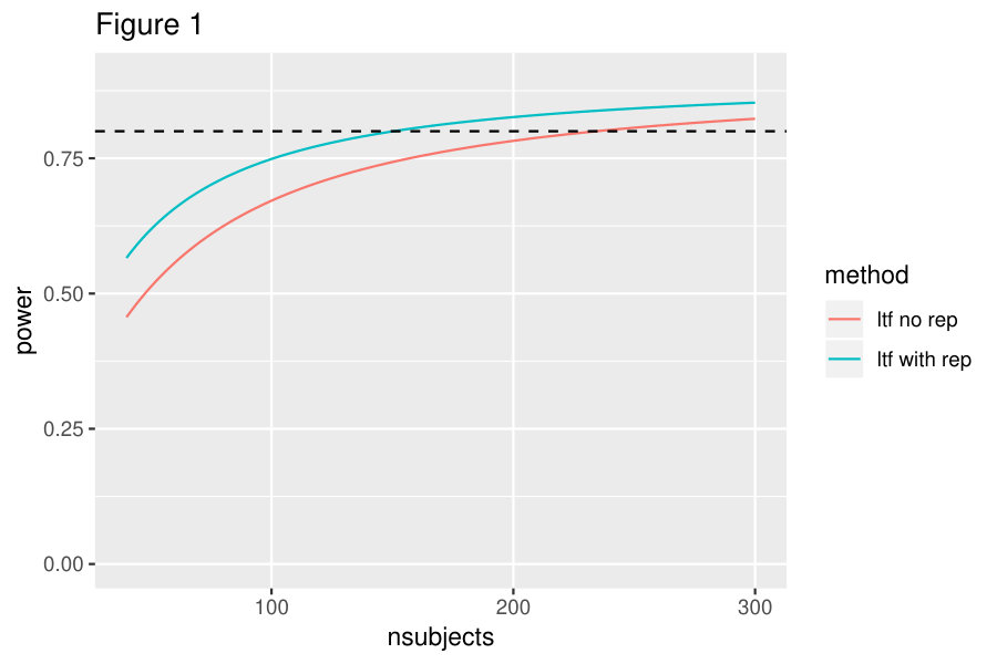 Figure 1
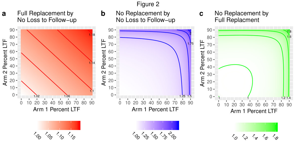 Figure 2
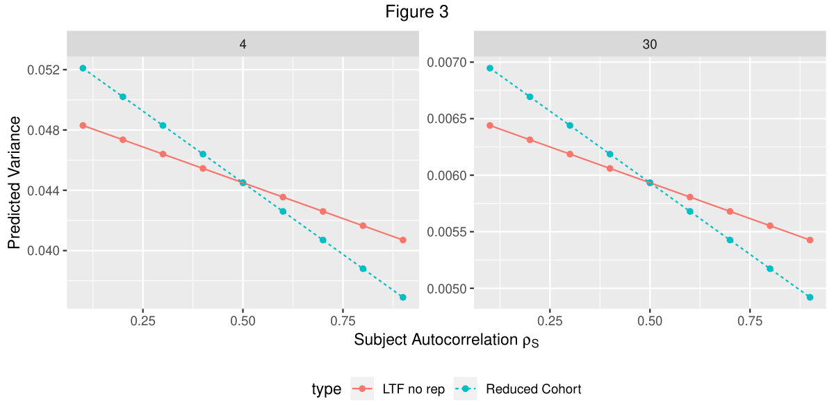 Figure 3
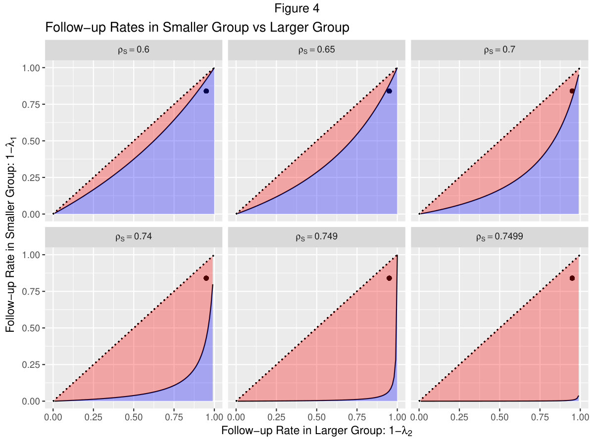 Figure 4
Peer Reviews
No public reviews on file for this paper yet. If you reviewed it on a platform where reviews are public (OpenReview, ICLR, NeurIPS, ICML), you can paste yours below so the community can read it here.
Videos
No videos yet. Explain this paper in a talk, walkthrough, or lecture? Add one.
Taxonomy
TopicsStatistical Methods in Clinical Trials · Optimal Experimental Design Methods · Economic and Environmental Valuation
Correct power for cluster-randomized difference-in-difference trials
with loss to follow-up
Jonathan Moyer and Ken Kleinman
Abstract
Cluster randomized trials with measurements at baseline can improve power over post-test only designs by using difference in difference designs. However, subjects may be lost to follow-up between the baseline and follow-up periods. While equations for sample size and variance have been developed assuming no loss to follow-up (“cohort”) and completely different subjects at baseline and follow-up (“cross-sectional”) difference in difference designs, equations have yet to be developed when some subjects are observed in both periods (“mixture” designs). We present a general equation for calculating the variance in difference in difference designs and derive special cases assuming loss to follow-up with replacement of lost subjects and assuming loss to follow-up with no replacement but retaining the baseline measurements of all subjects. Relative efficiency plots, plots of variance against subject autocorrelation, and plots of variance by follow-up rate and subject autocorrelation are used to compare cohort, cross-sectional, and mixture approaches. Results indicate that when loss to follow-up to uncommon, mixture designs are almost as efficient as cohort designs with a given initial sample size. When loss to follow-up is common, mixture designs with full replacement maintain efficiency relative to cohort designs. Finally, our results provide guidance on whether to replace lost subjects during trial design and analysis.
1. Introduction
Cluster randomized trials (CRTs) are trials in which groups or clusters of individuals are randomly assigned to treatment conditions. This is in contrast to an individually randomized trial (IRT), in which individuals themselves are randomly assigned to treatment conditions. A trial may be be conducted as a CRT for reasons of administrative convenience or to avoid cross contamination (Hayes and Moulton 2017). However, the tendency of measurements within a given cluster to be correlated that must be accounted for when when designing and analyzing a CRT. Failing to account for this will typically increase the Type 1 error rate.
The “parallel arm” CRT design consists of measuring the response after implementation of the treatment. However, it is common to record measurements of the response at baseline as well as after treatment implementation. In this situation, analysis can focus on the difference in differences (DID) - that is, the difference in change between treatment and control groups. Examples include studies in improving stroke rehabilitation (Strasser et al. 2008), dating violence prevention (Miller et al. 2012), and community-based modification of harmful gender norms (Pettifor et al. 2018). Use of the DID design can result in improvements to power (Rutterford, Copas, and Eldridge 2015).
Two classes of DID design have long been recognized (Murray and Hannan 1990). The first is the cohort design, in which the same subjects are measured at baseline and at follow-up. The second is the cross sectional design, in which subjects within a cluster at follow-up are different from those at baseline. A single expression has been developed for the variance of the DID estimator that incorporates aspects of both cohort and cross-sectional designs (Feldman and McKinlay 1994).
Mixtures of the two designs are also possible. In this scenario, individuals measured at baseline and lost to follow-up may be replaced. Thus complete observations are available for some individuals, those lost to follow-up have only baseline measurements, and the replacements have only follow-up measurements. An example is the REDUCE MRSA trial, where participating hospitals were randomly assigned to one of three strategies to prevent health-care associated infections (Huang et al. 2013). In this trial, virtually all subjects lost to follow-up were replaced with new subjects, but some subjects were present at baseline and follow-up. Previous work (Teerenstra et al. 2012), (Feldman and McKinlay 1994) mentions that the formulation for the DID estimator variance and design effect can be applied to mixtures of cohort and cross-sectional designs but does not provide further details.
Mixtures of the two designs could be considered from the perspective of missing data, which is a common occurence in CRTs (Fiero et al. 2016). That is, individuals present only at baseline have missing values at follow-up, while individuals present only at follow-up have missing values at baseline. The cross-sectional design could be considered an extreme case in which all individuals at baseline and follow-up are respectively missing their follow-up and baseline values. Another extreme case of a “mixture” design is when individuals are lost to follow-up and not replaced. In an IRT, a DID analysis must necessarily omit those lost to follow-up. However, in a CRT, those lost to follow-up still contribute to the cluster means at baseline.
The goal of this article is to develop an approach to calculating the DID estimator variance and design effect for the mixture design, including replacement of those lost to follow-up or no replacement at all. In section 2 we review the model used for the DID design. In section 3 we present variations to the variance of the DID estimator assuming replacement of drop-outs and consider power and sample size calcualtions. In section 4, we compare the variance of DID estimators using relative efficiency plots, plots of predicted variance against subject autocorrelation , and plots indicating which DID design predicts the smallest variance given pairs of follow-up rates. Finally, in section 5 we offer further discussion and concluding thoughts.
2. DID Model Review
Let be a continuous outcome for individual in cluster and treatment group at time , where is the total number of clusters per arm and is the number of individuals in cluster at time . Let and be indicators for arm ( for control, for treatment) and time ( for baseline, for follow-up). Then the model for is
[TABLE]
Fixed effects include the first four terms of equation 1, where represents the mean of the control group at baseline, is the mean baseline difference between treatment and control groups, represents the mean difference between follow-up and baseline values for the control group, and is mean differential change between treatment and control. The parameter corresponds to the DID.
Random effects are represented by the last four terms of equation 1. They are assumed to be mutually independent and normally distributed as follows:
[TABLE]
The terms and represent time-invariant and time-varying effects due to cluster, respectively. Each cluster will have one value for and two values for corresponding to baseline and follow-up. The terms and represent time-invariant and time-varying effects due to subject, respectively. As with clusters, each subject will have one value for and two values for corresponding to baseline and follow-up. Indeed, in the common case where each subject is measured once per time point, the term serves as residual error. The notation is used here to be consistent with prior work by others.
The intracluster correlation coefficient (ICC), , is a measure of the correlation between measurements within a cluster. Often used in power analysis for CRTs, in the DID setting is defined as follows:
[TABLE]
Total cluster and subject variances are partitioned into time-invariant and time-varying components through cluster and subject autocorelation coefficients and , respectively. The parameter indicates the correlation between baseline and follow-up means for a cluster, while indicates the correlation between baseline and follow-up values for an individual, conditional on cluster random effects. In terms of the random effect variances, the autocorrelation parameters are defined as:
[TABLE]
The type of DID design - cross-sectional, cohort, or mixture - is reflected in the parameter. If , then there is no correlation between baseline and follow-up subject measurements and the design is effectively cross-sectional. Values of only have meaning as a cohort design. Assuming some fraction of subjects are measured twice with autocorrelation and the rest measured only once, the subject autocorrelation for a mixture design, defined as , will also be greater than 0 but less than . (Teerenstra et al. 2012) One aim of section 3 below is to characterize to what degree is less than .
Let be the average of the realized observations of group at time . Assuming equal number of clusters per arm and an equal number of subjects across clusters (i.e, ), the estimator of the interaction term in equation 1
- denoted as - can be represented in terms of as follows:
[TABLE]
The variance of this estimator is
[TABLE]
As discussed above, for the cross-sectional design . In this case, equation 2. DID Model Review becomes
[TABLE]
3. LTF Variations on DID
We present variations on the DID design incorporating loss to follow-up (LTF) and potentially replacement. In all cases, it is assumed that data are missing completely at random (MCAR) as defined by Rubin (Rubin 1976).
3.1 General case
Let and be the numbers lost to and gained at follow-up per cluster in arm . It is possible for to be greater than . Assume the initial number of subjects in each cluster is . With respect to , the loss to follow-up and gain at follow-up rates per cluster in arm and , respectively, are given by and . Furthermore, let . Then the subject autocorrelation modified for losses to and gains at follow-up is given by (see the appendix)
[TABLE]
This allows the variance of the DID estimator modified by gains and losses to follow-up to be represented as follows:
[TABLE]
Setting and to various quantities results in variations on the variance of the DID estimator, as discussed below.
3.2 LTF with replacement and without replacement
variations
The mixture design discussed in section 2 consists of complete loss to follow-up with full-replacement. In this case, in equation 7 and . Then , where is the mean loss to follow-up rate across both arms. The variance of the DID estimator with complete loss to follow-up with full replacement, , is therefore
[TABLE]
Setting in equation 7 and assuming results in a loss to follow-up with no replacement scenario. In this case, is given by \rho_{S}^{*}=\rho_{S}-\frac{1}{4}\Big{[}\frac{\lambda_{1}}{1-\lambda_{1}}+\frac{\lambda_{2}}{1-\lambda_{2}}\Big{]}. The variance of the DID estimator with complete loss to follow-up with full replacement, , is given by
[TABLE]
3.3 Power Calculation
The power to detect DID effect with clusters per arm is given by
[TABLE]
where is the cumulative -distribution with degrees of freedom.
Using one of the subject autocorrelations described previously, one can solve for the minimum number of clusters per arm needed to attain a given power at a given level of significance .
[TABLE]
where non-centrality parameter . In practice, power calculation software, such as that provided by the clusterPower package in R, can also compute power and other quantities of interest (Kleinman, Moyer, and Reich 2017).
3.4 Example Sample Size
Determination
To illustrate the use of the preceding equations, we proceed as if we were planning an intervention to determine the effects of the dating violence preventon program described by Miller et al (2012). One goal of this study was to improve high school aged male athletes’ inclination to intervene when witnessing abusive behavior, as measured on an 8-item scale. The study was a cohort design with 16 high schools as the clustering units. At baseline, approximately 125 students per school participated. The analysis was performed on complete case data, but the authors report follow-up rates of 84% and 95% in the treatment and control groups, respectively. The adjusted mean difference in intention to intervene change was observed to be 0.12, meaning intervention youth increased intent to intervene by 0.12 points on average relative to control youth (). Correspondence with the authors indicated that the values of , , , and were 0.0218, 0.0047, 0.3342, and 0.2567, respectively. This produces values of 0.0429, 0.8226, and 0.5656 for , , and , respectively.
In our intervention, suppose we have 30 schools participating (15 per arm) and want to know the minimum number of subjects per school needed to attain 80% power at a 5% level of significance. Using the utilities in the R package clusterPower, the power for each design can be computed over a number of subjects.
Figure 1 shows the association between the number of subjects per cluster at baseline and power. The blue line denotes the loss to follow-up with replacement design (where and ) and the red line uses the loss to follow-up with no replacement design (where and \rho_{S}^{*}=\rho_{S}-\frac{1}{4}\Big{[}\frac{\lambda_{1}}{1-\lambda_{1}}+\frac{\lambda_{2}}{1-\lambda_{2}}\Big{]}). For the given parameters, the no LTF and complete case designs give power estimates very similar to the loss to follow-up with replacement design and so are not plotted here. Figure 1 indicates that for 80% power a minimum of 151 subjects per cluster is needed for the loss to follow-up with replacement design, while a minimum of 235 subjects per cluster is needed for the loss to follow-up with no replacement design.
4. Comparisons of DID
Estimators
In this section we compare versions of the DID estimators. Section 4.1 presents relative efficiency plots. Section 4.2 presents figures comparing variance as a function of subject autocorrelation , as well as indicating which DID design (reduced cohort or LTF with no replacement) yields a smaller variance for given follow-up rates.
4.1 Comparisons of DID
Estimators
Figure 2 presents relative efficiency plots for three comparisons. LTF rates for group 1 and group 2 are plotted on the - and -axes, while relative efficiency is plotted on the -axis as color. The variances and correlation coefficients used in White represents a relative efficiency of 1, while more intense color represents larger relative efficiencies. For all plots, the number of clusters per arm was 30, the number of subjects per cluster was 100 while , , , and were 0.015, 0.035, 0.76, and 0.19, respectively. The variance values correspond to an ICC of 0.05, a cluster autocorrelation of 0.3, and a subject autocorrelation of 0.8.
Figure 2a compares the LTF with full replacement variance (where and using in equation 2. DID Model Review) to that of the no LTF cohort design (). Figure 2b compares the LTF with no replacement variance (with and using \rho_{S}^{*}=\rho_{S}-\frac{1}{4}\Big{[}\frac{\lambda_{1}}{1-\lambda_{1}}+\frac{\lambda_{2}}{1-\lambda_{2}}\Big{]} in equation 2. DID Model Review) to that of the no LTF cohort design. Figure 2c compares the no replacement variance () to the full replacement variance (). In figures 2a and 2b, as percent lost to follow-up in both arms increases, the variances of the complete replacement and no replacement estimators are inflated relative to the no LTF cohort design. In both figures 2a and 2b, when percent LTF in both groups is low the variance inflation is relatively mild. For example, if 10% of units are lost to follow-up in both treatment groups, figure 2a indicates that the variance of the LTF with full replacement estimator is only about 1.02 times greater than that of no LTF cohort design. Similarly, with 10% lost to follow-up in each arm figure 2b indicates the variance of the LTF with no replacement estimator is close to 1. Indeed, at even fairly high loss to follow-up percentages the inflation factor for the full replacement variance is low. For example, if the percent lost to follow-up is 80%, figure 2a indicates that the LTF with replacement estimator variance is only about 1.035 times that of the no LTF cohort design. However, figure 2b indicates that, with an 80% loss to follow-up in both treatment groups, the variance of the LTF with no replacement estimator is approximately 1.2 times that of the no LTF cohort. Given that the inflation factors depicted in figure 2a remain fairly close to 1, it’s not surprising that figure 2c bears a stronger resemblance to figure 2b.
In figure 2c, the lower left region of the plot indicates that the full replacement variance is slightly less than the the no replacement variance. An explanation for this observation is that the larger sample size of the full replacement scenario does not overcome the added uncertainty brought about by gaining new individuals at follow-up.
4.2 Comparison of Reduced Cohort and LTF with no replacement
Designs
A common strategy for power calculation is to assume a cohort design using the expected cluster size at follow-up, assuming no LTF. In effect, individuals who were present at baseline but not at follow-up are discarded in the power calculation. If the data are MCAR this won’t introduce bias, but the smaller sample size will reduce power. The variance for this calculation is given by equation 2. DID Model Review, using the expected follow-up cluster size for . This will be referred to as the reduced cohort DID design.
An alternative would be to use the LTF with no replacement formula give in equation 3.2 LTF with replacement and without replacement variations, which uses the baseline observations of individuals lost to follow-up. Given that the total sample size in this equation is greater than the reduced cohort case, it might be expected to produce a lower variance, and therefore greater power, for a given effect size. This will be referred to as the LTF with no replacement DID design.
Here we compare the DID estimator variance of the reduced cohort design with the variance of the LTF with no replacement design. Figure 3 displays variances plotted against subject autocorrelation for the LTF no replacment design (100 subjects per cluster at baseline, 50 per cluster lost to follow-up) and the reduced cohort (50 subjects per cluster at baseline and follow-up), with treatment and control groups having 4 and 30 clusters each. Cluster autocorrelation, cluster variance, and subject variance were set at 0.3, 0.05, and 0.95, respectively. Despite having a smaller overall sample size, at values of greater than 0.5 the DID estimator from the smaller reduced cohort design has less variance than the LTF with no replacement design.
Another scenario of interest is when loss to follow-up is different for treatment and control arms. Let be the DID estimator in the reduced cohort scenario. Let be the DID estimator in the LTF with no replacement scenario. Let be the sample size per cluster for both treatment and control at baseline, so all clusters have the same size at baseline. Let and be the sample sizes per cluster the control and treatment groups at follow-up, respectively. Suppose the cluster sizes in each arm are different - without loss of generality, . Then the following inequality
[TABLE]
is true when
[TABLE]
That is, when the follow-up rate in the small group is greater than the value given on the right hand side of inequality 13, the variance of the reduced cohort scenario will be less than that given by the LTF with no replacement scenario.
Figure 4 plots follow-up rates in the smaller group versus follow-up rates in the larger group for several values of . The dashed diagonal line is the identity line and correpsonds to a of 0.50. Values of below 0.50 and above 0.75 are not shown as they produce follow-up rates in the smaller group that either less than 0 or are greater than those in the larger group. The dot at (0.95, 0.84) represents the follow-up rates for the two arms in the trial described by Miller et al (2012) and is discussed further below.
Combinations of follow-up rates in this red region (above the solid line) indicate that variance for the reduced cohort DID estimator is less than the variance in the LTF with no replacement DID estimator. Therefore, sample size calculations for combinations in this region should use the variance given in equation 2. DID Model Review, using the minimum of treatment or control follow-up cluster size for . In addition, analyses should omit those lost to follow-up.
The blue shaded regions correspond to combinations of follow-up rates and that don’t satisfy inequality 13. In these regions, the variance of the reduced cohort DID estimator will be greater than that of the LTF with no replacement DID estimator should be used. These plots serve as a useful tool for selecting a method to calculating variance and determining which approach to use in order to minimize participant risk while still attaining the desired power.
For example, consider the study by Miller et al (2012) in which the follow-up rates in the two arms were 95% and 84% (represented by the dot in figure 4) and is slightly less than 0.60. These settings result in placement in the blue region of the top left plot in figure 4. This suggests the LTF with no replacement DID estimator has the smaller variance than that of the reduced cohort DID estimator. However, suppose was 0.70 but the follow-up rates were the same. In this situation, placement would now be in the red region in the top right plot in figure 4. This indicates that reduced cohort DID variance will be smaller than the LTF with no replacement DID variance.
Other observations from figure 4 include the following. For values of , the blue region occupies everything under the line of identity and the LTF with no replacement approach will yield the smallest variance for any combination of follow-up rates. If and the follow-up rates per cluster between the two groups are the same, then the line of identity will always be in the red region and the reduced cohort calculation should be used. For values of , the region under the line of identity will be completely red and the reduced cohort variance computation should be used.
5. Conclusion
Relative to the no loss to follow-up (LTF) cohort design, the LTF with replacement scenario results in mild variance inflation for even relatively high LTF rates, as shown in Figure 2. In situations where it is costly or difficult to maintain a cohort but replacements from within clusters can be found, the LTF with replacement mixture design appears to be an acceptable approach. During study design, when finding a needed sample size for the LTF with replacement scenario, one can estimate the variance with equation 2. DID Model Review by multiplying the expected subject autocorrelation by the expected mean follow-up rate as shown in equation 3.2 LTF with replacement and without replacement variations.
The LTF with no replacement scenario also results in only mild variance inflation relative to no LTF cohort design if LTF rates are low in both control and treatment arms. However, high LTF rates in at least one of the arms in the LTF with no replacement scenario results in substantial variance inflation. Interestingly, the LTF with no replacement design is more efficient than the LTF with full replacement design when the loss to follow-up rates are very low. The larger sample size in the full replacement scenario does not overcome the added uncertainty brought about by obtaining new individuals at follow-up.
When comparing LTF with no replacement and reduced cohort designs, low values of indicate that the former has a smaller predicted variance while large values of indicate the opposite is true, as shown in Figure 3. Typically, there is no a priori expectation of different loss to follow-up in each treatment group. Thus, when is expected to be below 0.5, the LTF with no replacement DID approach is recommended. One can then use equation 3.2 LTF with replacement and without replacement variations to compute the variance of the DID estimator. Otherwise, if is expected to be greater than 0.5, the reduced cohort design is preferred.
Our results also show that, in general, the LTF with no replacement scenario outperforms the reduced cohort case when the subject autocorrelation is low and loss to follow-up rates are high, as shown in Figure 4. However, when is large and LTF rates are low, the reduced cohort design yields a smaller variance. In these situations, the strong subject autocorrelation provides more information through the DID estimator than that provided from the means at baseline and follow-up. In practice, with estimates of and the follow-up rates in each arm, Figure 4 can be used to determine which design - LTF with no replacement or reduced cohort - is preferred over the other. Follow-up rates and values resulting in placement in the red region indicate that the reduced cohort design is preferred, while placement in the blue region indicates that the LTF with no replacement design is preferred.
A limitation of the methods discussed above is that the variance parameters , , , and are rarely all reported in study results. Knowledge of these four parameters is needed for finding the ICC, , and parameters. In addition, not all cohort designs may have replacement subjects available, limitind consideration to the no LTF and reduced cohort settings.
In summary, our results indicate that if individuals are available to replace those lost to follow-up, the LTF with replacement design performs similarly to the no LTF design. An exception is when the loss to follow-up rates in each arm are relatively low. In this case the LTF with no replacement design has a smaller variance. If it is not possible to replace those lost to follow-up, then the choice of using the LTF with no replacement and reduced cohort designs depends largely on the magnitude of subject autocorrelation . If is expected to be below 0.50, the LTF with no replacement design should be used. If is larger than 0.50 and the follow-up rates in the arms are expected to be very different, then the LTF with no replacement design is likely to be preferred. However, if is large and the follow-up rates in each arm are expected to be the same or similar, the reduced cohort design is preferred. Finally, if is expected to be very large (greater than 0.75), then the reduced cohort design should be used regardless of the follow-up rates in each arm.
Appendix
A.1 DID Estimator
Let be the number of clusters per arm. Let be the number of subjects in cluster at time . Define the mean of arm () at time () as:
[TABLE]
and , , , and . Then the DID estimator is given by
[TABLE]
The variance of the DID estimator is:
[TABLE]
because for , Cov() = 0.
The cluster variance of the mean response for arm at time , , is given by:
[TABLE]
because for , Cov() = 0.
For arm , the covariance between mean response at baseline and follow-up is given by
[TABLE]
The expressions given in equations A.1 DID Estimator and A.1 DID Estimator do not make assumptions about cluster sizes. In subsequent sections we will make simplifying assumptions about the cluster sizes.
A.2 DID Estimator with modifications for loss to follow-up
and replacement
In this section we derive the variance for the loss to follow-up (LTF) with partial repalcement scenario with variable LTF for each cluster. In this setting the cluster at baseline contains individuals, loses individuals at follow-up, and partially replaces individuals at follow-up. A matrix of the cluster is presented below (the subscripts are omitted for clarity).
{\sigma^{2}}$${\sigma^{2}}$${\sigma_{C}^{2}}$${\sigma_{C}^{2}}$${\sigma^{2}}$${\sigma^{2}}$${\sigma_{C}^{2}}$${\sigma^{2}}$${\sigma^{2}}$${\sigma^{2}}$${\sigma^{2}}$${\sigma_{C}^{2}}$${\sigma^{2}}$$\left[\vbox{\hrule height=98.36902pt,depth=98.36902pt,width=0.0pt}\right.$$\left.\vbox{\hrule height=98.36902pt,depth=98.36902pt,width=0.0pt}\right]
\left\{\vbox{\hrule height=27.24582pt,depth=27.24582pt,width=0.0pt}\right.$$L$$\left\{\vbox{\hrule height=31.38031pt,depth=31.38031pt,width=0.0pt}\right.$$K-L$$\left\{\vbox{\hrule height=31.38031pt,depth=31.38031pt,width=0.0pt}\right.$$K-L$$\left\{\vbox{\hrule height=24.7143pt,depth=24.7143pt,width=0.0pt}\right.$$G$$\left\{\vbox{\hrule height=25.95917pt,depth=25.95917pt,width=0.0pt}\right.$$L$$\left\{\vbox{\hrule height=27.86469pt,depth=27.86469pt,width=0.0pt}\right.$$K-L$$\left\{\vbox{\hrule height=23.85303pt,depth=23.85303pt,width=0.0pt}\right.$$K-L$$\left\{\vbox{\hrule height=20.99867pt,depth=20.99867pt,width=0.0pt}\right.$$G
where . The upper left and lower right quadrants of this matrix (enclosed in light gray boxes) represent cluster covariances at baseline and follow-up, respectively. In the area enclosed by the light gray boxes, all off-diagonal elements are . The off-diagonal blocks represent covariances from baseline to follow-up. The covariance parameter indicated within a submatrix demarcated by dashed lines implies that all elements in that submatrix are that covariance value.
The table below shows the covariances for cluster at time .
[TABLE]
At baseline, there are blocks, so for cluster the sum of the covariances is:
[TABLE]
Thus equation A.1 DID Estimator becomes:
[TABLE]
For clusters at follow-up, the result is similar, save that the cluster size at follow-up is . So
[TABLE]
Because the denominators are not all the same, equation A.2 DID Estimator with modifications for loss to follow-up and replacement cannot be simplified further. We need to make assumptions about the ’s to proceed. In the preceding section we assumed and for any and . This means that the losses to follow-up for each cluster are the same and the numbers replaced at follow-up for each cluster are the same, but the number of replacments does not necessary equal the number lost. Here we assume that the loss to follow-up and replacement at follow-up varies by treatment arm. Thus for arm we have
[TABLE]
where and are the number lost to follow-up and replaced at follow-up, respectively, in arm .
The covariances for observations in cluster across time are given in the following tables:
[TABLE]
In the block of the preceding table, the “Sum in Block” is instead of to avoid double counting cases in the intersection with the block.
For , the sum of the covariances is . For , the sum of the covariances is . Thus the sum of the covariances for cluster across time is:
[TABLE]
Thus the covariance becomes:
[TABLE]
Using the results from equations 21 and A.2 DID Estimator with modifications for loss to follow-up and replacement, equation A.1 DID Estimator becomes:
[TABLE]
Loss to follow-up with complete
replacement
Here it is convenient to pause and derive the variance of the loss to follow-up with full replacement estimator. In this case, so equation A.2 DID Estimator with modifications for loss to follow-up and replacement becomes
[TABLE]
where .
Loss to follow-up with no or partial
replacement
In the case of loss to follow-up with no or partial replacement, we continue from equation A.2 DID Estimator with modifications for loss to follow-up and replacement as follows:
[TABLE]
Letting , we get
[TABLE]
where is the loss to follow-up per cluster in group and is the gain at follow-up (relative to the initial cluster size, ) per cluster in group .
If \rho_{S}*=\rho_{S}-\frac{1}{4}\Big{[}\frac{1}{1-\lambda_{1}+\gamma_{1}}+\frac{1}{1-\lambda_{2}+\gamma_{2}}-2\frac{\eta\sigma_{S}^{2}+\sigma_{ST}^{2}}{\sigma_{S}^{2}+\sigma_{ST}^{2}}\Big{]}, then we can write
[TABLE]
References
Feldman, Henry A., and Sonja M. McKinlay. 1994. “Cohort Versus Cross-Sectional Design in Large Field Trials: Precision, Sample Size, and a Unifying Model.” Statistics in Medicine 13 (1):61–78. https://doi.org/10.1002/sim.4780130108.
Fiero, Mallorie H., Shuang Huang, Eyal Oren, and Melanie L. Bell. 2016. “Statistical Analysis and Handling of Missing Data in Cluster Randomized Trials: A Systematic Review.” Trials 17 (72). https://doi.org/10.1186/s13063-016-1201-z.
Hayes, Richard J., and Lawrence H. Moulton. 2017. Cluster Randomized Trials. 2nd ed. CRC Press.
Huang, Susan S., Edward Septimus, Ken Kleinman, Julia Moody, Jason Hickok, Taliser R. Avery, Julie Lankiewicz, et al. 2013. “Targeted Versus Universal Decolonization to Prevent Icu Infection.” New England Journal of Medicine 368 (24):2255–65. https://doi.org/10.1056/NEJMoa1207290.
Kleinman, Ken, Jon Moyer, and Nicholas Reich. 2017. ClusterPower: Power Calculations for Cluster-Randomized and Cluster-Randomized Crossover Trials. https://CRAN.R-project.org/package=clusterPower.
Miller, Elizabeth, Daniel J Tancredi, Heather L McCauley, Michele R Decker, Maria Catrina D Virata, Heather A Anderson, Nicholas Stetkevich, Ernest W Browne, Feroz Moideen, and Jay G Silverman. 2012. “Coaching Boys into Men: A Cluster-Randomized Controlled Trial of a Dating Violence Prevention Program.” Journal of Adolescent Health 51 (5):431–38. https://doi.org/10.1016/j.jadohealth.2012.01.018.
Murray, David M., and Peter J. Hannan. 1990. “Planning for the Appropriate Analysis in School-Based Drug-Use Prevention Studies.” Journal of Consulting and Clinical Psychology 58 (4):458–68. https://doi.org/http://dx.doi.org/10.1037/0022-006X.58.4.458.
Pettifor, Audrey, Sheri A. Lippman, Ann Gottert, Chirayath M. Suchindran, Selin Amanda, Dean Peacock, Suzanne Maman, et al. 2018. “Community Mobilization to Modify Harmful Gender Norms and Reduce Hiv Risk: Results from a Community Cluster Randomized Trial in South Africa.” Journal of the International AIDS Society 21 (7):e25134. https://doi.org/10.1002/jia2.25134.
Rubin, Donald B. 1976. “Inference and Missing Data.” Biometrika 63 (1):581–92. https://doi.org/10.1093/biomet/63.3.581.
Rutterford, Clare, Andrew Copas, and Sandra Eldridge. 2015. “Methods for Sample Size Determination in Cluster Randomized Trials.” International Journal of Epidemiology 44 (3):1051–67. https://doi.org/10.1093/ije/dyv113.
Strasser, Dale C, Judith A Falconer, Alan B Stevens, Jay M Uomoto, Jeph Herrin, Susan E Bowen, and Andrea B Burridge. 2008. “Team Training and Stroke Rehabilitation Outcomes: A Cluster Randomized Trial.” Archives of Physical Medicine and Rehabilitation 89 (1):10–15. https://doi.org/10.1016/j.apmr.2007.08.127.
Teerenstra, Steven, Sandra Eldridge, Maud Graff, Ester deHoop, and George F. Born. 2012. “A Simple Sample Size Formula for Analysis of Covariance in Cluster Randomized Trials.” Statistics in Medicine 31 (20):2169–78. https://doi.org/10.1002/sim.5352.