Dynamics of shadow system of a singular Gierer-Meinhardt system on an evolving domain
Nikos. I. Kavallaris, Raquel Barreira, Anotida Madzvamuse

TL;DR
This paper investigates the complex dynamics of a shadow system derived from a singular Gierer-Meinhardt model on an evolving domain, focusing on blow-up phenomena, pattern formation, and stability analysis, supported by numerical simulations.
Contribution
It introduces a reduced non-local equation for the shadow system on an evolving domain and analyzes its blow-up behavior and pattern stability, extending understanding of reaction-diffusion systems.
Findings
Identification of diffusion-driven blow-up in the non-local equation.
Observation of Turing instability near stationary solutions.
Numerical confirmation of theoretical results and comparison with stationary domain cases.
Abstract
The main purpose of the current paper is to contribute towards the comprehension of the dynamics of the shadow system of a singular Gierer-Meinhardt model on an isotropically evolving domain. In the case where the inhibitor's response to the activator's growth is rather weak, then the shadow system of the Gierer-Meinhardt model is reduced to a single though non-local equation whose dynamics is thoroughly investigated throughout the manuscript. The main focus is on the derivation of blow-up results for this non-local equation, which can be interpreted as instability patterns of the shadow system. In particular, a {\it diffusion-driven instability (DDI)}, or {\it Turing instability}, in the neighbourhood of a constant stationary solution, which then is destabilised via diffusion-driven blow-up, is observed. The latter indicates the formation of some unstable patterns, whilst some…
Click any figure to enlarge with its caption.
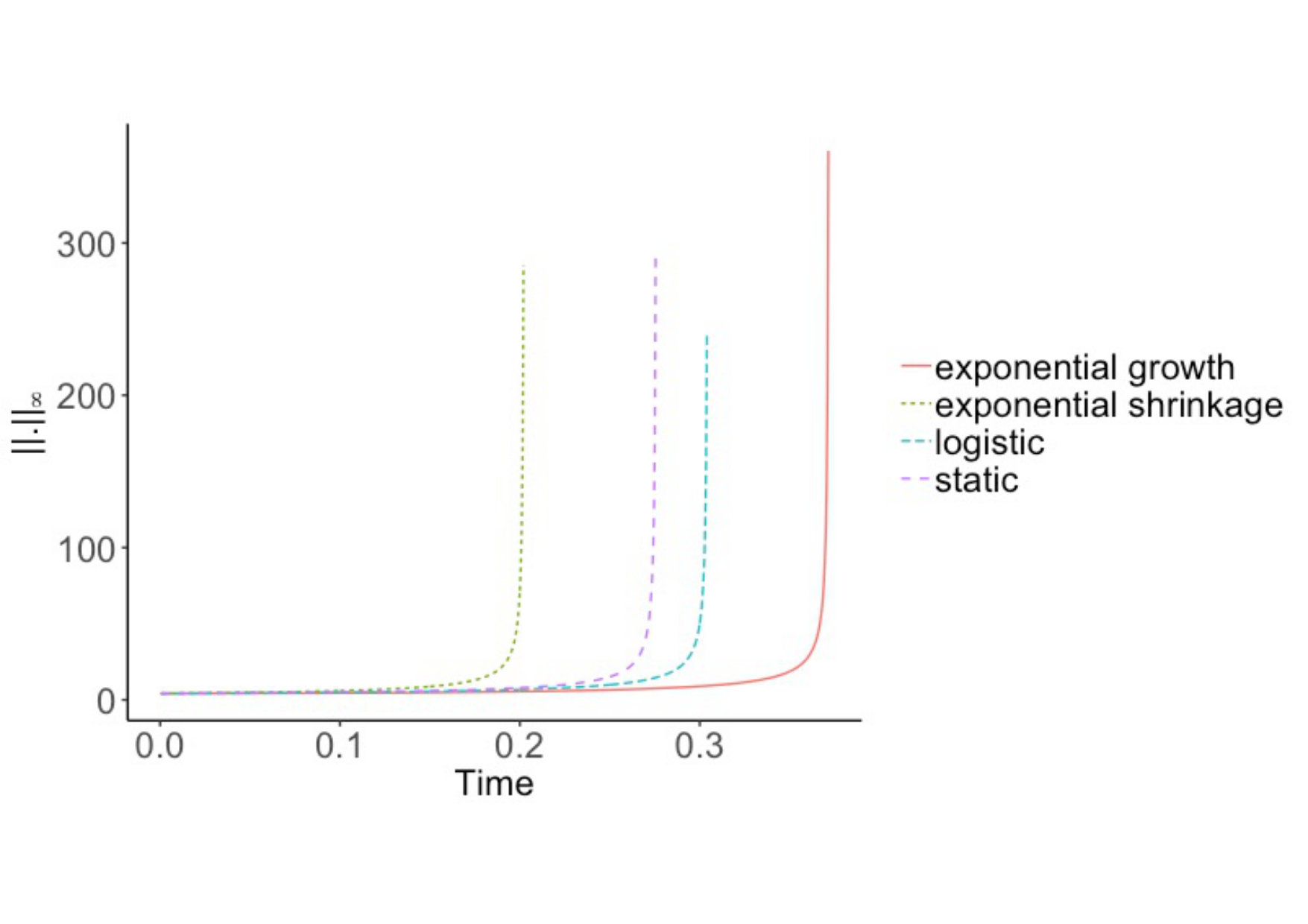 Figure 1
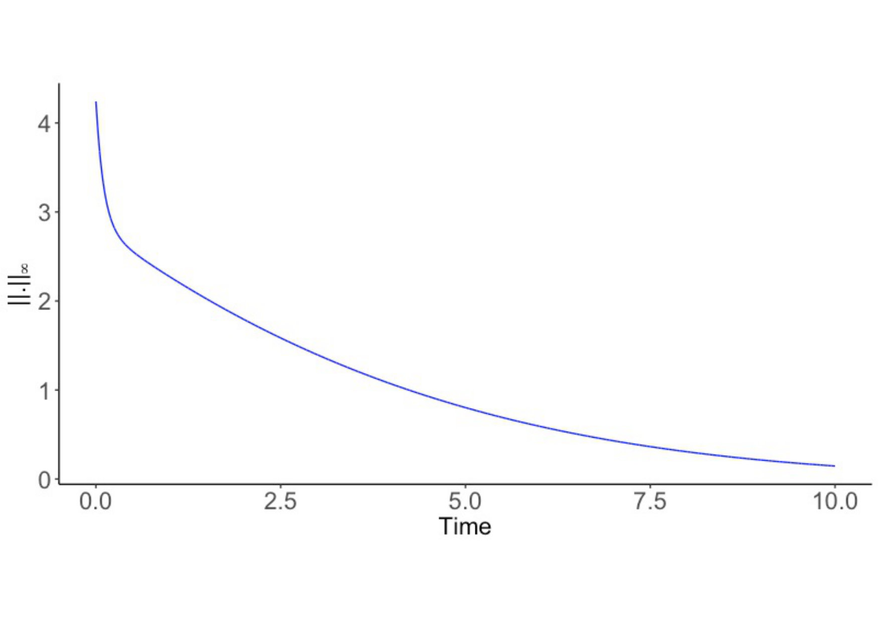 Figure 2
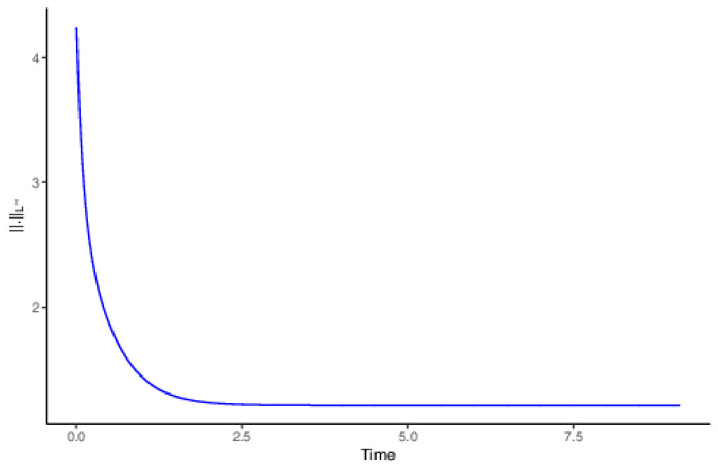 Figure 2
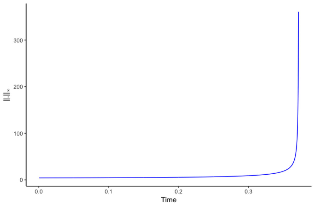 Figure 2
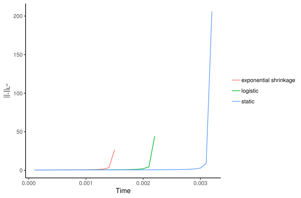 Figure 3
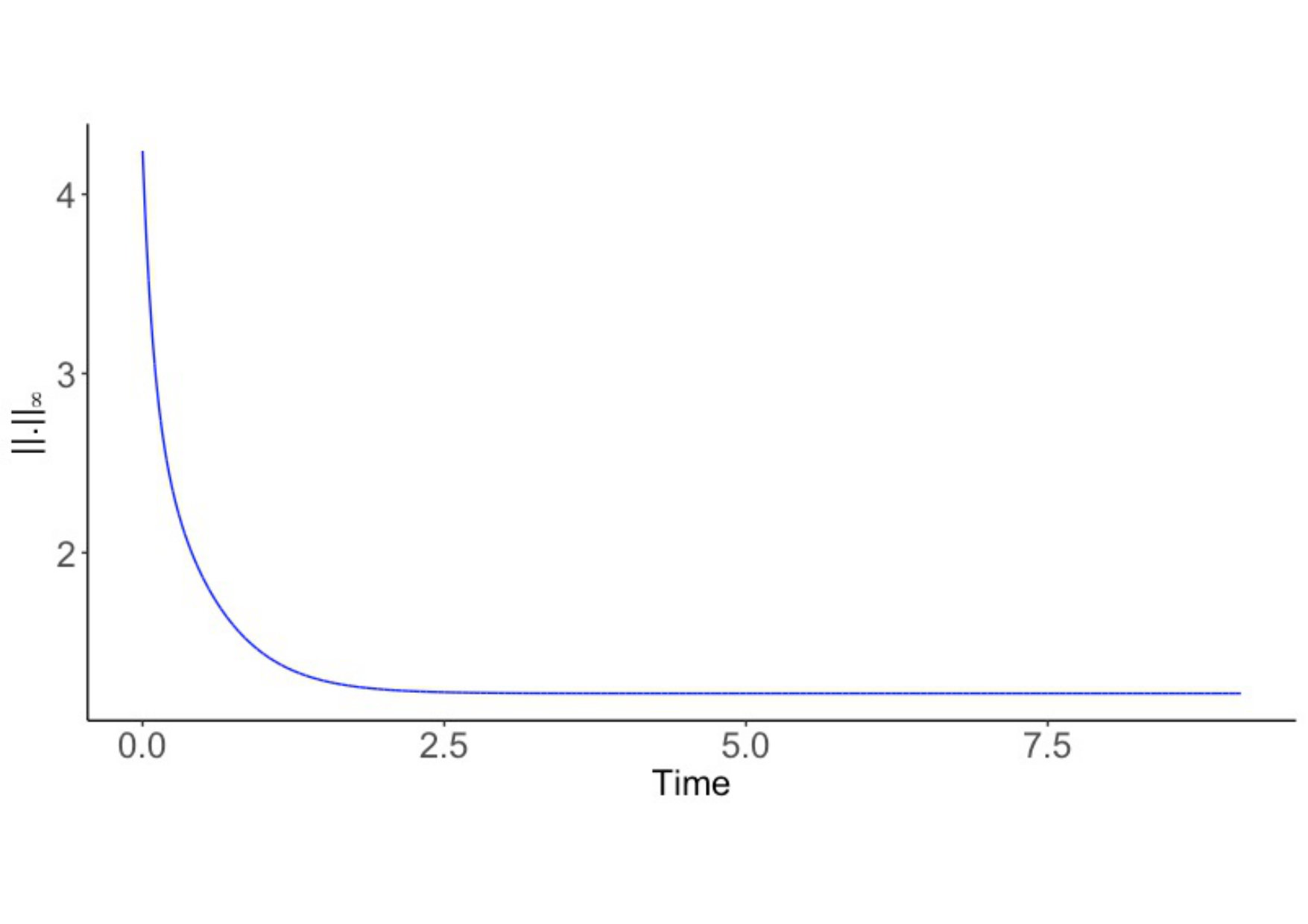 Figure 3
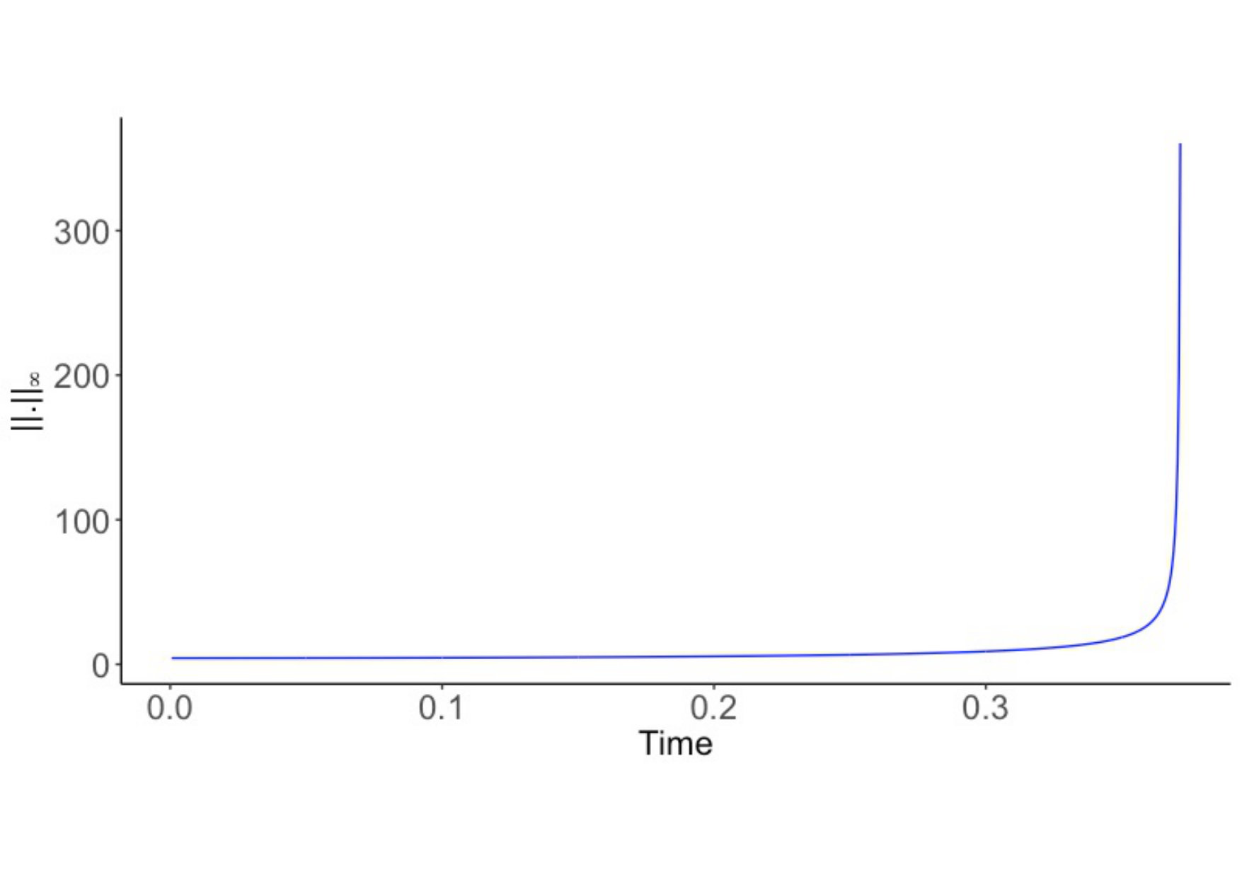 Figure 3
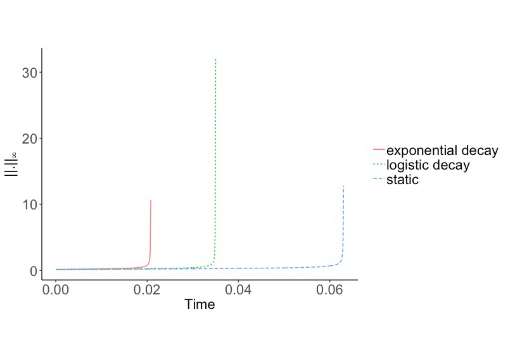 Figure 4
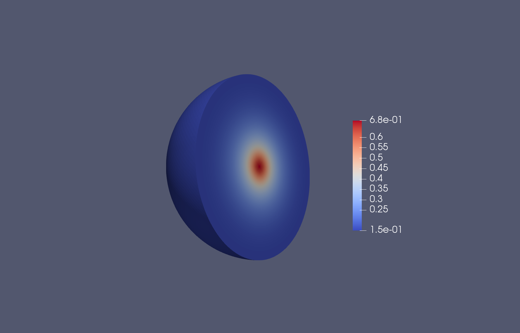 Figure 5
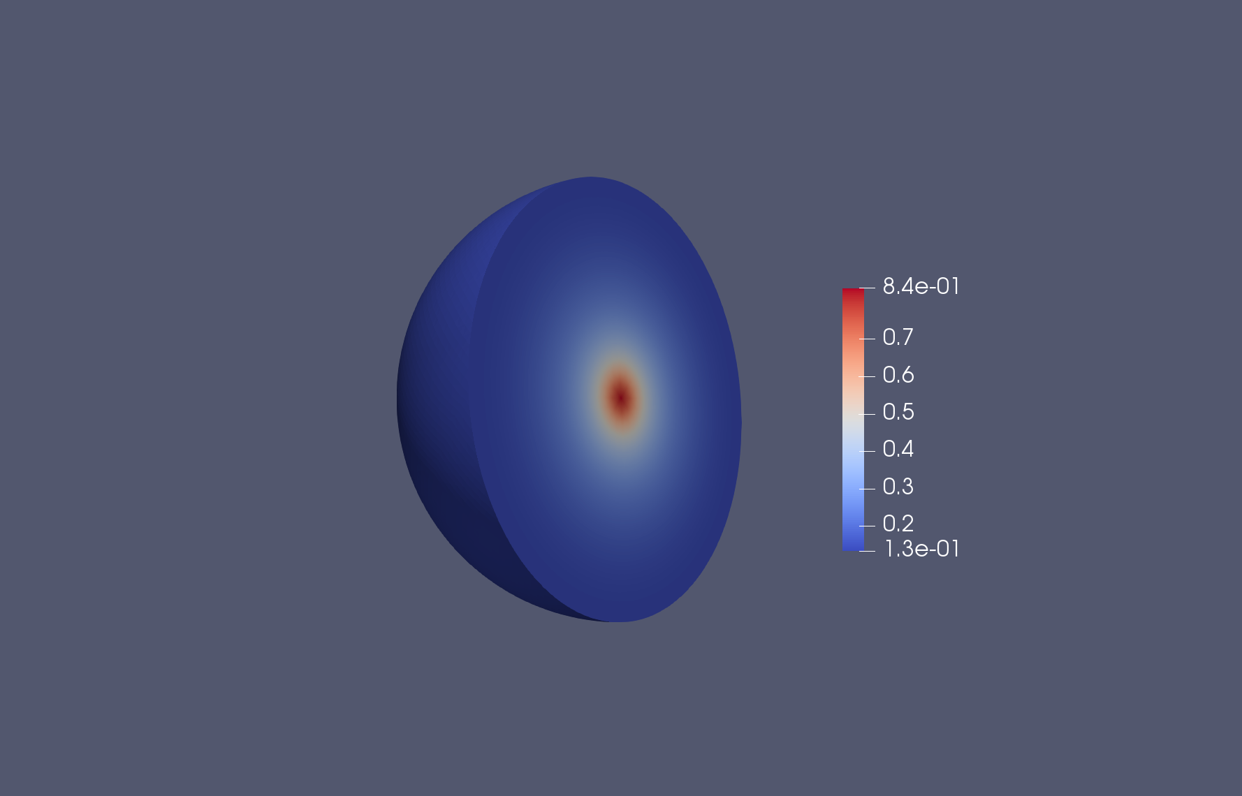 Figure 5
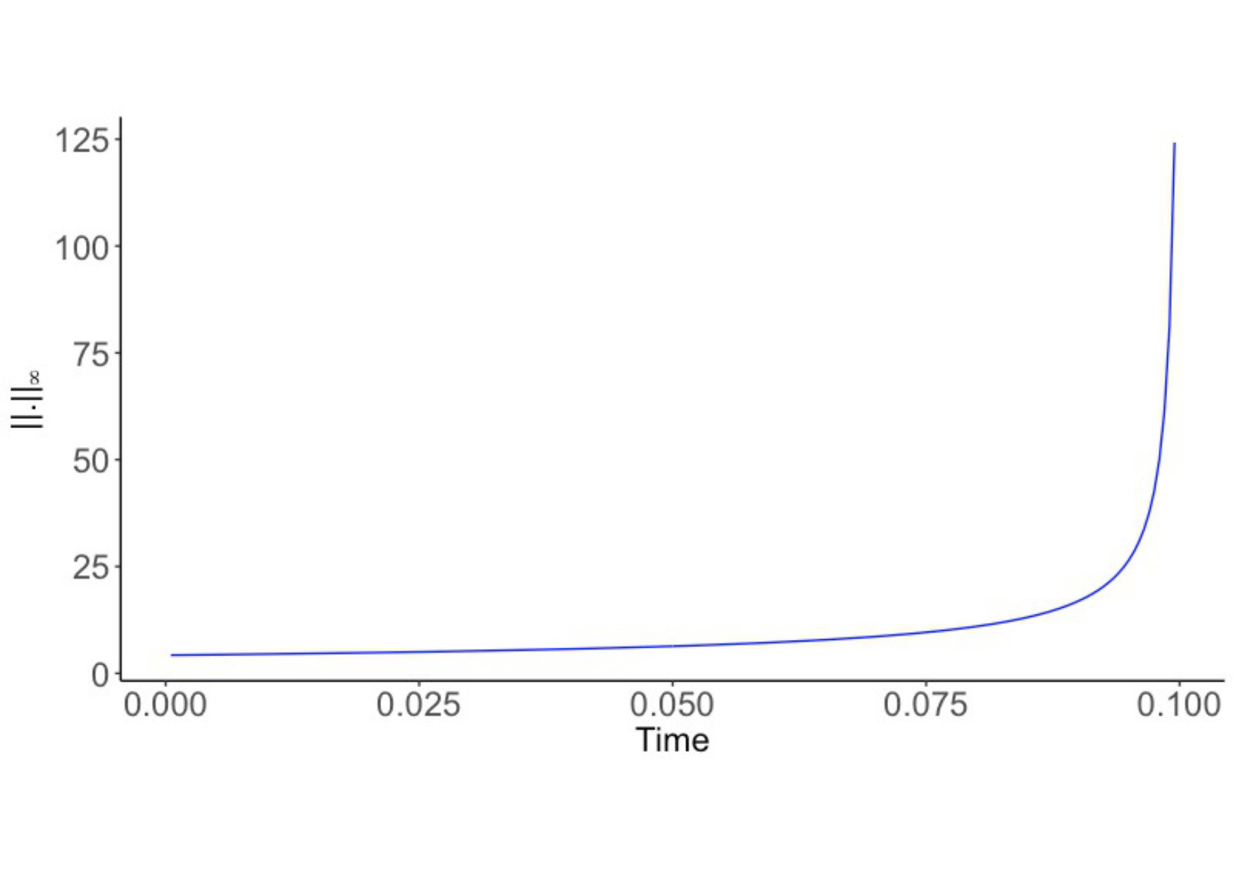 Figure 6
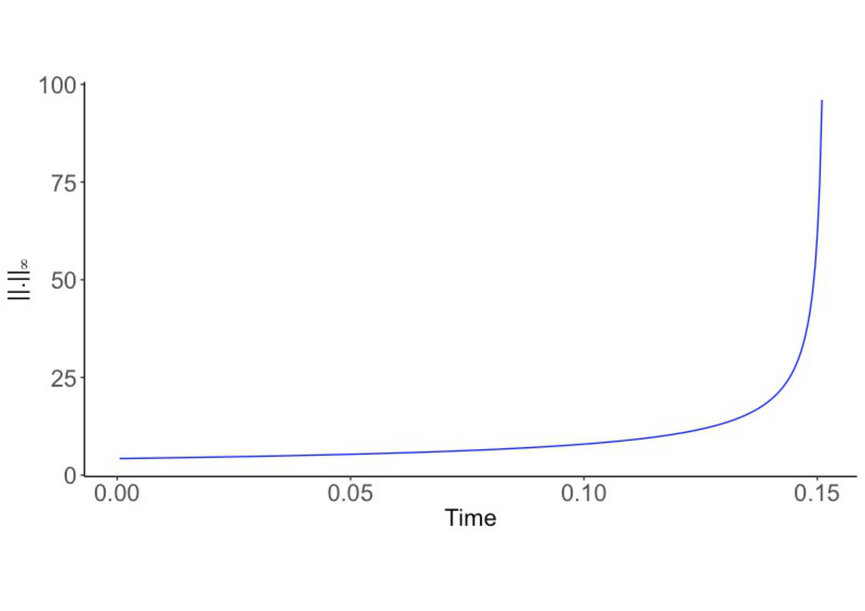 Figure 6
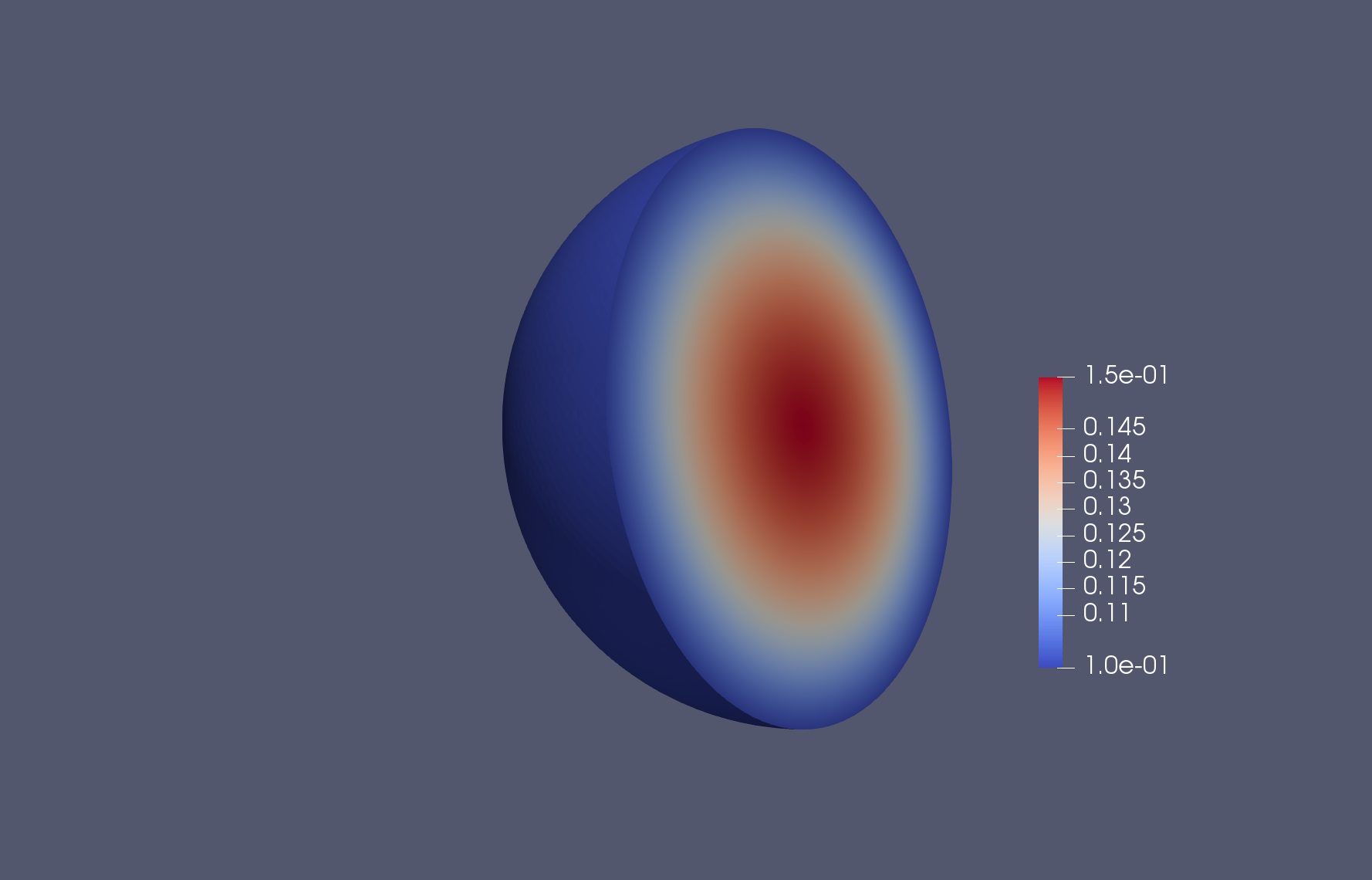 Figure 13
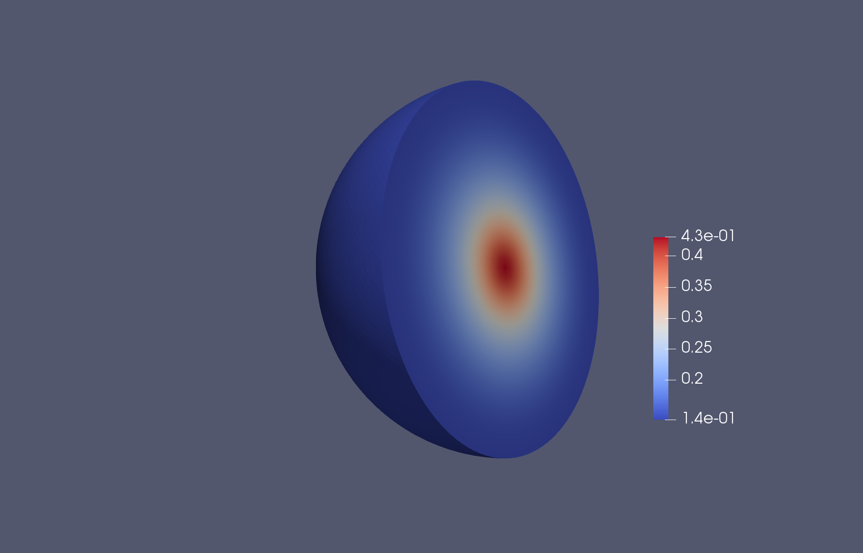 Figure 14
| 1 | 3 | 2 | 1 | 2 | 0.1 | 1.5 |
| conditions of Th. 2.3 | |||||
|---|---|---|---|---|---|
| are verified | 1 | 1 | 2 | 3 | 2 |
| are not verified | 1 | 3 | 2 | 1 | 1 |
Peer Reviews
No public reviews on file for this paper yet. If you reviewed it on a platform where reviews are public (OpenReview, ICLR, NeurIPS, ICML), you can paste yours below so the community can read it here.
Videos
No videos yet. Explain this paper in a talk, walkthrough, or lecture? Add one.
Dynamics of shadow system of a singular Gierer-Meinhardt system on an evolving domain
Nikos I. Kavallaris
Department of Mathematics, University of Chester, Thornton Science Park Pool Lane, Ince, Chester CH2 4NU, UK
,
Raquel Bareira
Barreiro School of Technology of the Polytechnic Institute of Setubal
Rua Americo da Silva Marinho-Lavradio, 2839-001 Barreiro, Portugal
and CMAFcIO - Center of Mathematics, Fundamental Applications and Operations Research, University of Lisbon, Portugal
and
Anotida Madzvamuse
School of Mathematical and Physical Sciences
Department of Mathematics
University of Sussex
Falmer, Brighton, BN1 9QH, England, UK
Abstract.
The main purpose of the current paper is to contribute towards the comprehension of the dynamics of the shadow system of a singular Gierer-Meinhardt model on an isotropically evolving domain. In the case where the inhibitor’s response to the activator’s growth is rather weak, then the shadow system of the Gierer-Meinhardt model is reduced to a single though non-local equation whose dynamics is thoroughly investigated throughout the manuscript. The main focus is on the derivation of blow-up results for this non-local equation, which can be interpreted as instability patterns of the shadow system. In particular, a diffusion-driven instability (DDI), or Turing instability, in the neighbourhood of a constant stationary solution, which then is destabilised via diffusion-driven blow-up, is observed. The latter indicates the formation of some unstable patterns, whilst some stability results of global-in-time solutions towards non-constant steady states guarantee the occurrence of some stable patterns. Most of the derived results are confirmed numerically and also compared with the ones in the case of a stationary domain.
Key words and phrases:
Pattern formation, Turing instability, activator-inhibitor system, shadow-system, invariant regions, diffusion-driven blow-up, evolving domains
Key words and phrases:
Pattern formation, Turing instability, activator-inhibitor system, shadow-system, invariant regions, diffusion-driven blow-up, evolving domains
1991 Mathematics Subject Classification:
Primary: 35B44, 35K51 ; Secondary: 35B36, 92Bxx
1991 Mathematics Subject Classification:
Primary: 35B44, 35K51 ; Secondary: 35B36, 92Bxx
1. Introduction
The purpose of the current work is to study an activator-inhibitor system, introduced by Gierer and Meinhard in 1972 [5] to describe the phenomenon of morphogenesis in hydra, on an evolving domain. Assume that stands for the concentration of the activator, at a spatial point at time which enhances its own production and that of the inhibitor. On the other hand, let represents the concentration of the inhibitor, which suppresses its own production as well as that of the activator. Hence, the interaction between and can be described by the following non-dimensionalised system [5]
[TABLE]
where is the unit normal vector on , whereas stands for the convection velocity which is induced by the material deformation due to the evolution of the domain. Moreover, are the diffusion coefficients of the activator and inhibitor respectively; represents the response of the inhibitor to the activator’s growth. Moreover, the exponents satisfying the conditions: measure the interactions between morphogens. The dynamics of system (1.1)-(1.4) can be characterised by two values: the net self-activation index and the net cross-inhibition index Index correlates the strength of self-activation of the activator with the cross-activation of the inhibitor. Thus, if is large, then the net growth of the activator is large no matter the growth of the inhibitor. The parameter measures how strongly the inhibitor suppresses the production of the activator and that of itself. If is large then the production of the activator is strongly suppressed by the inhibitor. Finally, the parameter quantifies the inhibitor’s response against the activator’s growth. Guided by biological interpretation as well as by mathematical reasons, we assume that the parameters satisfy the condition
[TABLE]
which in the literature is known as the Turing condition since it guarantees the occurrence of Turing patterns for the system (1.1)-(1.4) on a stationary domain [14].
For analytical purposes, in the current work we will only consider the case of an isotropic flow on an evolving domain, and thus we have for any :
[TABLE]
with being function with In the case of a growing domain we have whilst when the domain shrinks or for domain contraction Furthermore, the following equality holds
[TABLE]
Setting and then using the chain rule as well as (1.6) and (1.7), see also [12], we obtain:
[TABLE]
whilst similar relations hold for as well. Therefore (1.1)-(1.4) is reduced to following system on a reference stationary domain
[TABLE]
where represents the Laplacian on the reference static domain Henceforth, without any loss of generality we will omit the index from the Laplacian.
Defining a new time scale [10],
[TABLE]
and setting then system (1.8)-(1.11) can be written as
[TABLE]
where and thus and
Now if i.e. when the inhibitor diffuses much faster than the activator, then system (1.13)-(1.16) can be fairly approximated by an ODE-PDE system with a non-local reaction term. We will denote the new approximation by shadow system as coined in [9]. Below we provide a rather rough derivation of the shadow system, while for a more rigorous approach one can appeal to the arguments in [1]. Indeed, dividing (1.14) by and taking see also [15], then it follows that solves for any fixed Due to the imposed Neumann boundary condition then is a spatial homogeneous (independent of ) solution, i.e. and thus (1.14) can be written as
[TABLE]
where
[TABLE]
Averaging (1.17) over we finally infer that the pair satisfies the shadow system
[TABLE]
where \hbox to0.0pt{-\hss}\!\int_{\Omega_{0}}\tilde{u}^{r}\,d\xi=\frac{1}{|\Omega_{0}|}\int_{\Omega_{0}}\tilde{u}^{r}\,d\xi. In the limit case i.e. when the inhibitor’s response to the growth of the activator is quite small, then the shadow system is reduced to a single, though, non-local equation. Indeed, when , (1.20) entails that \eta(\sigma)=\left(\frac{\phi^{2}(\sigma)}{\Phi(\sigma)}\hbox to0.0pt{-\hss}\!\int_{\Omega_{0}}\tilde{u}^{r}\,d\xi\right)^{\frac{1}{s+1}}, and thus (1.19)-(1.22) reduce to
[TABLE]
recalling and
[TABLE]
Recovering the variable entails that the following partial differential equation holds
[TABLE]
where We note that formulation (1.23)-(1.25) is more appropriate for the demonstrated mathematical analysis, however all of our theoretical results can be directly interpreted in terms of the equivalent formulation (1.27)-(1.29). Besides, formulation (1.27)-(1.29) is more appropriate for our numerical experiments since the calculation of the functions and is not always possible.
The main aim of the current work is to investigate the long-time dynamics of the non-local problem (1.23)-(1.25) and then check whether it resembles that of the reaction-diffusion system (1.13)-(1.16). Biologically speaking we will investigate whether, under the fact that the inhibitor’s response to the growth of the activator is quite small and when it also diffuses much faster than the activator, is it necessary to study the dynamics of both reactants or it is sufficient to study only the activator’s dynamics. From here onwards, we take , revert to the initial variables instead of and we drop the index from the Laplacian without any loss of generality. Hence, we will focus our study on the following single partial differential equation
[TABLE]
The layout of the current work is as follows. Section 2 deals with the derivation and proofs of various blow-up results, induced by the non-local reaction term (ODE blow-up results), together with some global-time existence results for problem (1.30)-(1.25). Following the approach developed in [7, 8], in Section 3 we present and prove a Turing instability result associated with (1.30)-(1.25). This Turing instability occurs under the Turing condition (1.5) and is exhibited in the form of a driven-diffusion finite-time blow-up. Finally, in Section 4 we appeal to various numerical experiments in order to confirm some of the theoretical results presented in Sections 2 and 3. We also compare numerically the long-time dynamics of the non-local problem (1.30)-(1.25) with that of the reaction-diffusion system (1.19)-(1.22).
2. ODE Blow-up and Global Existence
The current section is devoted to the presentation of some blow-up results for problem (1.30)-(1.32), i.e. blow-up results induced by the kinetic (non-local) term in (1.30). Besides, some global-in-time existence results for problem (1.30)-(1.32) are also presented. Throughout the manuscript we use the notation and to denote positive constants with big and small values respectively. Our first observation is that the concentration of the activator cannot extinct in finite time. Indeed, the following proposition holds.
Proposition 2.1**.**
Assume that
[TABLE]
then for each there exists such that for the solution of (1.30)-(1.32) the following inequality holds
[TABLE]
Proof.
Owing to the maximum principle and by using (2.1) we derive that By virtue of the comparison principle, we also deduce that , where is the solution to \frac{d\tilde{u}}{d\sigma}=-M_{\Phi}\tilde{u}\quad\mbox{in (0,\Sigma)},\quad\tilde{u}(0)=\tilde{u}_{0}\equiv\inf_{\Omega_{0}}u_{0}(x)>0, and thus (2.2) is satisfied with . ∎
Remark 2.1**.**
It is easily checked that condition (2.1) is satisfied for any decreasing function satisfying
[TABLE]
since then by virtue of (1.18)
[TABLE]
Then (2.4) via (1.26) implies that
[TABLE]
and
[TABLE]
when
A key estimate for obtaining some blow-up results presented throughout is the following proposition.
Proposition 2.2**.**
Let and satisfy (2.1), then there exists such for any the following estimate is fulfilled
[TABLE]
where the constant is independent of time
Proof.
Define for , then we can easily check that satisfies
[TABLE]
Averaging (2.8) over , we obtain
[TABLE]
and hence
[TABLE]
for Setting we have
[TABLE]
Now, recall that Poincaré-Wirtinger’s inequality, [2], reads
[TABLE]
where is the second eigenvalue of the Laplace operator associated with Neumann boundary conditions. Then (2.12) by virtue of (2.13) for entails that \frac{d}{d\sigma}\hbox to0.0pt{-\hss}\!\int_{\Omega_{0}}\chi+c\hbox to0.0pt{-\hss}\!\int_{\Omega_{0}}\chi\leq 0, for some positive constant provided . Consequently, Gröwnwall’s lemma yields that for any and thus (2.7) follows due to the fact that ∎
Remark 2.2**.**
Note that Proposition 2.2 guarantees that the non-local term of problem (1.30)-(1.32) stays away from zero and hence its solution is bounded away from zero as well. In fact, inequality (2.7) implies \displaystyle{\hbox to0.0pt{-\hss}\!\int_{\Omega_{0}}u^{\delta}\geq c=C^{-1}} and then
[TABLE]
follows by Jensen’s inequality, [3], taking where again is independent of time The latter estimate rules out the possibility of (finite or infinite time) quenching, i.e. cannot happen, and thus extinction of the activator in the long run is not possible.
Remark 2.3**.**
In case is not bounded from above, as it happens for when then both of the estimates (2.7) and (2.14) still hold true, however the involved constants depend on time and thus (finite or infinite time) quenching cannot be ruled out.
Next we present our first ODE-type blow-up result for problem (1.30)-(1.32) when an anti-Turing condition, the reverse of (1.5), is satisfied.
Theorem 2.1**.**
Take and Assume also and consider initial data such that
[TABLE]
provided that
[TABLE]
*then the solution of (1.30)-(1.32) blows up in finite time ,
i.e. *
Proof.
Since and , then by virtue of the Hölder’s inequality \hbox to0.0pt{-\hss}\!\int_{\Omega_{0}}u^{p}\geq\left(\hbox to0.0pt{-\hss}\!\int_{\Omega_{0}}u\right)^{p} and \left(\hbox to0.0pt{-\hss}\!\int_{\Omega_{0}}u^{r}\right)^{\gamma}\leq\left(\hbox to0.0pt{-\hss}\!\int_{\Omega_{0}}u^{p}\right)^{\frac{\gamma r}{p}}. Then \bar{u}(\sigma)=\hbox to0.0pt{-\hss}\!\int_{\Omega_{0}}u(x,\sigma)\,dx satisfies
[TABLE]
Set now to be the solution of the following Bernoulli’s type initial value problem then via the comparison principle for and is given by where Note that blows up in finite-time if there exists such that First note that furthermore, under the assumption (2.15) we have and thus by virtue of the intermediate value theorem there exists such that The latter implies that and therefore for some which completes the proof. ∎
Remark 2.4**.**
Note that for an exponentially growing domain, i.e. when condition (2.16) is satisfied since then and for all . Thus
[TABLE]
and according to Theorem 2.1 finite-time blow-up takes place at time
[TABLE]
and for initial data satisfying Besides, for an exponential shrinking domain, i.e. when then again condition (2.16) is valid since then
[TABLE]
and
[TABLE]
In that case
[TABLE]
and again finite-time blow-up occurs at
[TABLE]
provided that the initial data satisfy For a stationary domain, i.e. when we have and thus finite-time blow-up occurs at provided that see also [7, 8], where
Remark 2.5**.**
When the domain evolves logistically, a feasible choice in the context of biology [16], i.e. when means that (1.12) cannot be solved for and it is more convenient to deal with problem (1.27)-(1.29) instead. Then following the same approach as in Theorem 2.1 we show that the solution of (1.27)-(1.29) exhibits finite-time blow-up under the same conditions for parameters provided that the initial condition satisfies
[TABLE]
where now the quantity
Remark 2.6**.**
Assume now that
[TABLE]
then and since is strictly decreasing we get that for any which implies that never blows up. Therefore, since there is still a possibility that does not blow up either, however we cannot be sure and it remains to be verified numerically, see Section 4.
Next, we investigate the dynamics of some -norms which identify some invariant regions in the phase space. We first define \zeta(\sigma)=\hbox to0.0pt{-\hss}\!\int_{\Omega_{0}}u^{r}\,dx, y(\sigma)=\hbox to0.0pt{-\hss}\!\int_{\Omega_{0}}u^{-p+1+r}\,dx and w(\sigma)=\hbox to0.0pt{-\hss}\!\int_{\Omega_{0}}u^{p-1+r}\,dx, then Hölder’s inequality implies
[TABLE]
Our first result in this direction provides some conditions under which a finite-time blow-up takes place, when an anti-Turing condition is in place, and is stated as follows.
Theorem 2.2**.**
*Take and Assume that satisfy (2.1) then if one of the following conditions holds: *
- (1)
** 2. (2)
* and *
*then finite-time blow-up occurs. *
Proof.
Set with , then following the same steps as in Proposition 2.2 we derive
[TABLE]
Averaging (2.25) over and using zero-flux boundary condition (2.26), we obtain
[TABLE]
Relation (2.28) for since also entails that
[TABLE]
which suffices by using (2.24) together with (2.1). Furthermore, since then (2.28) for leads to
[TABLE]
which, owing to (2.1) and using the fact that entails
[TABLE]
Note that since , we have that the curve is concave in plane, with its endpoint at the origin Furthermore relations (2.29) and (2.31) imply that the region is invariant, and and are increasing and decreasing on respectively. Under the assumption we have and thus,
[TABLE]
Therefore by virtue of (2.29) we derive the differential inequality
[TABLE]
Since , inequality (2.32) implies that blows up in finite time and since \zeta(\sigma)=\hbox to0.0pt{-\hss}\!\int_{\Omega_{0}}u^{r}\,dx\leq\|u(\cdot,\sigma)\|^{r}_{\infty} we conclude that blows up in finite time
We now consider the latter case when then , and thus by virtue of Jensen’s inequality, [3], we obtain \hbox to0.0pt{-\hss}\!\int_{\Omega_{0}}u^{r}\cdot\left(\hbox to0.0pt{-\hss}\!\int_{\Omega_{0}}(u^{-r})^{q}\right)^{\frac{1}{q}}\geq\hbox to0.0pt{-\hss}\!\int_{\Omega_{0}}u^{r}\cdot\hbox to0.0pt{-\hss}\!\int_{\Omega_{0}}u^{-r}\geq 1, which entails , and thus by virtue of (2.1)
[TABLE]
for any . Since , the curve is convex and approaches and [math] as and , respectively. Moreover, the curves and intersect at the point and therefore, combined with (2.33) implies that . Thus the latter case is reduced to the former one and again finite-time blow-up for the solution is established. ∎
Remark 2.7**.**
Note that in the case of a stationary domain then again blows up, see [7, 8], in finite time where and thus blows in finite time under the condition
Remark 2.8**.**
For logistically growing or shrinking domain problem (1.27)-(1.29) exhibit finite-time blow-up under the assumptions of Theorem 2.2 whenever where In particular, for a logistically growing domain, when then whilst for logistically shrinking domain, when we have and hence in that case blow-up conditions and of Theorem 2.2 coincide with the ones of [7, Theorem 3.5], see also Remark 2.7.
Now we present a global-in-time existence result stated as follows.
Theorem 2.3**.**
Assume that and Consider functions with
[TABLE]
then problem (1.30)-(1.32) has a global-in-time solution.
Proof.
We assume and . We also assume since the complementary case is simpler.
Note that for , we have and . Therefore we have since . Chossing , we derive and then we can find such that
[TABLE]
which satisfies
[TABLE]
Recalling that satisfies (2.25)-(2.27) with \displaystyle{\hbox to0.0pt{-\hss}\!\int_{\Omega_{0}}\frac{u^{p-1+\frac{1}{\alpha}}}{\left(\hbox to0.0pt{-\hss}\!\int_{\Omega_{0}}u^{r}\right)^{\gamma}}=\frac{\hbox to0.0pt{-\hss}\!\int_{\Omega_{0}}\chi^{-\alpha+1+\alpha p}}{\left(\hbox to0.0pt{-\hss}\!\int_{\Omega_{0}}\chi^{\alpha r}\right)^{\gamma}}}, then by virtue of (2.36)
[TABLE]
thus we obtain the following estimate
[TABLE]
with , recalling that and . Averaging (2.25) over leads to the following,
[TABLE]
and hence
[TABLE]
by virtue of (2.34), (2.35) and (2.37). Now since holds due to (2.35) and applying first Sobolev’s and then Young’s inequalities we derive
[TABLE]
which implies \hbox to0.0pt{-\hss}\!\int_{\Omega_{0}}\chi\leq C. Since can be chosen to be close to , the above estimate gives
[TABLE]
recalling that Note that implies and thus we obtain global-in-time existence by using the same bootstrap argument as in [7, Theorem 3.4]. ∎
Remark 2.9**.**
Note that condition (2.34) is satisfied in the case of an exponential shrinking domain as indicated in Remark 2.4, see in particular (2.19) and (2.20).
3. Turing Instability and Pattern Formation
In the current section, we present a Turing-instability result for problem (1.30)-(1.32), restricting ourselves to the radial case Then the solution of (1.30)-(1.32) is radially symmetric, i.e. for and thus it satisfies the following
[TABLE]
where
It can be seen, see also [7, 8], that under the Turing condition (1.5), the spatial homogeneous solutions of (1.30)-(1.32), i.e. the solution of the problem never exhibits blow-up, as long as are both bounded, since the nonlinearity is sub-linear. On the other hand, considering spatial inhomogeneous solutions of (1.30)-(1.32) we will show below, see Theorem 3.1, that a diffusion-driven instability phenomenon occurs when spiky type of initial conditions are considered. Indeed, next we consider an initial datum of the form, [6],
[TABLE]
with and
[TABLE]
where and . It is easily seen, [7, 8], that for the following lemma holds.
Lemma 3.1**.**
For the function defined by (3.5) we have:
- (i)
For any there holds in a weak sense
[TABLE] 2. (ii)
If and , we have
[TABLE]
Now, if we consider
[TABLE]
and set \alpha_{1}=\sup_{0<\delta<1}\frac{1}{\bar{\psi}_{\delta}^{\mu}}\hbox to0.0pt{-\hss}\!\int_{\Omega_{0}}\psi_{\delta}^{p}, and \alpha_{2}=\inf_{0<\delta<1}\frac{1}{\bar{\psi}_{\delta}^{\mu}}\hbox to0.0pt{-\hss}\!\int_{\Omega_{0}}\psi_{\delta}^{p}, then since , relation(3.7) is applicable for and , and thus owing to (3.8) we obtain
[TABLE]
Furthermore, it follows that
[TABLE]
and the initial data defined by (3.4) also satisfies the following lemma, see also [7, 8],
Lemma 3.2**.**
If and , there exists such that for any there holds
[TABLE]
Hereafter, we fix so that (3.11) is satisfied. Given , let be the maximal existence time of the solution to (3.1)-(3.3) with initial data of the form (3.4)-(3.5). Next, we introduce the new variable so that the linear dissipative term is eliminated and then satisfies
[TABLE]
where
[TABLE]
It is clear that as long as is bounded then blows-up in finite time if and only if does so. Assuming now that both and are positive and bounded, which is the case for the evolution provided by satisfying (2.3) or for an exponential shrinking domain as indicated in Remarks 2.1 and 2.4, then by virtue of (2.14) we have
[TABLE]
thus averaging of (3.12) entails
[TABLE]
and thus (3.16) yields
[TABLE]
Henceforth, the positivity and the boundedness of as well as the Turing condition (1.5) are imposed. Moving towards the proof of Theorem 3.1 we first need to establish some auxiliary results. Next, we provide a useful estimate of that will be frequently used throughout the text.
Lemma 3.3**.**
The solution of problem (3.12)-(3.14) satisfies
[TABLE]
for any and some positive constant
Proof.
Let us define , then it is easily checked that satisfies , with , for , and , for , where . Owing to the maximum principle, and recalling that is bounded by (3.16), we get that , which implies in . Accordingly, inequality (3.19) follows since
[TABLE]
Now given that together with (3.16) we have
[TABLE]
with , for , and , for , which implies in , and thus (3.20) holds. ∎
Lemma 3.4**.**
Take and then defined as
[TABLE]
satisfies
[TABLE]
for where
Proof.
It is readily checked that while by straightforward calculations we derive
[TABLE]
Then by virtue of the Hölder’s inequality, and since (3.23) entails the desired estimate (3.22). ∎
Next note that when , there is such that and thus the following quantities
[TABLE]
are finite due to (3.9).
An essential ingredient for the proof of Theorem 3.1 is the following key estimate of the norm of in terms of and
Proposition 3.1**.**
There exist and independent of any such that the following estimate is satisfied
[TABLE]
for any
The proof of Proposition 3.1 requires some further auxiliary results provided below. Let us define to be the maximal time for which inequality (3.25) is valid in then we have
[TABLE]
We only regard the case since otherwise there is nothing to prove. Then the following lemma holds true.
Lemma 3.5**.**
There exists such that
[TABLE]
for any .
Proof.
Since and , then by virtue of (3.15) and (3.17) , for , recalling that and
Setting and taking into account (3.8) we then derive Accordingly, (3.27) holds for any where is independent of any and estimated as ∎
Another fruitful estimate is provided by the next lemma.
Lemma 3.6**.**
There exist and such that for any the following estimate is valid
[TABLE]
where
Proof.
By virtue of (3.18) and (3.27) it follows that
[TABLE]
Furthermore, we note that the growth of \hbox to0.0pt{-\hss}\!\int_{\Omega_{0}}z^{p} is controlled by the estimate (3.25) for and since then Young’s inequality ensures that the second term of the right-hand side in (3.22) is negative for , uniformly in , provided that for some Therefore
[TABLE]
Moreover (3.19) and (3.29) imply
[TABLE]
which, for entails
[TABLE]
owing to (3.20) and provided that Additionally (3.21) for gives
[TABLE]
For and small enough and independent of then the right-hand side of (3.32) can be estimated as
[TABLE]
since by virtue of (3.5) and (3.7) and for there holds uniformly in taking also into account that
On the other hand, for and by using (3.7) for we take
[TABLE]
which, since implies , finally yields for any and , provided is chosen sufficiently small. Accordingly, we derive
[TABLE]
for any and , provided
In conjunction of (3.30), (3.31) and (3.34) we deduce in , and finally
[TABLE]
Note that owing to there holds and thus (3.28) is valid for some ∎
Remark 3.1**.**
*Estimate (3.35) entails that can only blow-up in the origin that is, only a single-point blow-up is feasible. *
Next we prove the key estimate (3.25) using essentially Lemmas 3.5 and 3.6.
Proof of Proposition 3.1.
By virtue of (3.8) and since , there holds that We can easily check, [7, 8], that satisfies
[TABLE]
in , with , on , and , on . In conjunction with (2.14), (3.18), (3.19), (3.26), and (3.27) we deduce that
[TABLE]
uniformly in and using the fact that and are both bounded and positive. Estimate (3.36) by virtue of the standard parabolic regularity, see DeGiorgi-Nash-Moser estimates in [11, pages 144-145], entails the existence of independent of : which yields
[TABLE]
with for any . Combining (3.28) and (3.37) we deduce \left|\hbox to0.0pt{-\hss}\!\int_{\Omega_{0}}\frac{z^{p}}{\overline{z}^{\mu}}-\hbox to0.0pt{-\hss}\!\int_{\Omega_{0}}\frac{z_{0}^{p}}{\overline{z}_{0}^{\mu}}\right|\leq\frac{3A_{2}}{8},\;\mbox{for}\;0<\sigma<\min\{\sigma_{2},\sigma_{0}(\delta)\}\;\mbox{and}\;0<\delta\leq\delta_{0}, and thus we finally obtain
[TABLE]
taking also into consideration A_{2}\leq\hbox to0.0pt{-\hss}\!\int_{\Omega_{0}}\frac{z_{0}^{p}}{\bar{z}_{0}^{\mu}}\leq A_{1}. Consequently, if we consider then it follows \frac{1}{2}A_{2}\bar{z}^{\mu}<\frac{5}{8}A_{2}\bar{z}^{\mu}\leq\hbox to0.0pt{-\hss}\!\int_{\Omega_{0}}z^{p}\leq\frac{11}{8}A_{1}\bar{z}^{\mu}<2A_{1}\bar{z}^{\mu}, for , and thus a continuity argument implies that \frac{1}{2}A_{2}\bar{z}^{\mu}\leq\hbox to0.0pt{-\hss}\!\int_{\Omega_{0}}z^{p}\leq 2A_{1}\bar{z}^{\mu}, with , for some which contradicts the definition of . Accordingly, we derive that for any , and the proof of Proposition 3.1 is complete for ∎
Next we present the Turing instability result intimated at the beginning of the section, which in particular is exhibited in the form of diffusion-driven blow-up.
Theorem 3.1**.**
Consider , and Assume that both and are positive and bounded. Then there exists such that for any there exists and any solution of problem (3.1)-(3.3) with initial data of the form (3.4) and blows up in finite time.
Proof.
First note that in (3.27), then from (3.10) and (3.24) we have
[TABLE]
for Note also that for , then inequality (3.11) entails
[TABLE]
for any . The comparison principle in conjunction with (3.39) and (3.40) then yields
[TABLE]
where solves the following partial differential equation
[TABLE]
Setting then
[TABLE]
with
[TABLE]
whilst Therefore, owing to the maximum principle, we derive and thus via integration we obtain
[TABLE]
for , and therefore,
[TABLE]
Note that for , then the right-hand side on (3.45) is less than , so . ∎
Remark 3.2**.**
*Recalling that we also obtain the occurrence of a single-point blow-up for the solution of problem (3.1)-(3.3). *
Remark 3.3**.**
Notably, by (3.45) we conclude that as i.e. the more spiky initial data we consider then the faster the diffusion-driven blow-up for and thus for take place.
A diffusion-driven instability (Turing instability) phenomenon, as was first indicated in the seminal paper [21], is often followed by pattern formation. A similar situation is observed as a consequence of the driven-diffusion finite-time blow-up provided by Theorem 3.1, and it is described below. The blow-up rate of the solution of (3.1)-(3.3) and the blow-up pattern (profile) identifying the formed pattern are given.
Theorem 3.2**.**
Take and Assume that both and are positive and bounded. Then the blow-up rate of the solution of (3.1)-(3.3) can be characterised as follows
[TABLE]
where stands for the blow-up time.
Proof.
We first perceive that by virtue of (3.16) and in view of the Hölder’s inequality, since it follows
[TABLE]
Define now satisfying the partial differential equation
[TABLE]
, with on , and , in , then via comparison in Yet it is known, see [17, Theorem 44.6], that and thus
[TABLE]
Following the same steps as in proof of [7, Theorem 9.1] we derive
[TABLE]
By virtue of (3.49) and applying [17, Theorem 44.3(ii)] we can find a constant such that
[TABLE]
Setting then is differentiable for almost every in view of [4], and Notably and owing to (3.47) it is bounded in any time interval then upon integration we obtain
[TABLE]
for some positive constant
Recalling that then (3.50) and (3.51) entail
[TABLE]
where now depend on and thus (3.46) is proved. ∎
Remark 3.4**.**
We first perceive that (3.48) provides a rough form of the blow-up pattern for and thus for as well. Additionally, owing to (3.47) the non-local problem (3.12)-(3.14) can be treated as a local one for which the more accurate asymptotic blow-up profile, [13], is known and is given by Using again the relation between and we end up with a similar asymptotic blow-up profile for the diffusion-driven-induced blow-up solution of problem (3.1)-(3.3). This blow-up profile actually determines the form of the developed patterns which are induced as a result of the diffusion-driven instability and it is numerically investigated in the next section.
4. Numerical Experiments
To illustrate some of the theoretical results of the previous sections we perform a series of numerical experiments for which we solve the involved PDE problems using the Finite Element Method [18], using piecewise linear basis functions and implemented using the adaptive finite-element toolbox ALBERTA [19]. In all our simulations (unless stated otherwise) the domain was triangulated using 8192 elements, the discretisation in time was done using the forward Euler method taking as time-step and the resulting linear system solved using Generalized Minimal Residual iterative solver [20].
4.1. Experiment 1
We take an initial condition and a set of parameters satisfying the assumptions of Theorem 2.1 and solve (1.27)-(1.29) on . The initial condition is chosen As for the domain evolution we consider four different cases:
- •
(exponentially growing domain);
- •
(exponentially decaying domain);
- •
(logistically growing domain);
- •
(static domain).
We summarise all parameters used in Table 1. In Fig. 1, we demonstrate the for each of the domain evolutions, so we can monitor their respective blow-up times.
If we denote by , , and the blow-up times for the case of exponentially growing and decaying, the logistically growing domains and the static domain, respectively, we observe from Fig. 1 that we have the following relation which is in agreement with the mathematical intuition.
We now take the same initial condition, and the same initial domain which we assume is evolving exponentially and consider parameters , , , and for which inequality (2.23) of Remark 2.6 holds. As we can see in Fig. 2, we have an example of a solution that does not blow up, as already conjectured in the aforementioned remark. Notably, this numerical experiment predicts a very interesting phenomenon both mathematically and biologically. It predicts the infinite-time quenching of the solution of problem (1.27)-(1.29) and thus the extinction of the activator in the long run, see also Remark 2.3. Note also that this result is not in contradiction with Proposition 2.2, where infinite-time quenching is ruled out since condition (2.1) is not satisfied for an exponentially growing domain where is an unbounded function as indicated in Remark 2.4.
4.2. Experiment 2
This experiment is meant to illustrate Theorem 2.3 and we take the same initial data and take as the unit square when numerically solving equations (1.27)-(1.29). As for domain evolution we consider , with . To proceed, we consider two sets of parameters, one for which assumptions of Theorem 2.3 are satisfied and another for which those assumptions are not fulfilled. See Table 2 for model parameters.
Results shown in Fig. 3 are in agreement with theoretical predictions of Theorem 2.3 since the solutions exists for all times when the assumption of the theorem are met (Fig. 3(a)), otherwise a finite-time blow-up is exhibited to occur(Fig. 3(b)).
4.3. Experiment 3
In this experiment we intend to illustrate Theorem 3.1 so we numerically solve (1.27)-(1.29) in , taking as the unit sphere and initial condition given by (3.4), considering and As for other parameters we choose , , , and , which satisfy the conditions of the theorem. In Fig. 4 we display the norm of the solution for three types of evolution laws implemented, namely: exponential decay, logistic decay and no evolution. For the exponential and logistic decay we select the same set of parameters as used in Experiment 1. As we can observe, for all the cases the solution blows up, as theoretically predicted by Theorem 3.1. Again the blow-up times have the order where now stands for the blow-up time for the logistic decay evolution, beeing in agreement with the mathematical intuition.
In Fig. 5 and Fig. 5 we compare the initial solution with the solution at respectively, for the logistic decay, close to the blow-up time , by looking at a cross section of the three-dimensional unit sphere Besides, in Fig. 5 and Fig. 5 again the solution at section cross of is depicted but now for the stationary and exponential decaying case respectively. Through this experiment we can observe the formation of blow-up (Turing-instability) patterns around the origin We actually conclude that the evolution of the domain has no impact on the form of blow-up patterns, however it definitely affects the spreading of Turing-instability patterns as it is obvious from Fig. 5, Fig. 5 and Fig. 5.
4.4. Experiment 4
Next we design a numerical experiment to compare the dynamics of the reaction-diffusion system (1.13)-(1.14) with that of the non-local problem (1.27)-(1.29) under the assumptions of Theorem 2.1. To this end we perform an experiment considering , , , , and . For the reaction-diffusion system (1.13)-(1.14) we also take in addition , , and whilst for (1.27)-(1.29) we only choose For both cases we consider an exponential decaying evolution, with . Unlike previous numerical examples, here the domain was triangulated using elements with timestep .
The obtained results are displayed in Fig. 6 and they actually demonstrate that reaction-diffusion system (1.13)-(1.14) and non-local problem (1.27)-(1.29) share the same dynamics. In particular the solutions of both problems exhibit blow-up which takes place in finite time. The latter, biologically speaking, means that in the examined case we just need to monitor only the dynamics of the activator, whose dynamics governed by non-local problem (1.27)-(1.29). Then we can get an insight regarding the interaction between both of the chemical reactants (activator and inhibitor) provided by reaction-diffusion system (1.13)-(1.14).
The reference list from the paper itself. Each links out to its DOI / PubMed record.
- 1[1] A. Bobrowski & M. Kunze, Irregular convergence of mild solutions of semilinear equations , ar Xiv:1807.04815 v 1.
- 2[2] H. Brezis, Functional Analysis, Sobolev Spaces and Partial Diffrential Equations , Springer 2011.
- 3[3] L.C. Evans, Partial Differential Equations , Graduate Studies in Mathematics Vol. 19, 2nd Edition, AMS 2010
- 4[4] A. Friedman & J.B. Mc Leod, Blow-up of positive solutions of semilinear heat equations , Indiana Univ. Math. J. 34 (1985) 425-447.
- 5[5] A. Gierer & H. Meinhardt, A theory of biological pattern formation , Kybernetik (Berlin) 12 (1972) 30-39.
- 6[6] B. Hu & H-M. Yin, Semilinear parabolic equations with prescribed energy , Rend. Circ. Mat. Palermo 44 (1995) 479-505.
- 7[7] N.I. Kavallaris & T. Suzuki, On the dynamics of a non-local parabolic equation arising from the GiererâMeinhardt system , Nonlinearity 30 (2017) 1734â-1761.
- 8[8] N.I. Kavallaris & T. Suzuki, Non-Local Partial Differential Equations for Engineering and Biology: Mathematical Modeling and Analysis , Mathematics for Industry Vol. 31 Springer Nature 2018.