Quantifying entanglement of formation for two-mode Gaussian states: Analytical expressions for upper and lower bounds and numerical estimation of its exact value
Spyros Tserkis, Sho Onoe, Timothy C. Ralph

TL;DR
This paper derives tight bounds and an efficient numerical method for calculating the entanglement of formation in two-mode Gaussian states, advancing understanding of quantum entanglement quantification.
Contribution
It provides analytical bounds and a simple optimization approach for the entanglement of formation in two-mode Gaussian states, which was previously unresolved.
Findings
Derived narrow upper and lower bounds for the measure.
Reduced the calculation to a single parameter optimization.
Provided an efficient numerical algorithm for the measure.
Abstract
Entanglement of formation quantifies the entanglement of a state in terms of the entropy of entanglement of the least entangled pure state needed to prepare it. An analytical expression for this measure exists only for special cases, and finding a closed formula for an arbitrary state still remains an open problem. In this work we focus on two-mode Gaussian states, and we derive narrow upper and lower bounds for the measure that get tight for several special cases. Further, we show that the problem of calculating the actual value of the entanglement of formation for arbitrary two-mode Gaussian states reduces to a trivial single parameter optimization process, and we provide an efficient algorithm for the numerical calculation of the measure.
Click any figure to enlarge with its caption.
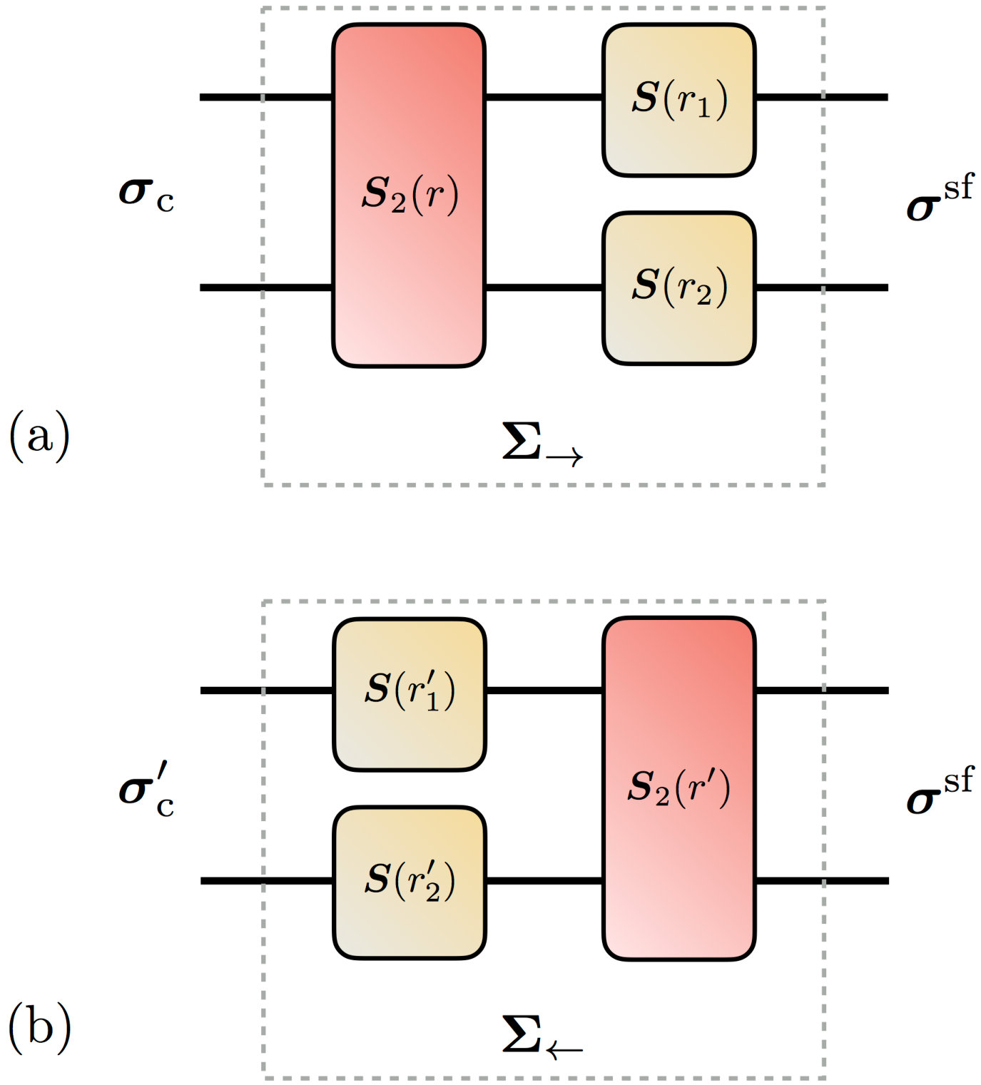 Figure 1
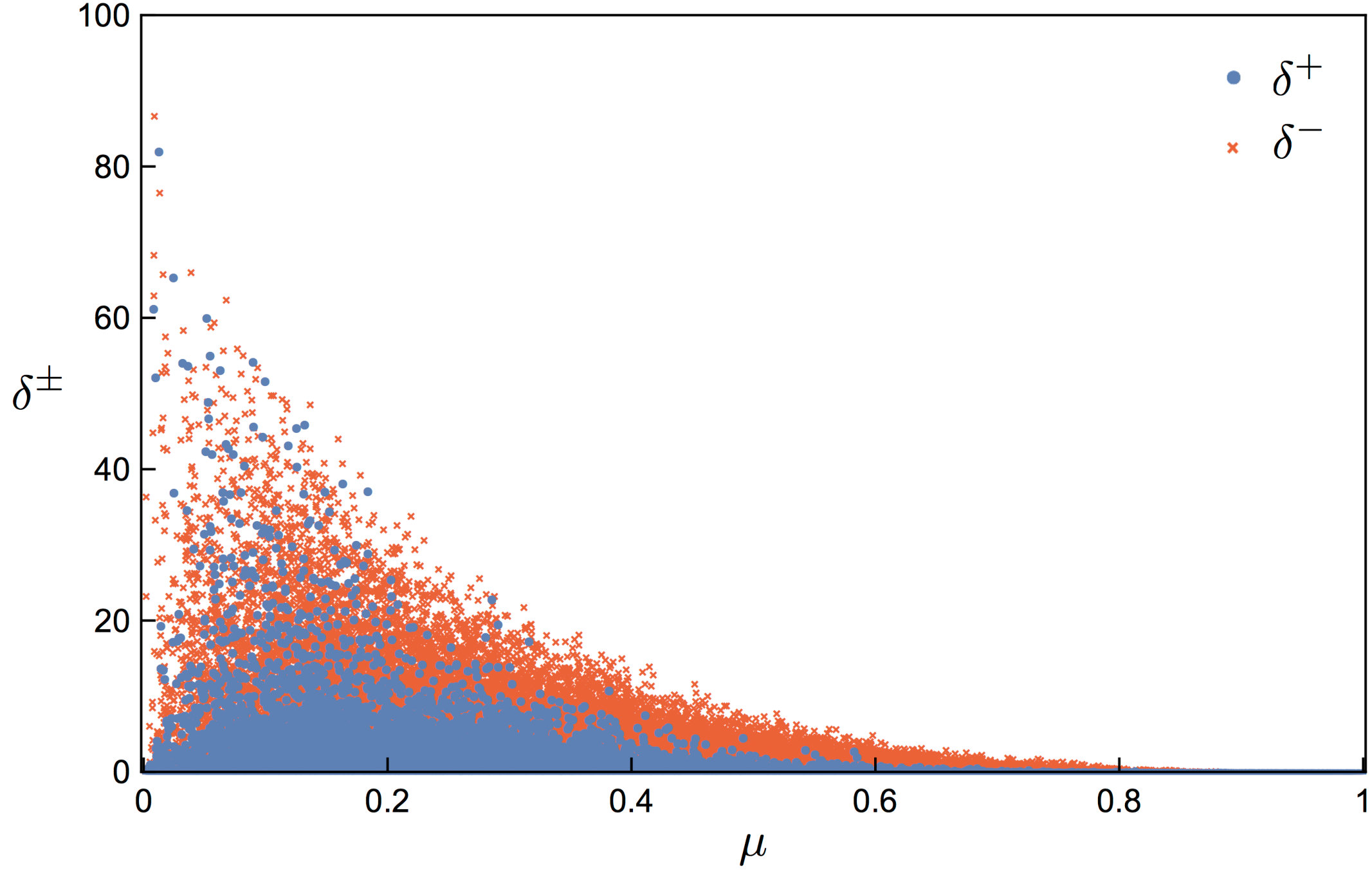 Figure 2
Peer Reviews
No public reviews on file for this paper yet. If you reviewed it on a platform where reviews are public (OpenReview, ICLR, NeurIPS, ICML), you can paste yours below so the community can read it here.
Videos
No videos yet. Explain this paper in a talk, walkthrough, or lecture? Add one.
Quantifying entanglement of formation for two-mode Gaussian states: Analytical expressions for upper and lower bounds and numerical estimation of its exact value
Spyros Tserkis
Centre for Quantum Computation and Communication Technology, School of Mathematics and Physics, University of Queensland, St Lucia, Queensland 4072, Australia
Sho Onoe
Centre for Quantum Computation and Communication Technology, School of Mathematics and Physics, University of Queensland, St Lucia, Queensland 4072, Australia
Timothy C. Ralph
Centre for Quantum Computation and Communication Technology, School of Mathematics and Physics, University of Queensland, St Lucia, Queensland 4072, Australia
Abstract
Entanglement of formation quantifies the entanglement of a state in terms of the entropy of entanglement of the least entangled pure state needed to prepare it. An analytical expression for this measure exists only for special cases, and finding a closed formula for an arbitrary state still remains an open problem. In this work we focus on two-mode Gaussian states, and we derive narrow upper and lower bounds for the measure that get tight for several special cases. Further, we show that the problem of calculating the actual value of the entanglement of formation for arbitrary two-mode Gaussian states reduces to a trivial single parameter optimization process, and we provide an efficient algorithm for the numerical calculation of the measure.
I Introduction
Quantifying entanglement is a non-trivial task, since various measures exist with different operational meanings, and most of them lack an analytical expression. Every entanglement measure needs to satisfy the following postulates Horodecki.et.al.RMP.09 ; Plenio.Virmani.B.14 : (i) vanishes on separable states, (ii) does not increase on average under local operations and classical communication (strong monotonicity), and, (iii) for pure states is equal to the entropy of entanglement, given by the von Neumann entropy of the reduced state.
Among several entanglement measures, entanglement of formation (EoF) is of significant importance, due to its well-defined physical meaning, i.e., EoF quantifies the entanglement of a state in terms of the entropy of entanglement of the least entangled pure state needed to prepare it Bennett.DiVincenzo.et.al.PRA.96 . For a given state \hat{\sigma}:=\sum_{i}p_{i}\mbox{|\psi_{i}\rangle}\mbox{\langle\psi_{i}|}, EoF is given by the convex-roof extension of the reduced von Neumann entropy of , i.e.,
[TABLE]
In general the calculation of EoF is NP-hard (non-deterministic polynomial-time hard) Huang.NJP.14 and there are only few cases, e.g., for qubits Wootters.PRL.98 , where Eq. (1) reduces to an analytical expression.
In this paper we work with systems of quantized radiation modes of the electromagnetic field that are described by continuous-variable states Serafini.B.17 ; Weedbrook.et.al.RVP.12 ; Adesso.Ragy.OSID.14 . Those modes are associated with the quadrature field operators and , where and are the annihilation and creation operators, respectively, with . We specifically focus on two-mode Gaussian states, which can be fully described by the first two statistical moments of the quadratures field operators.
In particular, we derive an upper bound for the entanglement of formation that comes as an extension of our recently derived lower bound for two-mode Gaussian states Tserkis.Ralph.PRA.17 . We also present a new optimization method for estimating the real value of the measure, supplemented by an explicit algorithm written in Mathematica for the numerical estimation of the measure supplementalmaterial . A numerical comparison of the lower and upper bounds to the exact value of the EoF is also presented for a set of randomly created states against their global purity.
In Sec. II we briefly review the structure of two-mode Gaussian states along with their classicality and separability conditions. In Sec. III we start by defining entanglement of formation, for the general case, and we continue by presenting the lower bound derived in Ref. Tserkis.Ralph.PRA.17 in order to use it for the derivation of the upper bound. We also introduce a new simple optimization method for the estimation of the real value of the measure for arbitrary states. Finally, we see how close the upper and lower bounds are to the actual EoF for randomly created entangled states. In Sec. IV we conclude our work.
II Gaussian states
II.1 State representation
A two-mode Gaussian state with zero mean value (for simplicity) can be fully described by its covariance matrix
[TABLE]
which is a real, symmetric, and positive definite matrix with elements proportional to the second-order moments of the quadrature field operators. The global purity of the state is given by , while local purities by and , respectively. In the standard form Duan.et.al.PRL.00 ; Simon.PRL.00 , the covariance matrix is given by , , with , and , with . The elements of the covariance matrix in the standard form can be parametrized over the local and global purities of the state as follows Adesso.Serafini.Illuminati.PRA.04
[TABLE]
where
[TABLE]
with , , , and (In Refs. Adesso.Serafini.Illuminati.PRA.04 ; Adesso.Illuminati.PRA.05 states with are called GMEMS and states with are called GLEMS). The parameters , , and are constrained as follows: , , and .
II.2 Classicality
Every quantum state can be represented in phase-space with the so-called -function Glauber.PR.63 ; Sudarshan.PRL.63 defined as
[TABLE]
where represents a coherent state and is a quasi-probability distribution. When the -function takes positive values it can be interpreted as a classical probability distribution and the corresponding state is called classical, and when the -function is negative or singular the corresponding state is called non-classical Mandel.PS.86 .
For two-mode Gaussian systems a state is classical if and only if , i.e., all the eigenvalues of its covariance matrix are greater or equal to 1 Serafini.B.17 .
II.3 State decomposition
According to Williamson’s theorem Williamson.AJM.36 , for every covariance matrix there is a symplectic transformation , such that
[TABLE]
with being the symplectic eigenvalues Vidal.Werner.PRA.02 , given by Serafini.Illuminati.DeSiena.JPB.04
[TABLE]
where is invariant under global symplectic operations. Re-arranging Eq. (8) we get
[TABLE]
where is a pure state, also called two-mode squeezed vacuum, that in the standard form is given by
[TABLE]
with , where , and is a positive semi-definite matrix. Equivalently, Eq. (8) can also be written as a symplectic transformation applied on a classical state , i.e.,
[TABLE]
Two decompositions relevant to our following analysis (graphically presented in Fig. 1) are the following
[TABLE]
and its transpose, i.e.,
[TABLE]
with , where is the local squeezing symplectic operation, i.e.,
[TABLE]
and is the two-mode squeezing symplectic operation given by
[TABLE]
II.4 Separability
Witnessing entanglement for arbitrary states is in general a difficult problem, however, in two-mode Gaussian states the separability criterion, also called the Peres-Horodecki criterion Peres.PRL.96 ; Horodecki.PLA.96 , is necessary and sufficient Duan.et.al.PRL.00 ; Werner.Wolf.PRL.01 ; Simon.PRL.00 . In particular, the separability of such states can be checked by the lowest symplectic eigenvalue of the partially transposed covariance matrix , i.e., separable states are the ones with Adesso.Serafini.Illuminati.PRA.04 , where
[TABLE]
with .
III Entanglement of Formation
Entanglement of formation (EoF) for a two-mode Gaussian state coincides with the Gaussian entanglement of formation (GEoF) Akbari-Kourbolagh.Alijanzadeh-Boura.QIP.15 and is equal to Wolf.et.al.PRA.04 ; Ivan.Simon.arXiv.08 ; Marian.Marian.PRL.08
[TABLE]
where is the entropy of entanglement of a pure state with a two-mode squeezing parameter , i.e., Holevo.Sohma.Hirota.PRA.99
[TABLE]
The optimal decomposition corresponds to the pure state (two-mode squeezed vacuum) with the least entropy of entanglement that can be transformed under local operations and classical communication into our state. From a resource theoretic point of view, the optimum decomposition corresponds to the minimum amount of two-mode squeezing needed for the creation of this pure state Tserkis.Ralph.PRA.17 .
The first attempt to derive a closed formula of this measure for mixed states was done by Giedke et.al. Giedke.et.al.PRL.03 in 2003, who gave an analytical expression of EoF for all symmetric states, i.e., . Two years later, Adesso et.al. Adesso.Illuminati.PRA.05 managed to give an analytical formula for GEoF (which was later shown to be equivalent with EoF) for all mixed states with , called GLEMS (), and for states with , also called GMEMS (). In order to calculate numerically the exact value of the measure, we can follow the approaches of either Wolf et.al. Wolf.et.al.PRA.04 , Marians Marian.Marian.PRL.08 or Ivan and Simon Ivan.Simon.arXiv.08 . Later in Sec. III we will show how we can simplify the numerical calculation and calculate the EoF with a trivial optimization over a single parameter.
Analytical lower bounds of the EoF have also been derived in Refs. Rigolin.Escobar.PRA.04 and Nicacio.Oliveira.PRA.14 . Finally, in 2017, a narrow lower bound was derived Tserkis.Ralph.PRA.17 , that is consistently closer to the actual value of the measure compared to the older ones, and has also the advantage of being tight for symmetric and states with .
III.1 Lower Bound for Entanglement of Formation
In Ref. Tserkis.Ralph.PRA.17 we derived a lower bound for the entanglement of formation. In this section we re-derive it in a more elegant and compact way.
Let us assume all the possible decompositions of a state
[TABLE]
Among all pure states that satisfy the above decomposition, one has the minimum entropy of entanglement, i.e., the optimum pure state . Using this optimal state, we are able to calculate the EoF of the state as follows
[TABLE]
Two (but not the only) ways to construct a pure state is by applying the symplectic transformations or onto a couple of vacua. For every two-mode squeezing parameter of the transformation there is a corresponding parameter of the transformation . It is easy to show that for any pure state (this can be easily seen from Eq. (33) since value is the global minimum of ). Thus the global minimums of the two-mode squeezing parameters and of those two decompositions have the following ordering
[TABLE]
The above equation essentially implies that the least amount of two-mode squeezing we need to apply to a state to make it separable is always less or equal to the least amount of two-mode squeezing we need to create it.
Assuming a state in the standard form , the lowest value of the two-mode squeezing corresponding to the symplectic transformation has been calculated in Ref. Tserkis.Ralph.PRA.17 , and is equal to
[TABLE]
where we have set and . Thus, for entangled states () substituting into the monotonic function given in Eq. (19) we get a lower bound for the EoF, i.e.,
[TABLE]
This lower bound is in general quite close to the actual value (see Fig. 2) and it becomes tight when the transformation that corresponds to the optimal decomposition of the state is equivalent to the . It is trivial to show that , which means that when the two single-mode squeezers of either transformation or are equal to each other, they can commute through the two-mode squeezer and thus . That is true for both symmetric states and states with Tserkis.Ralph.PRA.17 .
It is also worth mentioning that the single-mode squeezing parameters and can also be analytically calculated for a given value of two-mode squeezing , i.e.,
[TABLE]
with
[TABLE]
III.2 Upper Bound for Entanglement of Formation
By definition of the measure, the entropy of entanglement of every pure state that satisfies the decomposition of Eq. (20) constitutes an upper bound to the EoF. Every pure state created by the symplectic decomposition applied onto a couple of vacua, can also be created by the symplectic decomposition applied onto a couple of vacua.
Let us use as a reference the pure state prepared with the transformation , with two-mode squeezing , and single-mode squeezing parameters and . The equivalent pure state prepared with the transformation has two-mode squeezing equal to
[TABLE]
with
[TABLE]
Setting for entangled states (), and by substituting this value into Eq. (19) we get an upper bound for the entanglement of formation
[TABLE]
that is actually quite narrow to the real value (see Fig. 2). It is apparent that based on the way the upper and lower bound are connected, when the lower one gets tight the upper one gets tight as well (which happens for symmetric states and states with ). After numerical calculations it seems that the upper bound becomes tight also for the case of states with , if the condition is satisfied, but the general validity of this argument is only conjectured.
III.3 Estimating Entanglement of Formation
Finding an analytical expression for the exact value of the entanglement of formation is still considered an open problem. In this section we re-define EoF through a straightforward optimization process that involves the minimization over a single parameter.
As we discussed in the previous section, Eq. (35) is in general an upper bound for EoF, since any valid pure state of Eq. (20) has entropy of entanglement equal or greater to the optimal one. In order to find the optimal one we could minimize the upper bound over every possible pure state, however since we already have the squeezing values for the lower and upper bound we can express EoF as
[TABLE]
The problem of writing down Eq. (36) as a closed formula is that the function that needs to be optimized is in general non-smooth. As mentioned before, though, for the cases of symmetric states, i.e., , and states with , we don’t need to optimize Eq. (36), since we just have to set .
As we mentioned before, other methods of reaching the actual value for EoF have also been derived, but the one given in Eq. (36) is significantly easier for numerical calculations. A specific algorithm written in Mathematica has also been developed supplementalmaterial , that numerically evaluates the exact value of EoF for an arbitrary two-mode Gaussian state written in its standard form and parametrized according to Sec.II A.
It worths also comparing the upper and lower bound to the actual value of EoF in order to see how close they are. In Fig. 2, we randomly generate a large number of entangled states, and for each one we calculate the percentile relative difference, given by
[TABLE]
against the global purity of the corresponding state. As we clearly see for a random state the purity is inversely proportional to the relative difference between and . It is also apparent that the upper bound is on average closer to the exact value than the lower bound. Thus, besides the cases mentioned above, the upper and lower bounds can also be faithfully used for analytical calculations of the EoF for states with high purities, e.g., .
IV Conclusions
In conclusion, we derived an upper bound for the entanglement of formation for two-mode Gaussian states, that comes as an extension to the lower bound that we had recently derived in Ref. Tserkis.Ralph.PRA.17 . The two bounds become tight for a wide range of states but they can also be considered quite faithful for highly pure states. We introduced a new method for computing the actual value of the entanglement of formation for two-mode Gaussian states, based on an optimization process over a single parameter, and we also provided a code written in Mathematica for the numerical estimation of the measure for arbitrary two-mode Gaussian states supplementalmaterial .
V Acknowledgments
The research is supported by the Australian Research Council (ARC) under the Centre of Excellence for Quantum Computation and Communication Technology (CE170100012).
The reference list from the paper itself. Each links out to its DOI / PubMed record.
- 1(1) R. Horodecki, P. Horodecki, M. Horodecki & K. Horodecki Rev. Mod. Phys. 81, 865-942 (2009) .
- 2(2) M. B. Plenio & S. S. Virmani Quantum Information and Coherence, Ch. 8 (Springer, Switzerland, 2014).
- 3(3) C. H. Bennett, D. P. Di Vincenzo, J. A. Smolin & W. K. Wooters Phys. Rev. A 54, 3824 (1996) .
- 4(4) Y. Huang, New J. Phys. 16 , 033027 (2014) .
- 5(5) W. K. Wootters Phys. Rev. Lett. 80, 2245 (1998) .
- 6(6) A. Serafini, Quantum Continuous Variables: A Primer of Theoretical Methods , (CRC Press, 2017).
- 7(7) C. Weedbrook et al. , Rev. Mod. Phys. 84, 621-699 (2012) .
- 8(8) G. Adesso, S. Ragy, and A. R. Lee, Open Syst. Inf. Dyn. 21, 1440001 (2014) .