Determining the depth of Jupiter's Great Red Spot with Juno: a Slepian approach
Eli Galanti, Yohai Kaspi, Frederik J. Simons, Daniele Durante, Marzia, Parisi, and Scott J. Bolton

TL;DR
This paper introduces a novel Slepian function-based method to estimate the depth of Jupiter's Great Red Spot using gravity measurements from Juno, providing insights into its structure and the planet's atmospheric dynamics.
Contribution
It proposes a new approach combining gravity data and Slepian functions to determine the GRS depth, improving accuracy over previous methods.
Findings
Gravity signal detectable for GRS depths >300 km
Uncertainty of about ±100 km for 1000 km depth
Method effective with limited measurements
Abstract
One of Jupiter's most prominent atmospheric features, the Great Red Spot (GRS), has been observed for more than two centuries, yet little is known about its structure and dynamics below its observed cloud-level. While its anticyclonic vortex appearance suggests it might be a shallow weather-layer feature, the very long time span for which it was observed implies it is likely deeply rooted, otherwise it would have been sheared apart by Jupiter's turbulent atmosphere. Determining the GRS depth will shed light not only on the processes governing the GRS, but on the dynamics of Jupiter's atmosphere as a whole. The Juno mission single flyby over the GRS (PJ7) discovered using microwave radiometer measurements that the GRS is at least a couple hundred kilometers deep (Li et al. 2017). The next flybys over the GRS (PJ18 and PJ21), will allow high-precision gravity measurements that can be used…
Click any figure to enlarge with its caption.
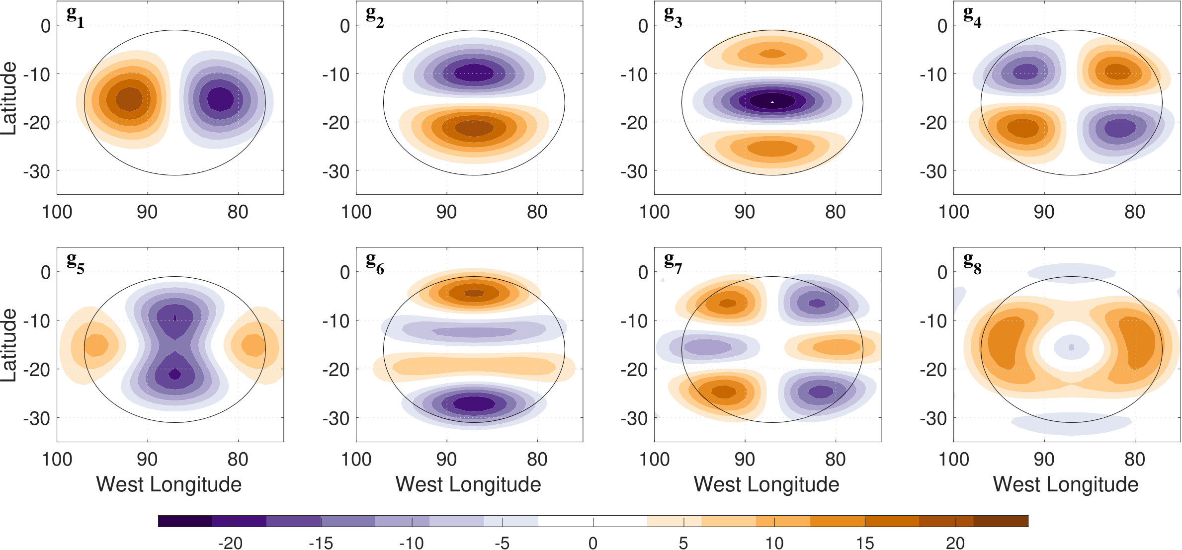 Figure 1
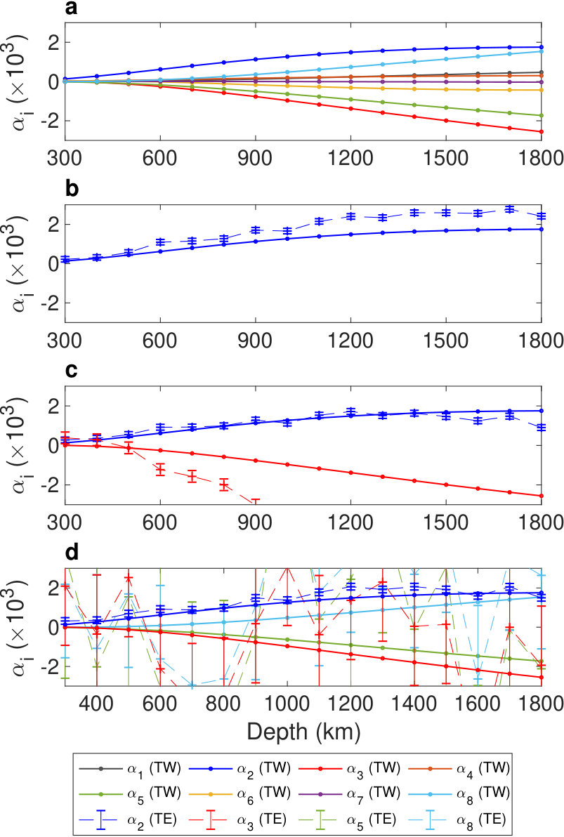 Figure 2
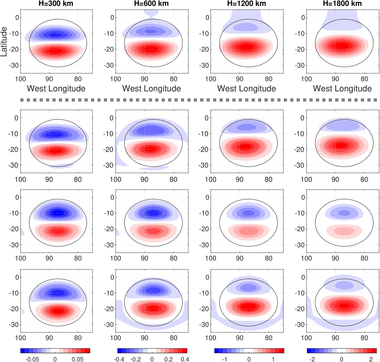 Figure 3
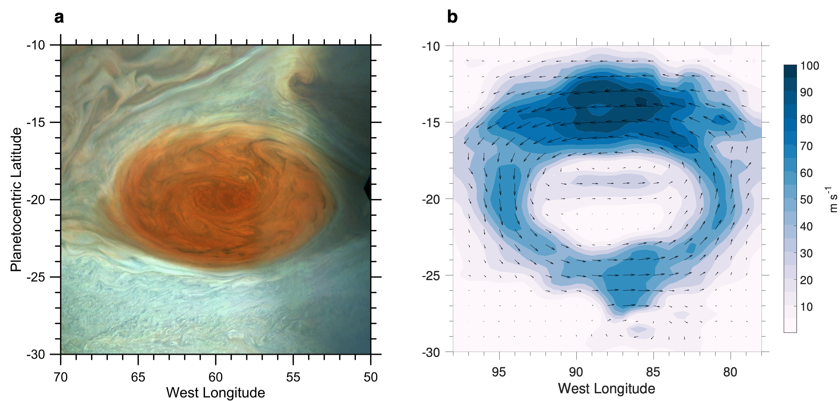 Figure 4
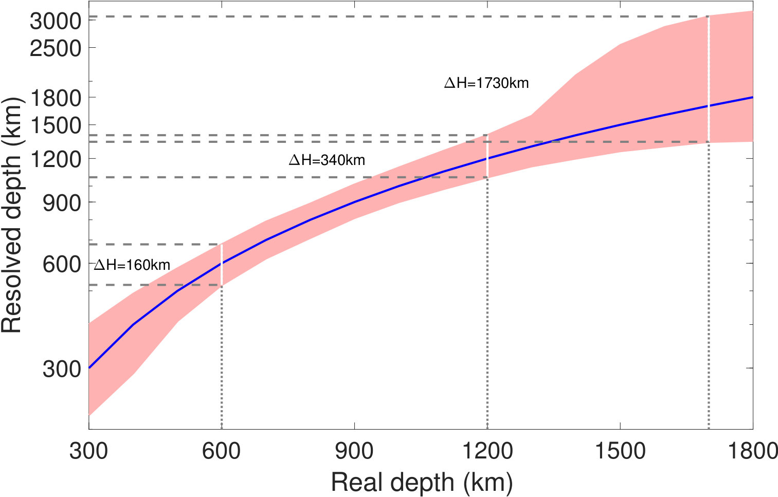 Figure 5
Peer Reviews
No public reviews on file for this paper yet. If you reviewed it on a platform where reviews are public (OpenReview, ICLR, NeurIPS, ICML), you can paste yours below so the community can read it here.
Videos
No videos yet. Explain this paper in a talk, walkthrough, or lecture? Add one.
Determining the depth of Jupiter’s Great Red Spot with Juno: a Slepian approach
Eli Galanti1, Yohai Kaspi1, Frederik J. Simons2, Daniele Durante3, Marzia Parisi4,
and Scott J. Bolton5
(Astrophysical Journal Letters, in press)
Abstract
One of Jupiter’s most prominent atmospheric features, the Great Red Spot (GRS), has been observed for more than two centuries, yet little is known about its structure and dynamics below its observed cloud-level. While its anticyclonic vortex appearance suggests it might be a shallow weather-layer feature, the very long time span for which it was observed implies it is likely deeply rooted, otherwise it would have been sheared apart by Jupiter’s turbulent atmosphere. Determining the GRS depth will shed light not only on the processes governing the GRS, but on the dynamics of Jupiter’s atmosphere as a whole. The Juno mission single flyby over the GRS (PJ7) discovered using microwave radiometer measurements that the GRS is at least a couple hundred kilometers deep (Li et al.,, 2017). The next flybys over the GRS (PJ18 and PJ21), will allow high-precision gravity measurements that can be used to estimate how deep the GRS winds penetrate below the cloud-level. Here we propose a novel method to determine the depth of the GRS based on the new gravity measurements and a Slepian function approach that enables an effective representation of the wind-induced spatially-confined gravity signal, and an efficient determination of the GRS depth given the limited measurements. We show that with this method the gravity signal of the GRS should be detectable for wind depths deeper than 300 kilometers, with reasonable uncertainties that depend on depth (e.g., 100 km for a GRS depth of 1000 km).
*1**Department of Earth and Planetary Sciences, Weizmann Institute of Science, Rehovot, Israel
2Department of Geosciences, Princeton University, New Jersey, USA
3Dipartimento di Ingegneria Meccanica e Aerospaziale, Sapienza Università di Roma, Rome, Italy
4Jet Propulsion Laboratory, California Institute of Technology, Pasadena, California , USA
5outhwest Research Institute, San Antonio, Texas , USA*
1 Introduction
Jupiter’s Great Red Spot (GRS) has been an iconic feature in the Solar System for centuries. Ever since it was discovered, hundreds of years ago, it perplexed astronomers with its shape, color and consistency. Nonetheless, little is known about the GRS, particularly about how deep into the gaseous planet this anticyclonic vortex extends. On the one hand, it resembles an Earth-like atmospheric vortex, suggesting it is driven by shallow atmospheric processes, and should be shallow and confined to some weather-layer (Dowling and Ingersoll,, 1988, 1989). On the other, its centuries-long existence within Jupiter’ ’s turbulent atmosphere indicates that it must contain significant mass otherwise it would have been sheared apart by the jets and other vortices. The depth to which it extends carries with it great implications on the mechanisms driving and maintaining it. Until recently, the depth of Jupiter’s atmosphere itself was unknown, but recent gravity measurements by the Juno spacecraft (Iess et al.,, 2018) allowed determining that the atmospheric jets on Jupiter extend down to depths of thousands of kilometers ( bars in pressure, Kaspi et al., 2018). The goal of this study is to propose a new methodology for interpreting the Juno gravity measurements in order to determine the depth of the GRS.
The Juno spacecraft orbits Jupiter every 53 days on a polar, highly eccentric orbit with perijove at 4000 km above Jupiter’s cloud-level (Bolton et al.,, 2017; Folkner et al.,, 2017). To allow a full coverage of the planet, every perijove is at a different longitude with a planned longitudinal separation of 11.25 degrees over the entire mission. As the GRS drifts by 110 degrees eastward every year (Simon et al.,, 2018) this provides, in principle, several opportunities for passes over the GRS. The first of these has been on orbit 7 (PJ7), but this orbit was devoted to microwave measurements, meaning radio science operated only in the X-band, thus preventing applying the plasma calibration scheme, which requires simultaneous Ka-band data (Iess et al.,, 2018). Orbits 18 (PJ18) and 21 (PJ21) will fly over the GRS in gravity mode, meaning they will operate with the more accurate Ka-band.
Differently than the depth estimate of the zonal jets, which is obtained using the zonal gravity harmonics, for the case of the GRS a non-zonal localized field is required. Parisi et al., (2016) used the tesseral gravity field to estimate the depth, and found that the GRS must be at least 2000 km deep in order to be detected. However, that estimate of the gravity signature required the determination of a large number of spherical harmonics, resulting in a considerable uncertainty in the solution. Here we propose a new approach, using Slepian functions that are designed specifically for isolated gravity measurements of local spatial features (e.g., Simons and Dahlen,, 2006; Simons et al.,, 2009; Harig and Simons,, 2012; Plattner and Simons,, 2017). We demonstrate its applicability to the GRS problem and examine the detectability of the GRS depth with the method, given the limited measurements expected.
2 Methods
2.1 Definition of Slepian functions
Given a phenomenon, such as the GRS winds and its accompanying gravity field, that is confined to a specific region, the Slepian functions form a basis set specifically to maximize the phenomenon representation inside the region, and minimize it outside the region. This is in contrast to the traditional spherical harmonics that are set to represent global signals with no preferences to specific regions. We follow here the derivation given by Simons et al., (2006), sections 3.3 and 4.1, for Slepian functions concentrated over an arbitrarily shaped region constructed from a band-limited set of spherical harmonic functions. Let , a real-valued function on a unit sphere, be given by a spherical harmonic expansion to bandwidth ,
[TABLE]
where and are the degree and order, and is the area of the sphere. Defining the spatial and spectral norms as
[TABLE]
where is the region of interest, the problem of maximizing the spatial concentration of becomes
[TABLE]
The ratio is a measure of the spatial concentration. Using Equations (1) and (2) this measure can be written as
[TABLE]
where
[TABLE]
The problem can now be formulated as an algebraic eigenvalue problem
[TABLE]
The solutions to this equation form the Slepian basis of concentrated functions in the region . Each solution is a vector including the amplitudes of each of the spherical harmonics used in the definition. The number of meaningful functions (that are well concentrated in the region of area ) depends on the bandwidth and the fractional area of the region of concentration, and can be calculated using the Shannon number
[TABLE]
where are the solutions to Equation (4).
We can now define the basis of Slepian functions for the region of interest. We define it as an ellipse centered at *∘E and ∘*S that spans 20 degrees in longitude and 30 degrees in latitude. This is similar in longitudinal range to the region of strong winds (Figure 1b), but is larger in latitudinal range and somewhat shifted northward to account for the actual gravity signal (discussed in section 3).
Equations (1)-(5) define the canonical Slepian functions of Simons et al., (2006), but here we restrict the range of all of the sums to only include harmonics with through and through . Furthermore, as the zonal harmonics ( for all ) are used in the Juno gravity analysis we exclude them from the Slepian functions. We also exclude all for through because the low degree tesseral field may be related to large scale structure and might be needed for the overall Juno analysis. This ensures that when incorporating the GRS Slepian functions in the Juno gravity analysis, there will be no ambiguity in the values of the spherical harmonics. Our Slepian functions are selectively band-passed rather than band-limited, and they remain mutually orthonormal as well as orthogonal to the spherical harmonics of the excluded degrees and orders, avoiding contamination with their previously determined coefficients. The calculated first 8 Slepian functions are shown in Figure 2, and with the Shannon number being we will use in the analysis the first 10 functions to reconstruct the GRS gravity field.
2.2 The GRS induced gravity signal
We define the flow structure involved in the GRS similarly to Parisi et al., (2016) and Galanti et al., 2017a to be
[TABLE]
where ] is the observed cloud-level wind (Figure 1b), projected along cylinders after its zonal mean is subtracted, km is the planet mean radius, and is the exponential decay scale of the cloud-level wind. Note that the exact nature of the decay function might change for the analysis of the actual measurements (e.g., Kaspi et al.,, 2018).
Due to the strong winds around the vortex the geostrophic gradient creates a density anomaly with respect to its surroundings, that can be calculated via thermal wind balance, namely
[TABLE]
where is the 3D velocity, is the planetary rotation rate, is the background density field, is the mean gravity vector and is the dynamical density anomaly (Pedlosky,, 1987; Kaspi et al.,, 2009). Other effects not included in this balance, such as the anomalous gravity and centrifugal forces induced by the density anomalies (Zhang et al.,, 2015; Cao and Stevenson,, 2017), were shown, for the large scale stronger zonal flows, to have a small effect on the gravity solutions (Galanti et al., 2017b, ; Kaspi et al.,, 2018). In the case of the GRS winds, where the zonally mean wind is excluded, this holds even more so as the induced density anomalies are local to the GRS region and the induced gravity anomalies are negligible. The balance also does not include the effect of the centrifugal force acting due to curvature of the flow (gradient flow, Holton, 2004). This effect implies, for the GRS winds, an increase of about 5% in the accompanying density anomalies.
The gravity signal at the surface of the planet resulting from the density perturbations can be calculated (Galanti et al., 2017a, ) either directly or using spherical harmonics coefficients
[TABLE]
[TABLE]
where and are the degree and order of the expansion, respectively. The spatially dependent gravity field in the radial direction is then
[TABLE]
2.3 Using Slepian functions to define the GRS gravity
Given a set of Slepian functions (Equation 4), expressed as a combination of spherical harmonics and , and a thermal wind solution for the GRS gravity signal defined by and (Equations 8 and 9), the combination of the Slepian functions that best describe the GRS gravity field can be found by minimizing
[TABLE]
where (the amplitude of the Slepian functions) are the parameters to be optimized. A solution for is found by solving
[TABLE]
where
[TABLE]
and
[TABLE]
Therefore, given a gravity field concentrated in the GRS region (expressed in terms of spherical harmonics coefficients ) that field can be represented by a set of Slepian functions weighted by the coefficients .
The Slepian functions are defined at the planet’s surface, but in practice they have to be projected upward to the location of the Juno trajectory, where the gravitational pull on the spacecraft is acting. Theoretically, this could lead to degradation in the orthogonality of the Slepian functions (Simons and Dahlen,, 2006; Plattner and Simons,, 2017). The degree of the degradation is a function of the ratio between the target altitude and the radius of the planet, as well as the number and complexity of the Slepian functions used. For the case of the Juno trajectory over the GRS the altitudes of relevance range are from around 4000 km at perijove to around 15,000 km. Only at the outer edge of this range is the uncertainty in the measurement expected to surpass the gravity signal generated even in cases of very deep winds. The projection of gravity signal resulting from both the TW solution and that reconstructed using the Slepian functions can be calculated by multiplying each coefficient , and , by the factor , where is the altitude to which the gravity field is projected and is the degree of the spherical harmonics. Performing this analysis for the range of wind depths discussed here shows that for all altitudes the orthogonality of the Slepian functions does not degrade substantially. In fact, the major error in estimating the GRS depth with the Slepian functions comes from the number of spherical harmonics used to define the GRS region, and of course the largest errors arise from the spatially limited Juno measurements.
2.4 Estimating the GRS depth with the trajectory estimation (TE) model
Juno’s radio-science instrumentation is capable of providing very accurate Doppler measurements, with accuracies as low as 10 micron/s, at an integration time of 60 seconds. The Doppler measurements are then analyzed with MONTE, JPL’s orbit determination code, to determine parameters of Juno’s dynamical model, such as Jupiter’s spherical harmonics or the Slepian coefficients (Evans et al.,, 2016).
To assess Juno’s sensitivity to the gravitational signal induced by the GRS, we simulate Juno’s gravity experiment up until the end of the mission. We include all the designed Juno’s gravity passes, with the inclusion of PJ7 (non gravity-dedicated). For the determination of the GRS gravity signal, the largest contribution comes from the passes which fly over the GRS, namely PJ7, and the gravity-dedicated PJ18 and PJ21. We include all the passes planned until the end of the mission because, in order to be able to determine the signal from the GRS, a good knowledge of the zonally-symmetric field is required. The inclusion of the Slepian functions within the orbit determination code is straightforward since each Slepian function is a known linear combination of spherical harmonics. Note that the partial derivative of the observables with respect to the Slepian coefficient is also a linear combination of the partial derivatives of the observables with respect to the spherical harmonics (Han,, 2008; Goossens et al.,, 2012).
The simulations have been performed by generating 1-day trajectories around Jupiter’s closest approach. Jupiter’s gravity field is assumed to be composed from a zonally symmetric field (following Iess et al., 2018) plus the addition of the signal of the GRS, for the different depths, represented with the Slepian functions.
3 Realizations of the GRS induced gravity field
The GRS is constantly moving in the zonal direction with respect to Jupiter system III with a rate of about (Simon et al.,, 2018), and therefore its longitudinal position has to be determined with respect to PJ18 and PJ21. Other changes to the GRS exists with time, such as its size and strength, but these should not change much within the time interval between the time in which the GRS shape is determined and the time of the gravity measurements. An example of the GRS, as observed recently in the cloud-level (Fig. 4 from Sanchez-Lavega et al.,, 2018), is shown in Figure 1a. The strongest winds are expected in the transition between the brown (belts) and white (zones) clouds.
The GRS-induced gravity signal is calculated as defined in Section 2.2, thus allowing the examination of the expected gravity signal under different scenarios of wind depths. The calculated gravity is shown in Figure 3 (top panels) for e-folding depths of 300, 600, 1200 and 1800 km. For shallow winds, the signal is mostly a dipole in the north-south direction with a negative patch north of the positive one. The dipole structure results from a combination of factors, coming from the product of the background density and the winds, on the of Equation 7, since the former increases with depth and the latter decreases with depth. As a result, the gradient in the direction of the axis of rotation gives positive values in the upper layers and negative values in the deeper layers, thus creating a dipole structure in the radial direction. However, because the winds extend inward in the direction of the axis of rotation (Equation 7), this vertical dipole is shifted such that the negative density anomalies in the deeper layers are seated northward of the positive density anomalies in the upper layers. This slantwise density dipole, when integrated (Equations 8,9), results in a north-south dipole in the gravity anomalies. For deeper winds, the positive part of the gravity dipole becomes stronger compared to the negative part, with a slight shift of the entire pattern to equatorward The weakening of the negative part of the dipole results from the negative density anomalies being pushed into deeper layers that have less effect on the surface gravity anomalies.
With the Slepian functions we can reconstruct the gravity field for the 4 wind depth cases (Figure 3, upper panels) using Equation (11). First, we reconstruct it with all 10 Slepian functions (Figure 3, second row panels). It is evident that most of the gravity signal is being reconstructed with these functions. The values calculated for the first 8 Slepian functions are shown in Figure 4a, for depth ranging from 300 to 1800 km. Several characteristics appear: first, there are 4 functions that determine most of the signal: . Second, for shallow flows the largest contribution comes from (blue), but for cases with winds deeper than 700 km other functions make a sizable contribution as well, mostly (red), (green), and (light blue). Given this behavior, we can reconstruct the gravity signal with a subset of the functions. In Figure 3 (third and forth rows) we show 2 cases
- using only, and using . As expected, using only results in a fairly good reconstruction for the shallower cases, while using the 4 leading Slepian functions results in a reconstruction that is very similar to the original signals.
4 The GRS detectability
We perform a theoretical examination of the method, using the planned trajectories of PJ18 and PJ21, similar to the analysis of Galanti et al., 2017a , where the wind-induced gravity field is used to simulate the Juno trajectories with the Trajectory Estimation (TE) model. Here, we use the wind-induced gravity signal in the GRS region (Figure 3) for a depth range of 300-1800 km to simulate the expected effect on the Juno trajectories PJ18 and PJ21. Then, given the modified Juno trajectory, we include the Slepian functions in the gravity analysis, to examine if the wind-induced values for the Slepian functions (Figure 4a) can be recovered.
Reconstructing with all 10 Slepian functions turns out to be not feasible since the uncertainties associated with the solution are much larger than the values themselves, due to large correlations, forcing a reduction in the number of functions to be used. Identifying the most important functions for the GRS gravity signal (largest values in Figure 4a) we can use only a subset of the functions in the estimation process. The largest contribution comes from , especially for the shallow cases, since using the TE model to fit the gravity field with only (Figure 4b, dashed) shows a fairly good fit for all cases with some overestimation for deep flows. Adding as a second parameter to the fit (Figure 4c, dashed) shifts to give very good values even for deep winds, but the value of cannot be recovered for winds deeper than 500 km. Finally, fitting with , , , and (Figure 4d, dashed) gives again a good estimate for , but the other 3 Slepian functions remain unresolved, suggesting that aside from the other Slepian functions are highly correlated in their manifestation in the Juno trajectory. Whether we fit the trajectory with only or together with , , and , it is possible to obtain a good estimation only for , the only parameter that can be used for determine the depth. The other Slepian functions can be used only to absorb other signals, preventing biases into . Note that the uncertainty on does not dramatically increase when including also the other Slepian functions.
We can now use these results to estimate the detectability of the GRS with the upcoming Juno overflights and the Slepian approach. Given that we are able to resolve we examine how the uncertainty associated with it is translated to an uncertainty in the estimated depth. For each depth , we take the TW value of plus the uncertainty given with the TE solution and search for depth at which the TW value matches the combined value, so that . The difference between the depths is taken as the upper uncertainty for the resolved depth. Similarly, we find using and . Note that as is not a linear function of . The resolved depths and the uncertainties associated with them are shown in Figure 5. For GRS depths of 300 to 1300 km the uncertainty is of the order of 100 km. For GRS depths larger than 1300 km, the lower uncertainty is similar but the upper uncertainty grows considerably, because the value grows slower at these depths. For example, if the winds are 1700 km deep, the lower uncertainty will be around 200 km but the upper uncertainty will be around 1500 km.
5 Conclusion
How deep is Jupiter’s Great Red Spot? Although it has been observed for a few centuries, little is known about its structure and dynamics below its observed cloud-level. The Juno mission will soon provide an opportunity to resolve this long standing question. The single Juno flyby over the GRS (PJ7) to date was dedicated to the microwave radiometer, which showed that it is at least a couple hundred kilometer deep (Li et al.,, 2017). The next flybys over the GRS, PJ18 and PJ21, to be carried during 2019, will allow high-precision gravity measurements that might be used to estimate how deep the GRS winds penetrate below the cloud-level. This however is a challenging task since the GRS is a small feature whose gravity signal is close to the detectability levels.
Here we propose a new method to determine the depth of the GRS using the upcoming gravity measurements, a dynamical flow model, and a Slepian functions approach that enables an effective representation of the wind-induced gravity signal, and an efficient determination of the GRS depth given the limited expected measurements.
We show that the gravity signal induced by the GRS winds can be well represented with a basis of Slepian functions, defined specifically for the GRS region. It is found that one function () dominates the signal for shallow cases, and for deeper winds additional 2-3 functions are needed (, and ), therefore only a few parameters are needed in order to resolve the gravity signal induced by the GRS and hence the depth of its winds.
Using the Juno trajectory estimation model we examine our ability to detect a range of wind depths. We find that for GRS wind depths of 300 to 1300 km the methodology allows to resolve the depth of the GRS winds with an accuracy of about 100 km. For GRS depths larger than 1300 km, the lower uncertainty is similar but the upper uncertainty grows considerably.
Acknowledgements: This research has been supported by the Israeli Ministry of Science, and the Helen Kimmel Center for Planetary Science at the Weizmann Institute of Science. DD was supported by the Italian Space Agency (ASI).
The reference list from the paper itself. Each links out to its DOI / PubMed record.
- 1Bolton et al., (2017) Bolton, S. J., Adriani, A., Adumitroaie, V., Allison, M., Anderson, J., Atreya, S., Bloxham, J., Brown, S., Connerney, J. E. P., De Jong, E., Folkner, W., Gautier, D., Grassi, D., Gulkis, S., Guillot, T., Hansen, C., Hubbard, W. B., Iess, L., Ingersoll, A., Janssen, M., Jorgensen, J., Kaspi, Y., Levin, S. M., Li, C., Lunine, J., Miguel, Y., Mura, A., Orton, G., Owen, T., Ravine, M., Smith, E., Steffes, P., Stone, E., Stevenson, D., Thorne, R., Waite, J., Durante, D., Ebe
- 2Cao and Stevenson, (2017) Cao, H. and Stevenson, D. J. (2017). Gravity and zonal flows of giant planets: From the euler equation to the thermal wind equation. J. Geophys. Res. (Planets) , 122:1–15.
- 3Choi and Showman, (2011) Choi, D. S. and Showman, A. P. (2011). Power spectral analysis of Jupiter’s clouds and kinetic energy from Cassini. Icarus , 216:597–609.
- 4Dowling and Ingersoll, (1988) Dowling, T. E. and Ingersoll, A. P. (1988). Potential vorticity and layer thickness variations in the flow around Jupiter’s great red spot and white oval BC. J. Atmos. Sci. , 45(8):1380–1396.
- 5Dowling and Ingersoll, (1989) Dowling, T. E. and Ingersoll, A. P. (1989). Jupiter’s Great Red Spot as a shallow water system. J. Atmos. Sci. , 46(21):3256–3278.
- 6Evans et al., (2016) Evans, S., Taber, W., Drain, T., Smith, J., Wu, H. C., Guevara, M., Sunseri, R., and Evans, J. (2016). MONTE: The Next Generation of Mission Design and Navigation Software. In 6th International Conference on Astrodynamics Tools and Techniques (ICATT) .
- 7Folkner et al., (2017) Folkner, W. M., Iess, L., Anderson, J. D., Asmar, S. W., Buccino, D. R., Durante, D., Feldman, M., Gomez Casajus, L., Gregnanin, M., Milani, A., Parisi, M., Park, R. S., Serra, D., Tommei, G., Tortora, P., Zannoni, M., Bolton, S. J., Connerney, J. E. P., and Levin, S. M. (2017). Jupiter gravity field estimated from the first two Juno orbits. Geophys. Res. Lett. , 44(10):4694–4700.
- 8(8) Galanti, E., Durante, D., Finochiaro, S., Iess, L., and Kaspi, Y. (2017 a). Estimating Jupiter gravity field using Juno measurements, trajectory estimation analysis, and a flow model optimization. Astronomical J. , 154(1).