Equivalence of Two Methods to Solve Static Electromagnetic Potentials
Weiwei Zhao, Hao Jin, Hao Guo

TL;DR
This paper proves the mathematical equivalence between solving Poisson's equation and directly integrating charge or current distributions to find static electromagnetic potentials, with examples confirming the results.
Contribution
It establishes the formal mathematical equivalence between two common methods for calculating static electromagnetic potentials.
Findings
Proves the equivalence mathematically
Provides explicit examples confirming the equivalence
Clarifies the relationship between two formalisms in electromagnetism
Abstract
In electromagnetic statics, the standard procedure to determine the electric scalar potential or magnetic vector potential in a bounded space is to solve Poisson's equation subject to certain boundary conditions. On the other hand, as a direct generalization of Coulomb's law or Biot-Savart law, the static electromagnetic potentials may also be obtained by directly integrating the electric charge or current distributions over the region (either volume or surface) where they are spread out. What is the relation between these two formalisms? In this article, we prove that they are in fact equivalent to each other in mathematics. Examples are also presented to explicitly show the validity of this equivalence.
Click any figure to enlarge with its caption.
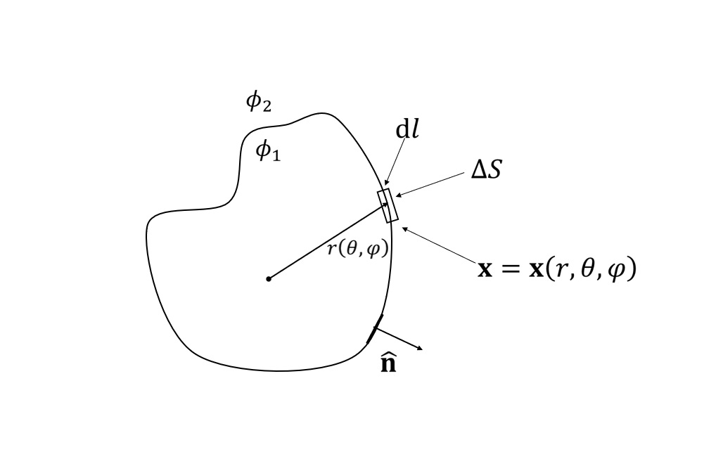 Figure 1
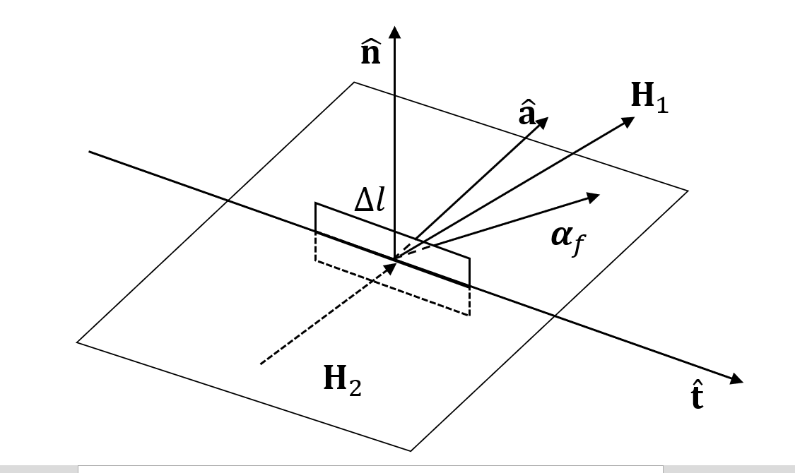 Figure 2
Peer Reviews
No public reviews on file for this paper yet. If you reviewed it on a platform where reviews are public (OpenReview, ICLR, NeurIPS, ICML), you can paste yours below so the community can read it here.
Videos
No videos yet. Explain this paper in a talk, walkthrough, or lecture? Add one.
Taxonomy
TopicsQuantum and Classical Electrodynamics · Scientific Research and Discoveries · Electric Power Systems and Control
Equivalence of Two Methods to Solve Static Electromagnetic Potentials
Weiwei Zhao
Department of Physics, Southeast University, Nanjing 211189, China
Hao Jin
Department of Physics, Southeast University, Nanjing 211189, China
Hao Guo
Department of Physics, Southeast University, Nanjing 211189, China
Abstract
In electromagnetic statics, the standard procedure to determine the electric scalar potential or magnetic vector potential in a bounded space is to solve Poisson’s equation subject to certain boundary conditions. On the other hand, as a direct generalization of Coulomb’s law or Biot-Savart law, the static electromagnetic potentials may also be obtained by directly integrating the electric charge or current distributions over the region (either volume or surface) where they are spread out. What is the relation between these two formalisms? In this article, we prove that they are in fact equivalent to each other in mathematics. Examples are also presented to explicitly show the validity of this equivalence.
I Introduction
In the theory of electrostatics, Coulomb’s law indicates that the electric potential in free space can be determined up to a constant provided the charge distribution
[TABLE]
where ( ) is the field (source) point, and is the dielectric constant. By applying the fact , it can be shown that Eq.(1) is the solution to Poisson’s equation
[TABLE]
Several preconditions are needed to justify the above result: There is only one kind of material (including the vacuum) of permittivity filling in the whole space, and the electric charge density is well behaved. In the realistic world, there exist various materials which have various shapes of boundaries. The find the electric potential, the routine method is to solve Poisson’s equation (2) in confined spaces with respect to certain boundary conditions, which is discussed in any text book on electrodynamics.
If a boundary is electrically charged, the surface charge density, which can be thought of as a special type of volume charge density singular at the boundary, must enter into the boundary conditions. Mathematically, the surface charge density can be expressed as where is a point at the boundary surface . Substitute this into Eq.(1), we get
[TABLE]
Here we emphasize that this is valid only when the materials on two sides of are the same, otherwise is not continuous when crossing . Note Eq.(I) represents the contribution of surface charges to the electric potential. In the routine method by solving Poisson’s equation, such kind of contribution is included by boundary effects (conditions). Thus, they are two parallel ways to solve the electric potential, and must be equivalent to each other as required by the uniqueness theorem. In fact, the expression (I) has already appeared in many text booksGriffiths (1999); Jackson (1999); Schwinger et al. (1998); Westgard (1996); Greiner (1998); Ohanian (1988); Schwartz (1987); Landau and Lifshitz (1984); Muller-Kirsten (2004); Wen (2010); Guo (2008); Zhao (2016). But a rigorous proof to show its equivalence to the method of solving Poisson’s equation is still missing. In the next section, we will present such a proof in mathematics. A parallel discussion to the magnetostatic potential will also be addressed.
II Proof of Equivalence
II.1 Electrostatic Field
For convenience, we refer the method by solving Poisson’s equation as the routine method. The second method is to sum all contributions to the electric potential produced by both volume (Eq.(1)) and surface (Eq.(I)) charge densities, and we refer it as the integral method. Without loss of generality, we consider a simple space configuration where there exists only one closed boundary that separates the space into two parts, labelled by 1 (inside) and 2 (outside) respectively. Let the volume charge density be unitedly described by . By the routine method, the electric potential is obtained via solving Poisson’s equation
[TABLE]
under the boundary condition
[TABLE]
Here is the normal vector of , pointing from region 1 to region 2. To solve this boundary value problem, we expand by a complete and orthogonal set of functions, usually the solutions of the associated Laplace’s equation . Next, by applying boundary conditions, the coefficients of each term in the linear expansion can be determined. In this way, the electric potential is fully solved.
By the integral method, the electric potential in each region can be uniformly expressed as
[TABLE]
if all kinds of charge distributions are given. To show the equivalence of the two methods, we only need to verify that Eq.(9) is indeed the solution to Eqs.(6), (7) and (8). The uniqueness theorem then guarantees that it is the only solution. We first prove this for generic situations, then give a more pedagogical discussion for the special case where is a spherical surface.
Proof:
The Poisson’s equation (6) is satisfied by plugging in Eq.(9)
[TABLE]
Here the surface integral vanishes since . The boundary is illustrated in Fig.1. In spherical coordinates, a point on is denoted by , where and and are the polar and azimuthal angles. The surface can be simply represented by , i.e. is a function of and . The first boundary condition, the continuity of across , seems quite apparent since the electric potentials in region 1, 2 are both expressed by Eq.(I). However, since it includes a surface integral (obviously we don’t need to worry about the volume integral), it is safe to check whether this term breaks the continuity or not. Assuming the origin of the coordinate system is inside the boundary (see Fig.1), a point with ( is a small positive number) is close to the outer/inner boundary. Expanding by Lengdre polynomials
[TABLE]
where is the angle between and , we get
[TABLE]
As , the condition \phi_{1}\big{|}_{S^{\prime}}-\phi_{2}\big{|}_{S^{\prime}}=0 is recovered.
To verify the condition (8), we choose a thin Gaussian pillbox covering a tiny patch of , as shown in Fig.1. We assume that the center of the pillbox is located at , and its thickness is . Thus, the top/bottom of the pillbox is represented by , of which the area is . Multiply the left-hand-side of Eq.(8) by and use Gauss’s theorem, we get
[TABLE]
where is the electric displacement vector, is the boundary of the pillbox, and the fact has been applied in the sixth line. Now plugging in Eq.(9) into Eq.(13), the first term does not contribute since must vanish outside the boundary (it represents the volume charge distribution), and the second term leads to
[TABLE]
Here is replaced by since it measures the change of , and is replaced by since is now at . Next, substitute the spherical-coordinate-expression of
[TABLE]
we get
[TABLE]
which finally leads to
[TABLE]
Hence, the two methods are indeed equivalent.
If is a geometrically regular boundary, the proof may be more perceivable. For simplicity, we only care about the condition (8). Assuming is a spherical surface of radius , the expansion (11) is now expressed as
[TABLE]
Substituting this into Eq.(9), and applying the addition formula of the spherical harmonics
[TABLE]
the left-hand-side of Eq.(8) becomes
[TABLE]
where is the -th coefficient of the series when is expanded by spherical harmonics.
In some situations, the integral expression (9) provides a more straightforward way to calculate the electrostatic field if the charge distribution is known. We will make a direct comparison by an explicit example in our later discussions.
II.2 Magnetostatic Field
A parallel theorem can be deduced in magnetostatics. In the standard routine, the magnetostatic potential is determined by solving Poisson’s equation
[TABLE]
with respect to the boundary conditions
[TABLE]
where is the surface current density. Similarly, the magnetic vector potential can also be obtained from a generalization to Biot-Savart law
[TABLE]
where the second integral is implied by applying , just as the evaluation in Eq.(I). The uniqueness theorem requires that this is a solution to the boundary value problem specified by Eqs.(23) and (24). Once again we emphasize that this theorem only applies to the situation that there exists only one type of material.
Proof:
Similar to Eq.(10), Eq.(25) is the solution to Poisson’s equation (23). For boundary conditions, we consider an Amperian loop as shown in Fig.2, of which the length and width are and such that (For end points inside/outside the boundary, the distance between them and the origin are denoted by / with ). Let be the tangent direction along the length side, and the normal direction of boundary. Define , indicating the normal direction of the Amperian rectangle. Note is stationery, then satisfies the Coulomb gauge condition . Applying Stokes’s theorem to evaluate the contour integral of along the Amperian rectangle, we have
[TABLE]
where the expression (25) has been plugged in. Here is the area surrounded by the Amperian loop
[TABLE]
and since is the normal vector of the infinitesimal patch . Similar to the electric part, the boundary is parameterized by , then . Applying Eqs.(27) and (15), Eq.(II.2) further yields
[TABLE]
Here the coordinate set denotes a point in , and the delta functions also force it to lie at the boundary . In other words, it is at the intersecting line between and . Next, applying , we get
[TABLE]
Note the contour integral of can also be evaluated as
[TABLE]
the arbitrariness of leads to
[TABLE]
Therefore, the solution (25) indeed satisfies the boundary condition. The continuity of across the surface can be simply verified in the same way as that of , and we omit the details here.
III Examples
As a comparison between the two methods, we use two examples to show their equivalence.
Example.1. Assume the surface charge density on a thin dielectric sphere of radius is maintained as , find the electrical potentials inside and outside the sphere.
Solution:
Routine Method:
The electric potentials inside and outside the boundary can be respectively expressed as
[TABLE]
Applying the boundary conditions, we get
[TABLE]
Note , we have
[TABLE]
We finally get
[TABLE]
Integral Method:
Applying Eq.(9), we get
[TABLE]
where denotes a point on the sphere, and . Let the angle between and be . Using the expression (21), the electric potential inside the sphere is
[TABLE]
Next, plug in the expression
[TABLE]
and evaluate the integral over , only the term is non-zero. Hence we have
[TABLE]
where we have applied the orthogonality relation
[TABLE]
In exactly the same way, the electric potential outside the sphere is given by
[TABLE]
The result agrees with that obtained by the routine method.
To explicit show the equivalence theorem in magnetostatics, we choose an example in Griffiths’s bookGriffiths (1999).
Example.2. A spherical thin shell, of radius , carrying a uniform surface charge , is set spinning at the angular velocity . Find the magnetic field inside and outside the sphere.
Solution:
Routine Method:
We can first solve Eq.(23) for subject to the boundary conditions (24), and then the magnetic field is obtained via . However, this will be very tedious since at least six sets of coefficients are needed to specify inside and outside the spherical shell due to the fact that is a vector field. A simpler and equivalent method is to introduce the magnetic scalar potential Guo (2008); Zhao (2016), satisfying the Laplace’s equation inside and outside the sphere since the electric current is only distributed on the spherical shell. The boundary condition is given by
[TABLE]
where is the radial component of , and is the surface electric current. Note , the boundary conditions for the magnetic scalar potential are then given by
[TABLE]
The general solution can be expressed as
[TABLE]
Substituting them into the boundary conditions, we get
[TABLE]
Hence the magnetic scalar potential is given by
[TABLE]
and the magnetic field is
[TABLE]
Integral Method:
Let the coordinate of a field point be , and the coordinate of a point at the spherical shell be . The magnetic vector potential is then given by
[TABLE]
Note the axis also depends on the position
[TABLE]
This contributes to the integration too. Expanding by Legendre polynomials, we have
[TABLE]
where is the angle between and . Next, by expanding by spherical harmonics and using Eq.(III), the integral in Eq.(53) is evaluated as
[TABLE]
where we have applied the relation in the second line, and the relation in the last line. Furthermore, by using the identity we get
[TABLE]
Substitute this into Eq.(III), we have
[TABLE]
Finally we get
[TABLE]
The corresponding magnetic field is
[TABLE]
which exactly agrees with Eq.(48).
IV Conclusion
We have discussed the integral expressions of the static electromagnetic potentials as a generalization to Coulomb’s law/Biot-Savart law when there exist surface charge/current distributions in some situation. We proved that it is equivalent to solve Poisson’s equations subject to certain boundary conditions. Explicit examples are also provided to show the applications of such integral expressions.
H. G. was supported by Teaching Research Foundation of Southeast University (Grant No. 5207022106A) and the National Natural Science Foundation of China (Grant No. 12074064).
The reference list from the paper itself. Each links out to its DOI / PubMed record.
- 1Griffiths (1999) D. J. Griffiths, Introduction to Electrodynamics (Prentice Hall, New Jersey, 1999).
- 2Jackson (1999) J. D. Jackson, Classical Electrodynamics (Wiley, New York, 1999).
- 3Schwinger et al. (1998) J. Schwinger, L. L. Deraad Jr., K. A. Milton, and W.-y. Tsai, Classical Electrodynamics (Westview Press, 1998).
- 4Westgard (1996) J. B. Westgard, Electrodynamics: A Concise Introduction (Springer-Verlag, New York, 1996).
- 5Greiner (1998) W. Greiner, Classical Electrodynamics (Springer, 1998).
- 6Ohanian (1988) H. C. Ohanian, Classical Electrodynamics (Prentice Hall, 1988).
- 7Schwartz (1987) M. Schwartz, Principles of electrodynamics (Dover Publications, New York, 1987).
- 8Landau and Lifshitz (1984) L. D. Landau and E. M. Lifshitz, Electrodynamics of Continuous Media (Pergamon, 1984).