The Metal-Rich Atmosphere of the Neptune HAT-P-26b
Ryan J. MacDonald, Nikku Madhusudhan

TL;DR
This study provides a detailed atmospheric analysis of exo-Neptune HAT-P-26b, revealing a metal-rich atmosphere with specific water and metal abundances, and predicts JWST observations will refine these measurements further.
Contribution
It offers the most precise exo-Neptune metallicity measurement to date and identifies potential metal hydrides, advancing understanding of exoplanet formation and atmospheric composition.
Findings
Atmosphere contains ~1.5% H2O and has super-solar metallicity.
Evidence for metal hydrides like TiH, CrH, or ScH at 4.1σ confidence.
JWST can significantly improve detection and measurement precision.
Abstract
Transmission spectroscopy is enabling precise measurements of atmospheric H2O abundances for numerous giant exoplanets. For hot Jupiters, relating H2O abundances to metallicities provides a powerful probe of their formation conditions. However, metallicity measurements for Neptune-mass exoplanets are only now becoming viable. Exo-Neptunes are expected to possess super-solar metallicities from accretion of H2O-rich and solid-rich planetesimals. However, initial investigations into the exo-Neptune HAT-P-26b suggested a significantly lower metallicity than predicted by the core-accretion theory of planetary formation and solar system expectations from Uranus and Neptune. Here, we report an extensive atmospheric retrieval analysis of HAT-P-26b, combining all available observations, to reveal its composition, temperature structure, and cloud properties. Our analysis reveals an atmosphere…
Click any figure to enlarge with its caption.
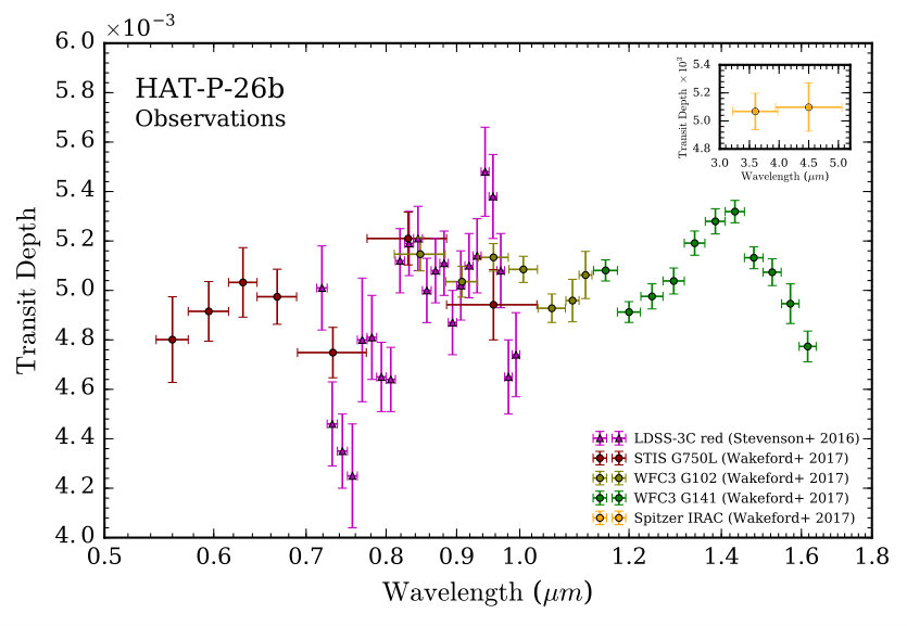 Figure 1
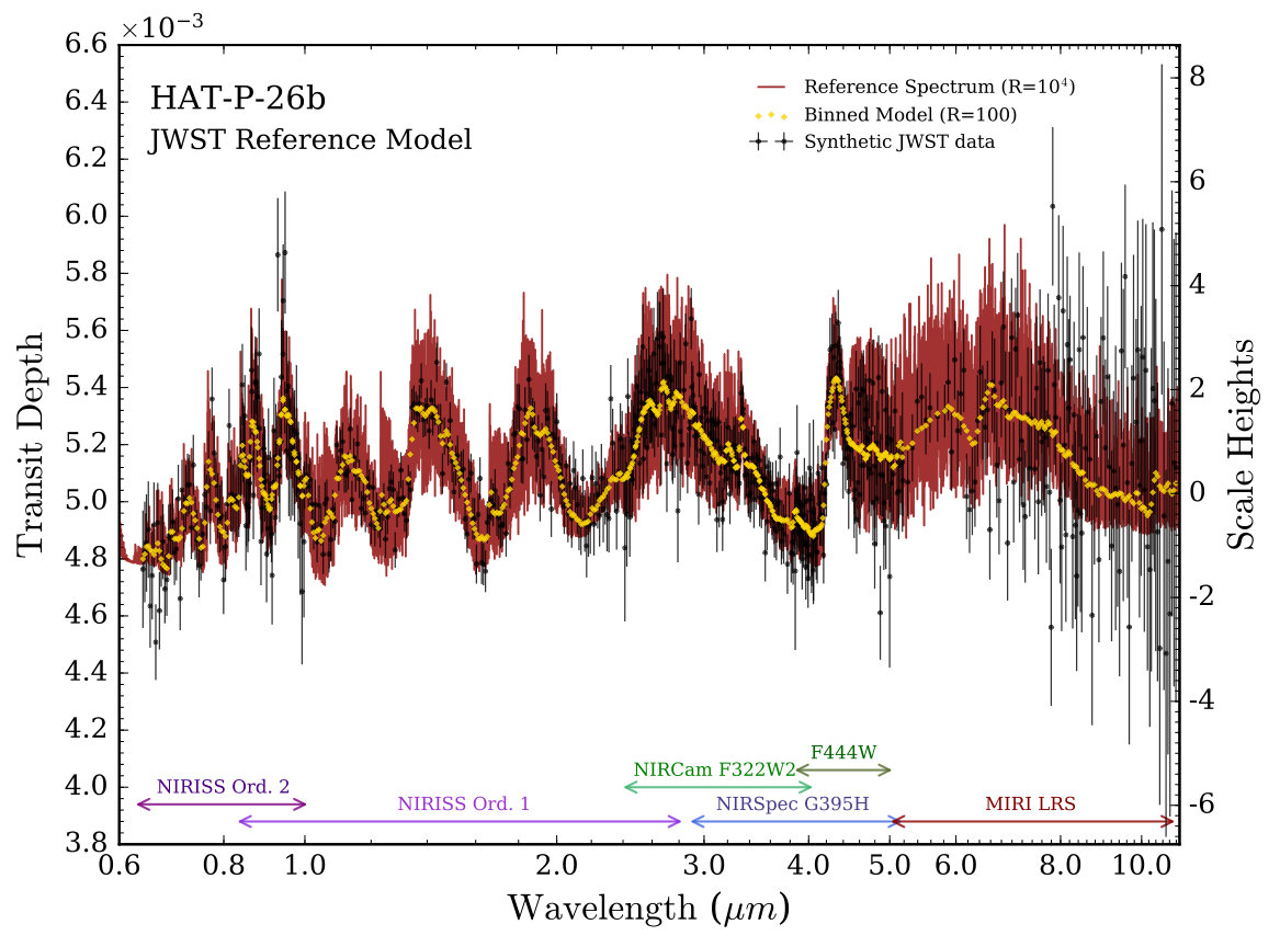 Figure 10
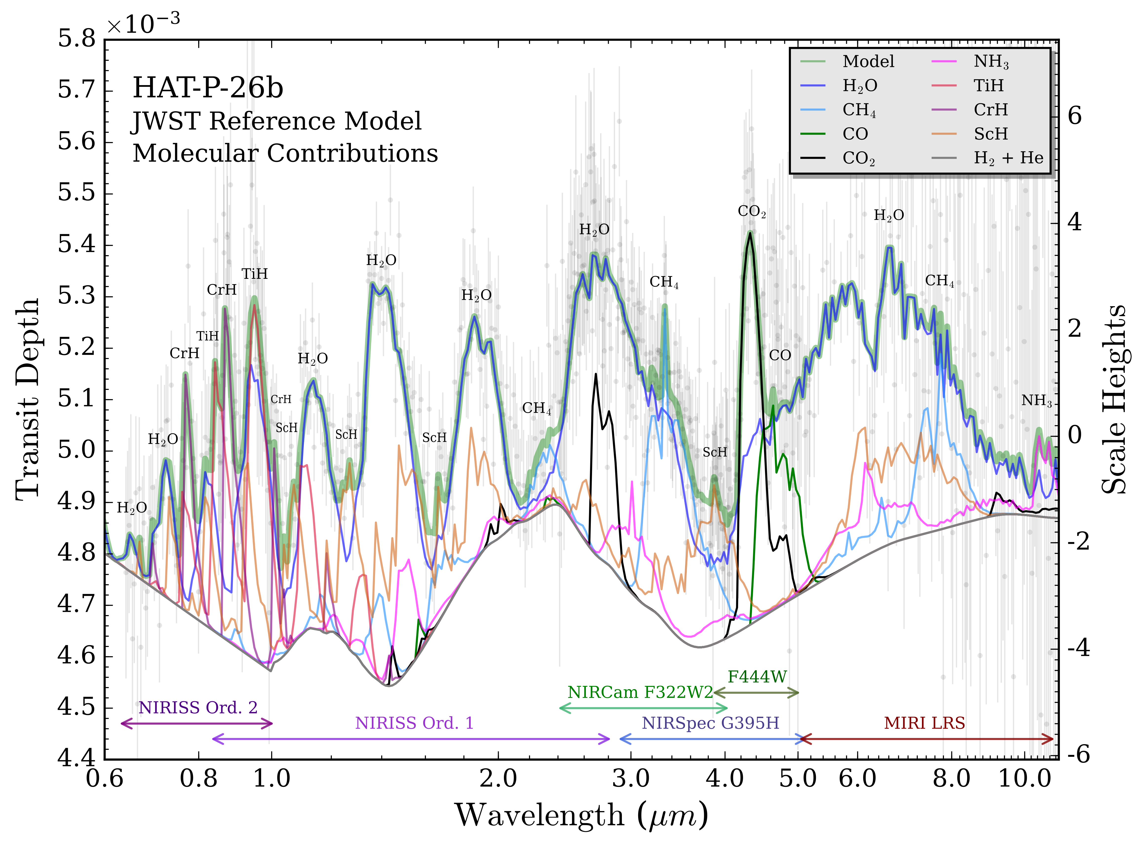 Figure 11
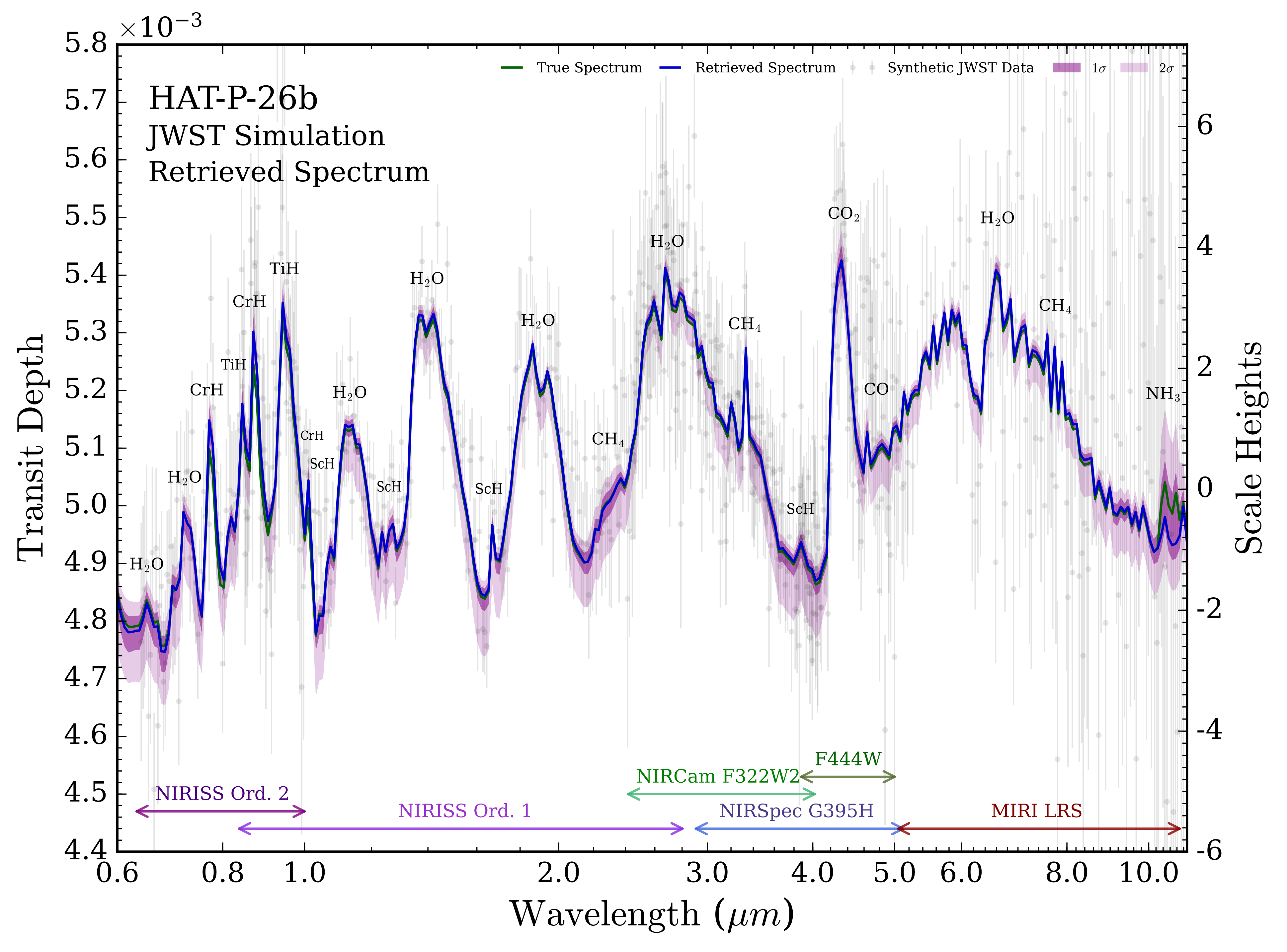 Figure 12
 Figure 13
 Figure 14
 Figure 15
 Figure 16
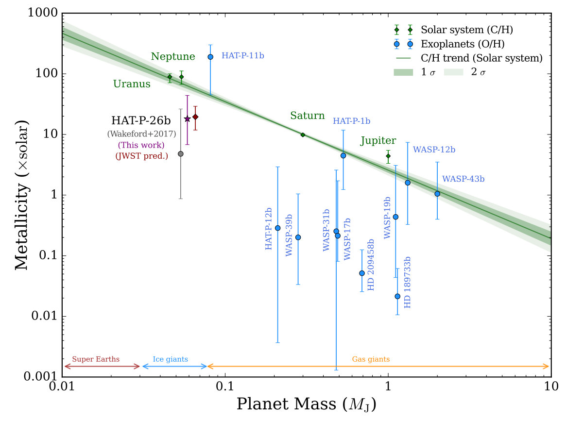 Figure 17
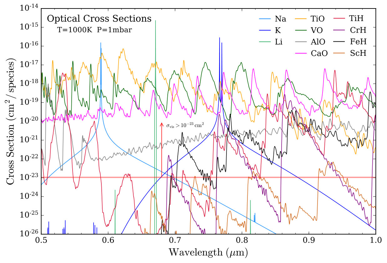 Figure 2
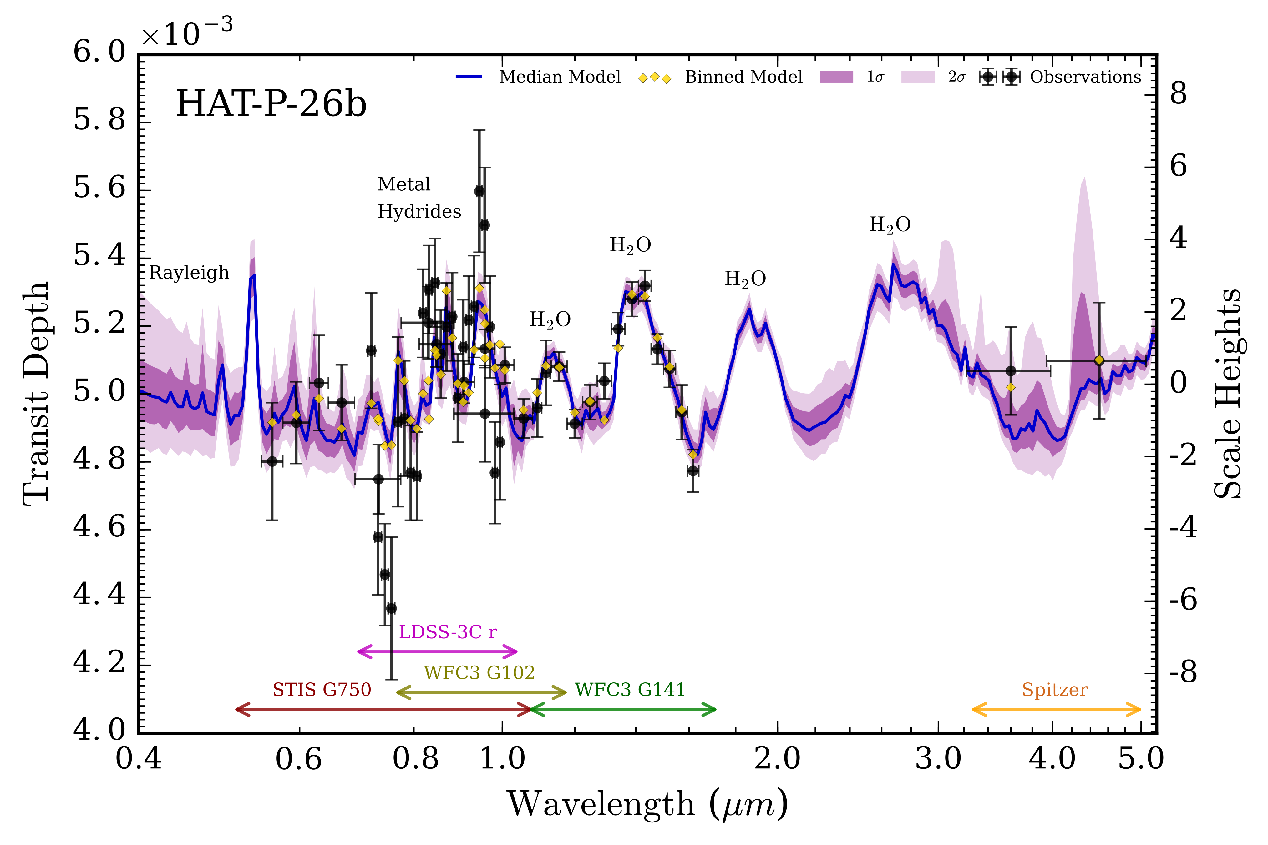 Figure 3
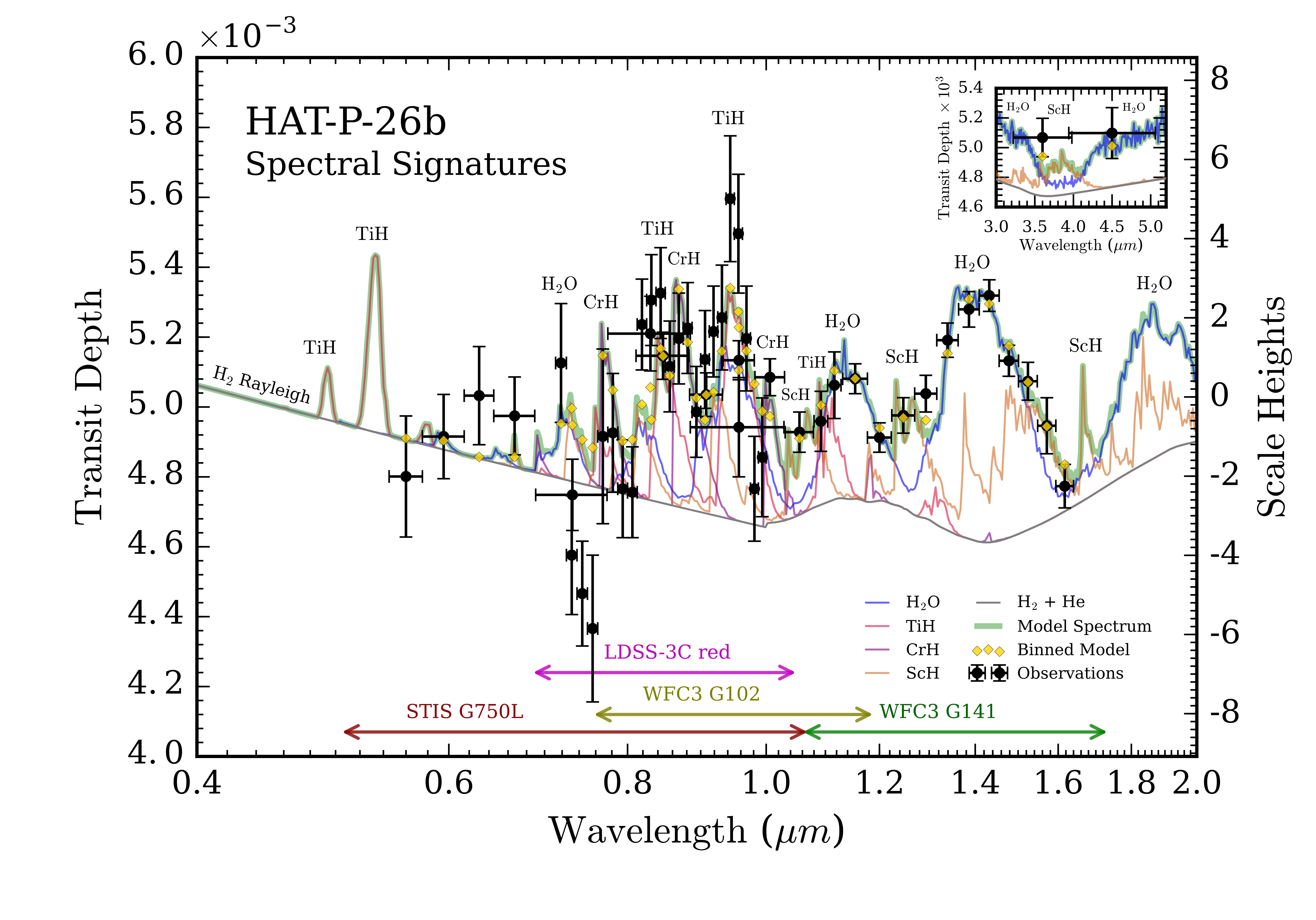 Figure 4
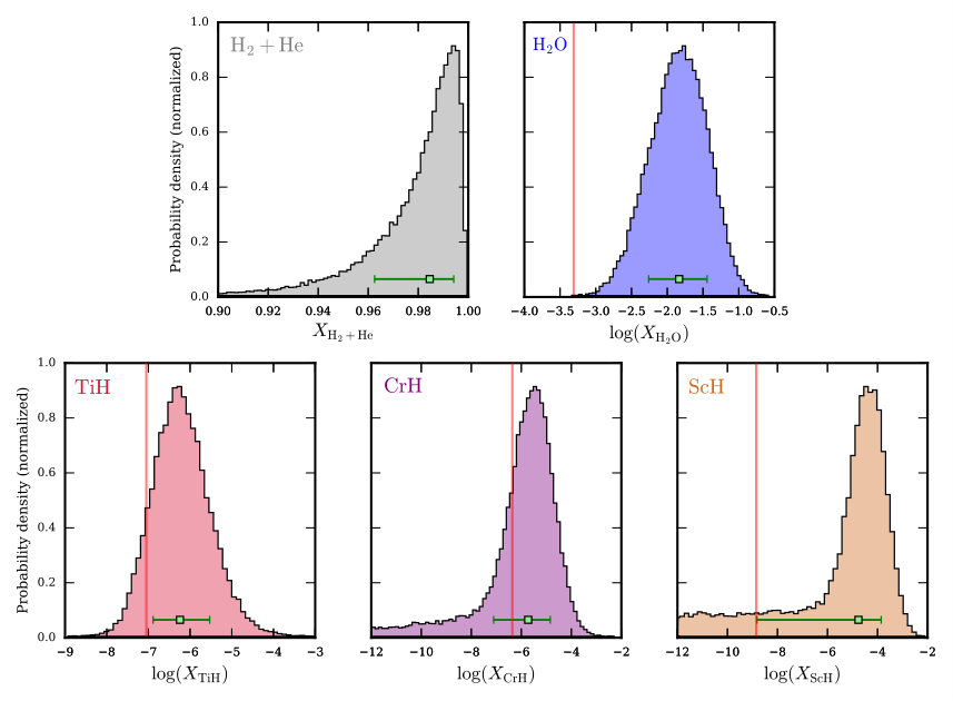 Figure 5
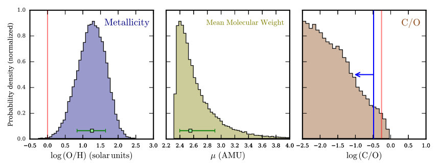 Figure 6
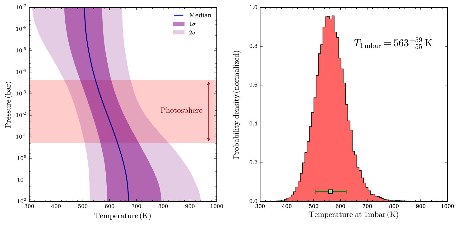 Figure 7
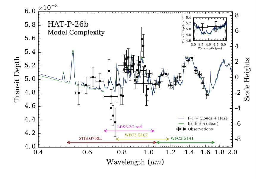 Figure 8
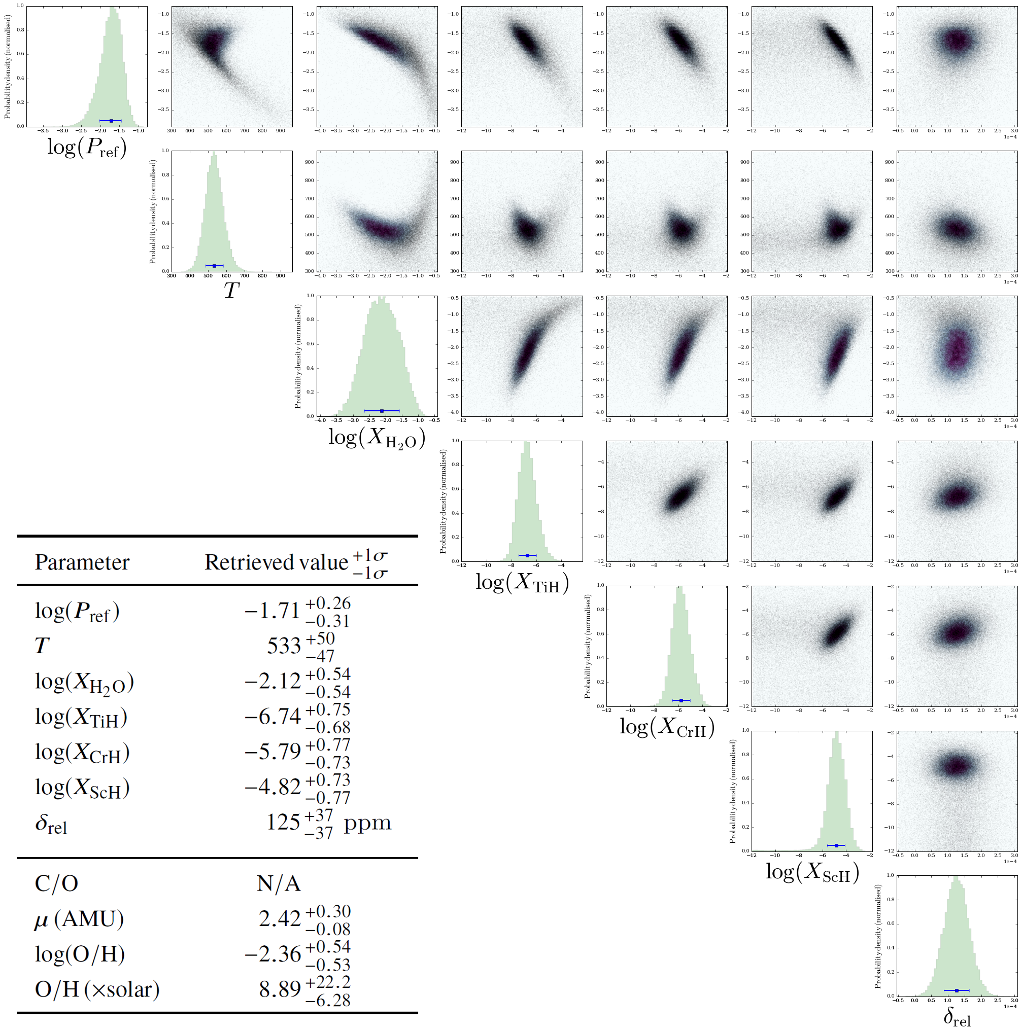 Figure 9
| P-T profile | ||
|---|---|---|
| Uniform | – | |
| Log-uniform | – | |
| Log-uniform | – | |
| Log-uniform | – | |
| Uniform | – | |
| Composition | ||
| Log-uniform | – | |
| Clouds | ||
| Log-uniform | – | |
| Uniform | – | |
| Log-uniform | – | |
| Uniform | ||
| Other | ||
| Uniform | – ppm |
| Evidence | ||||
| Best-fit | ||||
| Bayes | ||||
| Factor | ||||
| Significance | ||||
| of Ref. | ||||
| Full Chem | Ref. | Ref. | ||
| No H2+He | ||||
| No H2O | ||||
| No CH4 | N/A | |||
| No NH3 | N/A | |||
| No HCN | N/A | |||
| No CO | N/A | |||
| No CO2 | N/A | |||
| No C2H2 | N/A | |||
| No Na | N/A | |||
| No K | N/A | |||
| No Li | N/A | |||
| No TiO | N/A | |||
| No VO | N/A | |||
| No AlO | N/A | |||
| No CaO | N/A | |||
| No TiH | ||||
| No CrH | ||||
| No FeH | N/A | |||
| No ScH | ||||
| No ScH or AlO | ||||
| No M-Oxides | N/A | |||
| No M-Hydrides |
| Evidence | ||||
| Best-fit | ||||
| Bayes | ||||
| Factor | ||||
| Significance | ||||
| of Ref. | ||||
| P-T + Clouds | Ref. | Ref. | ||
| No Haze | N/A | |||
| Clear Skies | N/A | |||
| Iso + Clouds | Ref. | Ref. | ||
| No Haze | N/A | |||
| Clear Skies | N/A |
| Mode | GTO | |||
|---|---|---|---|---|
| NIRISS SOSS | hr | |||
| “ " | “ " | “ " | “ " | |
| NIRCam F322W2 | hr | |||
| NIRSpec G395H | hr | |||
| NIRCam F444W | hr | |||
| MIRI LRS | hr |
| Evidence | ||||
| Best-fit | ||||
| Bayes | ||||
| Factor | ||||
| Significance | ||||
| of Ref. | ||||
| Full Chem | Ref. | Ref. | ||
| No H2+He | ||||
| No H2O | ||||
| No CH4 | ||||
| No NH3 | N/A | |||
| No CO | ||||
| No CO2 | ||||
| No AlO | N/A | |||
| No TiH | ||||
| No CrH | ||||
| No ScH | ||||
| No M-Hydrides |
| Evidence | ||||
| Best-fit | ||||
| Bayes | ||||
| Factor | ||||
| Significance | ||||
| of Ref. | ||||
| Full Chem | Ref. | Ref. | ||
| No H2+He | ||||
| No H2O | ||||
| No Na | N/A | |||
| No K | N/A | |||
| No Li | N/A | |||
| No TiO | N/A | |||
| No VO | N/A | |||
| No AlO | N/A | |||
| No CaO | N/A | |||
| No TiH | N/A | |||
| No CrH | ||||
| No FeH | N/A | |||
| No ScH | ||||
| No M-Oxides | N/A | |||
| No M-Hydrides |
| Evidence | ||||
| Best-fit | ||||
| Bayes | ||||
| Factor | ||||
| Significance | ||||
| of Ref. | ||||
| P-T + Clouds | Ref. | Ref. | ||
| No Haze | N/A | |||
| Clear Skies | N/A | |||
| Iso + Clouds | Ref. | Ref. | ||
| No Haze | N/A | |||
| Clear Skies | N/A |
Peer Reviews
No public reviews on file for this paper yet. If you reviewed it on a platform where reviews are public (OpenReview, ICLR, NeurIPS, ICML), you can paste yours below so the community can read it here.
Videos
No videos yet. Explain this paper in a talk, walkthrough, or lecture? Add one.
The Metal-Rich Atmosphere of the Neptune HAT-P-26b
Ryan J. MacDonald1 & Nikku Madhusudhan1
1Institute of Astronomy, University of Cambridge, Madingley Road, Cambridge, CB3 0HA, UK Email: [email protected]: [email protected]
(Accepted 13 March 2019. Received 8 March 2019; in original form 23 January 2019)
Abstract
Transmission spectroscopy is enabling precise measurements of atmospheric H2O abundances for numerous giant exoplanets. For hot Jupiters, relating H2O abundances to metallicities provides a powerful probe of their formation conditions. However, metallicity measurements for Neptune-mass exoplanets are only now becoming viable. Exo-Neptunes are expected to possess super-solar metallicities from accretion of H2O-rich and solid-rich planetesimals. However, initial investigations into the exo-Neptune HAT-P-26b suggested a significantly lower metallicity than predicted by the core-accretion theory of planetary formation and solar system expectations from Uranus and Neptune. Here, we report an extensive atmospheric retrieval analysis of HAT-P-26b, combining all available observations, to reveal its composition, temperature structure, and cloud properties. Our analysis reveals an atmosphere containing H2O, an O/H of solar, and C/O (to 2). This updated metallicity, the most precise exo-Neptune metallicity reported to date, suggests a formation history with significant planetesimal accretion, albeit below that of Uranus and Neptune. We additionally report evidence for metal hydrides at 4.1 confidence. Potential candidates are identified as TiH (3.6), CrH (2.1), or ScH (1.8). Maintaining gas-phase metal hydrides at the derived temperature ( K) necessitates strong disequilibrium processes or external replenishment. Finally, we simulate the James Webb Space Telescope Guaranteed Time Observations for HAT-P-26b. Assuming a composition consistent with current observations, we predict JWST can detect H2O (at 29), CH4 (6.2), CO2 (13), and CO (3.7), thereby improving metallicity and C/O precision to 0.2 dex and 0.35 dex, respectively. Furthermore, NIRISS observations could detect several metal hydrides at 5 confidence.
keywords:
planets and satellites: atmospheres — planets and satellites: individual (HAT-P-26b) — methods: data analysis — techniques: spectroscopic
††pubyear: 2019††pagerange: The Metal-Rich Atmosphere of the Neptune HAT-P-26b–A
1 Introduction
Transmission spectroscopy has opened an unprecedented window into the atmospheric composition of exoplanets. Recent years have seen detections of multiple atomic and molecular species (e.g Snellen et al., 2010; Deming et al., 2013; Macintosh et al., 2015; Sedaghati et al., 2017; Hoeijmakers et al., 2018). Beyond detections, atmospheric retrieval techniques have enabled measurements of the abundances of chemical species (see Madhusudhan, 2018, for a recent review). By constraining the atmospheric composition, especially the H2O inventory, crucial clues are provided to identify formation scenarios (Öberg et al., 2011; Madhusudhan et al., 2014b; Mordasini et al., 2016). The most precise constraints have arisen from studies of hot Jupiters, as their extended atmospheres enhance the viability of transmission spectroscopy. Studies of hot Jupiters have reported H2O abundances implying a range of O/H ratios, from nearly solar () (Kreidberg et al., 2014; Line et al., 2016; Sing et al., 2016) to significantly sub-solar (Madhusudhan et al., 2014a; Barstow et al., 2016; Pinhas et al., 2019).
By contrast, the atmospheric composition of lower mass exoplanets, including exo-Neptunes and super-Earths, has proven challenging to constrain. In the solar system, lower mass planets possess atmospheres with an increasing fraction of heavy elements – termed the atmospheric metallicity. The metallicity of the solar system giants is commonly expressed in terms of the atmospheric C/H ratio, as derived from CH4 abundances. For Jupiter and Saturn, C/H is solar and solar, respectively (Atreya et al., 2016), whilst the ice-giants Uranus and Neptune are solar (Karkoschka & Tomasko, 2011; Sromovsky et al., 2011). This trend is consistent with the core-accretion theory of planet formation (Pollack et al., 1996). If low mass exo-Neptunes form in the same manner, they are anticipated to contain substantially H2O enriched atmospheres due to accretion of water-rich planetesimals (Fortney et al., 2013). Alternatively, in situ formation close to the parent star, resulting in minimal contamination by planetesimals, should lead to H2/He dominated atmospheres similar to the stellar photosphere (Rogers et al., 2011). H2O abundances thereby offer insights into the accretion history and physical properties of the original planetesimal building blocks. Measuring the composition of exo-Neptunes thus provides a powerful avenue to differentiate between planet formation mechanisms.
Until recently, constraints on exo-Neptune metallicities have proven relatively inconclusive. GJ 436b possesses a flat transmission spectrum, frustrating attempts to measure its composition and detect H2O. One scenario is GJ 436b’s atmosphere is dominated by high-altitude clouds (Knutson et al., 2014), with another possibility being a high metallicity due to accretion of rocky planetesimals, as suggested by its dayside emission spectrum (Madhusudhan & Seager, 2011; Moses et al., 2013; Morley et al., 2017). The first detection of H2O in an exo-Neptune was reported by Fraine et al. (2014) for HAT-P-11b’s atmosphere, though the derived metallicity (1-700 solar, to ) is consistent with both a nearly pure H2/He envelope and a wide range of core accretion scenarios.
Recently, the transmission spectrum of the exo-Neptune HAT-P-26b has provided a high-significance H2O detection (Wakeford et al., 2017). HAT-P-26b is a 4.23 day period exoplanet with and (Hartman et al., 2011; Wakeford et al., 2017), implying ms*-2*. The combination of low gravity and high temperature ( = 990 K) results in an extended atmosphere ideal for transmission spectroscopy. The first observations of HAT-P-26b’s transmission spectrum, using Magellan and Spitzer, were obtained by Stevenson et al. (2016). They reported evidence of H2O, though their data could not differentiate between a high metallicity ( solar) clear atmosphere and a solar metallicity atmosphere with a 10 mbar cloud deck. Wakeford et al. (2017) obtained additional visible and infrared transmission spectra with Hubble. This spectrum enabled them to report the first well-constrained metallicity in an exo-Neptune: O/H = solar (to ) – notably smaller than the solar that would be expected for a planet of this mass from core-accretion scenarios (Fortney et al., 2013).
However, no attempt has been made to simultaneously deduce the implications of these two datasets. In this work, we present a comprehensive atmospheric retrieval analysis, using all available observations, to derive the composition, metallicity, and other properties of HAT-P-26b’s atmosphere. As the lowest mass exoplanet with a detected spectral feature in primary transit, HAT-P-26b is presently our best window into formation mechanisms of Neptune-mass exoplanets. HAT-P-26b will also be observed during the James Webb Space Telescope’s (JWST) Guaranteed Time Observations (GTO), for which we offer predictions.
In what follows, the observations of HAT-P-26b are outlined in §2. We describe our atmospheric models and retrieval architecture in §3. The derived atmospheric properties of HAT-P-26b are presented in §4. Predictions for JWST’s GTO observations are offered in §5. Finally, in §6 we summarise our results and discuss the implications.
2 The Transmission Spectrum of HAT-P-26b
The transmission spectrum of HAT-P-26b comprises 50 observations from both ground and space-based facilities. Magellan Low Dispersion Survey Spectrograph 3 (LDSS-3C) observations (Stevenson et al., 2016) are complimented by Hubble Space Telescope Imaging Spectrograph (STIS) and Wide Field Camera 3 (WFC3) grism observations, along with Spitzer Infrared Array Camera (IRAC) photometric observations (Wakeford et al., 2017). The observed transit depths in each instrument mode are shown in Figure 1.
The combined set of observations offers continuous wavelength coverage across the visible and near-infrared, from . The Spitzer IRAC channels additionally cover the regions surrounding 3.6 & 4.5 . The STIS G750L observations span the range 0.5-1.0 , with a mean spectral resolution and mean precision ppm. The LDSS-3C red observations span the range 0.7-1.0 , with mean 70 and mean precision 155 ppm. The WFC3 G102 and G141 grism observations span the ranges 0.8-1.1 and 1.1-1.6 , respectively, with corresponding resolutions 40 and 60, and mean precisions of 70 and 50 ppm. The precision of the two Spitzer IRAC photometric observations are 130 and 170 ppm.
Our analysis considers these observations as a given input. The data reduction of the transit observations is discussed in detail in Stevenson et al. (2016); Wakeford et al. (2016); Sing et al. (2016); Wakeford et al. (2017). We note that Spitzer observations are available from both Stevenson et al. (2016) and Wakeford et al. (2017). Here we employ only those from Wakeford et al. (2017), to ensure consistent data reduction across the space-based observations. To account for the possibility of differing normalisations between the ground-based and space-based observations due to stellar variability or differing reduction procedures, we allow for a relative offset between these two datasets during our analysis. With the observations described, we proceed to detail our framework for inverting these observations to obtain the atmospheric state of HAT-P-26b.
3 Atmospheric Retrieval Architecture
We infer the atmospheric properties at HAT-P-26b’s day-night terminator using the radiative transfer and retrieval code POSEIDON (MacDonald & Madhusudhan, 2017a). This code couples a transmission spectrum forward model with a Bayesian parameter estimation and model comparison algorithm, enabling derivation of statistically rigorous atmospheric parameter constraints and detection significances for various atmospheric model components. POSEIDON has previously been applied to the atmospheric retrieval of hot Jupiters (MacDonald & Madhusudhan, 2017a, b; Sedaghati et al., 2017; Kilpatrick et al., 2018). Here, we outline salient aspects as they apply to the present analysis - in particular, recent updates to generalise its scope to exo-Neptune atmospheres.
We describe our atmospheric models in section 3.1, generation of transmission spectra in section 3.2, and the parameters specifying each model atmosphere in section 3.3.
3.1 Atmospheric models
We model the terminator region of HAT-P-26b’s atmosphere in a plane-parallel geometry. The atmosphere is discretised into 100 axially-symmetric layers about the observer’s line-of-sight, uniformly spaced in log-pressure from to bar. The temperature in each layer, expressed as a function of pressure, determines the number density in each layer via the ideal gas law. The atmospheric composition, described in section 3.1.1, specifies the atmospheric mean molecular weight. The planetary radius and surface gravity are placed at a parameterised reference pressure, where they iteratively specify a radial distance grid under the assumption of hydrostatic equilibrium. Clouds and hazes, along with partial cloud coverage, are included as potential components of the atmosphere, as discussed in section 3.1.2.
3.1.1 Molecular & atomic opacities
A wide range of potential chemical species and compositions need to be considered when modelling the atmospheres of exo-Neptunes (Madhusudhan et al., 2016). On the one-hand, atmospheres could be H2-He dominated with other chemical species, such as H2O and CO, present as trace gases – as for hot Jupiters with near-solar or sub-solar metallicity. Alternatively, a wide range of high mean molecular weight atmospheres, especially H2O or CO2 rich compositions, are also a possibility at higher metallicities (Moses et al., 2013).
We consider many prospective sources of infrared and visible opacity. Standard carbon, oxygen, and nitrogen-bearing species with well-known infrared absorption features are included: H2O, CH4, NH3, HCN, CO, CO2, and C2H2. H2 and He are treated as a single gaseous species, with a fixed solar H2/He ratio of 0.17 assumed. Given the suggestions of substructure in HAT-P-26b’s visible-wavelength transmission spectrum (Figure 1), we also consider chemical species with prominent optical cross sections. We therefore include alkali metals along with metal oxides and hydrides (Sharp & Burrows, 2007). Specifically, we consider: Na, K, Li, TiO, VO, AlO, CaO, TiH, CrH, FeH, and ScH. Absorption cross sections for these species are shown in Figure 2. The criterion for including an optical absorber in our models was taken to be cm2 at the equilibrium temperature of HAT-P-26b – where ‘vis’ indicates wavelengths covering the visible portion of the observations (). This somewhat arbitrary criterion renders the dimensionality of the parameter space tractable for exploration by removing species with negligible absorption cross sections (see Tennyson & Yurchenko, 2018, for a visual demonstration). We have verified that including additional species with weaker cross sections do not modify our results.
The molecular and atomic cross section database employed by POSEIDON has recently undergone a substantial upgrade. Compared to the cross sections used in MacDonald & Madhusudhan (2017a), the spectral resolution has been increased by a factor of 100 (to = 0.01 cm*-1*), the temperature and pressure coverage has been extended ( bar and K, respectively), and pressure broadening now accounts for H2 and He (in an 85 to 15 mixture) instead of air broadening. The line list sources have also been revised to reflect the current state of the art. We no longer use line lists from the HITEMP-2010 database, opting instead for the more recent POKAZATEL H2O line list (Polyansky et al., 2018), the Li et al. (2015) CO line list, and CDSD-4000 for CO2 (Tashkun & Perevalov, 2011). We have also upgraded CH4 to the latest 34to10 EXOMOL line list (Yurchenko et al., 2017), C2H2 to ASD-1000 (Lyulin & Perevalov, 2017), and the atomic transitions to VALD3 (Pakhomov et al., 2017). Line lists for the remaining molecules are taken from ExoMol (Tennyson et al., 2016), in particular Burrows et al. (2005, 2002) for TiH and CrH and Lodi et al. (2015) for ScH. The calculation of these cross sections follows a similar method to Hedges & Madhusudhan (2016) and Gandhi & Madhusudhan (2017).
We also include collisionally-induced absorption (CIA) and Rayleigh scattering. CIA due to H2-H2, H2-He, and H2-CH4 is taken from HITRAN (Richard et al., 2012), whilst Rayleigh scattering cross section for H2, He, and H2O are derived from refractive indices in various sources (Hohm, 1993; Mansfield & Peck, 1969; Hill & Lawrence, 1986).
3.1.2 Treatment of clouds and hazes
An important source of opacity can be provided by clouds and hazes. Here, we consider clouds to constitute an opaque deck located at , below which no electromagnetic radiation may pass. This effectively corresponds to the grey, large particle size limit of Mie scattering (e.g Kitzmann & Heng, 2018). Hazes, however, are distributed uniformly throughout the atmosphere with an extinction coefficient given by a two-parameter power law (Lecavelier des Etangs et al., 2008): , where is a reference wavelength (350 nm), is the -Rayleigh scattering cross section at the reference wavelength (), is the ‘Rayleigh enhancement factor’, and is the ‘scattering slope’. This ‘enhanced-Rayleigh’ slope accounts for the effect of small particle sizes, with the parameter in principle indicative of the aerosol causing the slope (Pinhas & Madhusudhan, 2017). We additionally allow for inhomogeneous terminator cloud and haze distributions (Line & Parmentier, 2016; MacDonald & Madhusudhan, 2017a), with a terminator coverage fraction . The effect of this ‘patchy cloud’ on the radiative transfer calculation is espoused in the next section.
3.2 Radiative transfer
Transmission spectra are computed by solving the equation of radiative transfer under a plane-parallel geometry. Here we outline the essential aspects, with a comprehensive discussion given in MacDonald & Madhusudhan (2017a). The slant optical depth for a given impact parameter is obtained by integrating the atmospheric extinction coefficient – including chemical and cloud / haze opacity – along the observer’s line of sight. The effective planetary radius of an axially-symmetric atmosphere, at a given wavelength, is computed by integrating the atmospheric transmission, , over successive annuli:
[TABLE]
where is the radial extent of the modelled atmosphere, is the slant optical depth at wavelength , and is the impact parameter of a given ray. A ‘one-dimensional’ transmission spectrum can then be computed: , where is the stellar radius ( for HAT-P-26).
Azimuthal inhomogeneities are included via a linear superposition of transit depths, weighted by the coverage fraction of a given region. Here, we consider the possibility of inhomogeneous clouds (Line & Parmentier, 2016) and hazes by superimposing cloudy and cloud-free models:
[TABLE]
where is the terminator cloud coverage fraction. This two-dimensional cloud / haze prescription facilitates the breaking of many cloud-haze-composition degeneracies that can manifest in strictly one-dimensional cloud models (Benneke & Seager, 2013; MacDonald & Madhusudhan, 2017a).
We evaluate transmission spectra at a constant spectral resolution of from 0.4-5.2 m. Model spectra are convolved with the relevant grism point spread functions and integrated over instrument response curves to produce binned model points at the resolution of the observations. Spitzer model points are produced by integrating over the IRAC 3.6 m and 4.5 m photometric instrument functions.
3.3 Atmospheric parameterisation
Each model atmosphere is expressed in terms of a parametric state vector, which encodes the pressure-temperature profile, atmospheric composition, and cloud / haze properties. The pressure-temperature (P-T) profile comprises either the flexible 6 parameter shape from Madhusudhan & Seager (2009) (re-expressed in terms of the 1mbar temperature) or an isotherm, supplemented by – the a priori unknown pressure at . The atmospheric composition (section 3.1.1) is encoded via up to 18 volume mixing ratios, , assumed to be uniform both in altitude and across the terminator. Clouds and hazes are described by the 4 parameter prescription of MacDonald & Madhusudhan (2017a) (section 3.1.2). A relative offset between the Stevenson et al. (2016) and Wakeford et al. (2017) observations, , is prescribed, as discussed in section 2. Our models thus have a maximum of 30 free parameters, summarised in Table 1.
Priors for each parameter are taken as either uniform or uniform-in-the-logarithm, depending on whether the range is less than or more than two orders of magnitude, respectively. The P-T profile and cloud parameter priors are chosen to be generous and uninformative, for the reasoning discussed in MacDonald & Madhusudhan (2017a). Mixing ratios have an upper limit of ( 50%), with the remainder assumed to comprise H2 and He in solar proportions. Strictly speaking, truly permutation invariant mixing ratios (e.g. equal a priori probabilities for a CO2 or H2O dominated atmosphere vs. a H2-He dominated atmosphere) requires usage of a flat Dirchlet prior (uniform over the unit simplex) (Benneke & Seager, 2012). This approach is, however, computationally expensive for mixing ratios, so we implicitly assume that the atmosphere of HAT-P-26b does not have via our usage of bounded log-uniform priors on the other species. We have verified that usage of a Dirchlet prior results in no notable differences in the retrieved parameters for this planet.
3.4 Retrieval methodology
POSEIDON is capable of both Bayesian parameter estimation and model comparison. For reporting parameter constraints, we utilise the complete model including all 30 parameters described in section 3.3 – this ensures any degeneracies, such as between clouds and composition, are captured via posterior marginalisation. As a guiding principle, we also employ nested Bayesian model comparison using the computed Bayesian evidences of competing models to identify the simplest model compatible with the observations (see MacDonald & Madhusudhan, 2017a, for a full description of statistical aspects of our retrieval methodology). This enables direct assessment of model complexity via evaluating the statistical significance of each model component (e.g. detection significances of chemical species, clouds, etc).
We conducted over 50 atmospheric retrievals in the course of our investigation. Each multi-dimensional parameter space is explored via the multimodal nested sampling algorithm MultiNest (Feroz & Hobson, 2008; Feroz et al., 2009), as implemented by the python wrapper PyMultiNest (Buchner et al., 2014). Our retrievals typically employ 4000 MultiNest live points, with a Bayesian evidence termination error of . A typical 30 dimensional retrieval then results in the computation of transmission spectra. Using this methodology, we now proceed to describe constraints on the atmospheric properties of HAT-P-26b, including its metallicity, before assessing the degree of model complexity current observations warrant.
4 The Atmosphere of HAT-P-26b
We here present our inferences into the atmospheric properties of HAT-P-26b. We begin in section 4.1 with a brief discussion on the overall quality of our spectral fits to the observations. We then examine the atmospheric composition of HAT-P-26b in section 4.2, constraints on clouds and the pressure-temperature (P-T) profile in sections 4.3 and 4.4, respectively, before examining the minimal model complexity necessary to adequately fit the observations in section 4.5. We detail in appendix A an equivalent retrieval analysis utilising only observations from Wakeford et al. (2017).
4.1 Retrieved transmission spectrum
Figure 3 shows the retrieved transmission spectrum of HAT-P-26b. This corresponds to the ‘full’ 30-dimensional model described in section 3.3, including a wide range of chemical species, non-isothermal P-T profiles, clouds and hazes, and a relative offset between the Stevenson et al. (2016) and Wakeford et al. (2017) datasets. The posterior distribution from this retrieval is available as supplementary online material. Our best-fitting model spectrum, binned to the resolution of the observations, lies within 1 for 66% of the observations (33 out of 50, yielding ). Much of the spectral structure in the infrared is explained by H2O, as concluded by Wakeford et al. (2017). The attribution of spectral features at visible wavelengths, well-fit by our models, to specific species is detailed in section 4.2.1.
Before deriving atmospheric properties, we first assessed if a relative offset, , was necessary. We ran an identical retrieval with the raw data alone, and conducted a Bayesian model comparison between this model and the full model. The result was a Bayes factor of 7.86 in favour of the full model (equivalent to 2.6), hence we include as a parameter in all subsequent retrievals. The likely reason for the retrieved offset, ppm, is the likelihood penalty induced by the cluster of LDSS-3C observations around 0.72 (and to a lesser extent around 0.99 ) that are much lower than the other data points and are difficult to explain with our models. For example, the data around 0.72 , are far lower than would be expected of pure H2 Rayleigh scattering without any additional sources of opacity. Stevenson et al. (2016) has previously identified these points as outliers, which can potentially be attributed to fringing (Wakeford et al., 2017). Nevertheless, the retrieved parameters are consistent even when not using a relative offset. We turn now to atmospheric inferences from our spectral retrievals.
4.2 Composition
We first describe the atmospheric composition of HAT-P-26b obtained from our retrieval analysis. We establish in section 4.2.1 which chemical species included in our models are indicated by the observations, along with their associated statistical significances. We examine spectral features of each indicated species in section 4.2.2. Constraints on the abundances of these species are reported in section 4.2.3. Finally, in section 4.2.4, constraints on derived atmospheric properties, such as the metallicity and C/O are presented.
4.2.1 Detections
We establish at high significance that the atmosphere of HAT-P-26b is primarily H2+He dominated, with H2O as a secondary component. We detect H2O at confidence via a nested Bayesian model comparison (see below), in agreement with the previous detection of H2O by Wakeford et al. (2017). Notably, H2O is the only considered species that explains the broad and absorption features (see Figure 3). Following the confirmation of H2O, we directly computed the significance of H2+He as the background gas by considering a model with no H2+He, H2O as the dominant gas, and all other species as trace gases. This model poorly fit the observations – primarily due to the resulting high mean molecular weight of atomic mass units – enabling us to establish at confidence that H2+He must be the dominant background gas.
The reference list from the paper itself. Each links out to its DOI / PubMed record.
- 1Ackerman & Marley (2001) Ackerman A. S., Marley M. S., 2001, Ap J , 556, 872 · doi ↗
- 2Asplund et al. (2009) Asplund M., Grevesse N., Sauval A. J., Scott P., 2009, Annu. Rev. Astron. Astrophys , 47, 481 · doi ↗
- 3Atreya et al. (2016) Atreya S. K., Crida A., Guillot T., Lunine J. I., Madhusudhan N., Mousis O., 2016, preprint, ( ar Xiv:1606.04510 )
- 4Barstow et al. (2013) Barstow J. K., Aigrain S., Irwin P. G. J., Bowles N., Fletcher L. N., Lee J.-M., 2013, MNRAS , 430, 1188 · doi ↗
- 5Barstow et al. (2015) Barstow J. K., Aigrain S., Irwin P. G. J., Kendrew S., Fletcher L. N., 2015, MNRAS , 448, 2546 · doi ↗
- 6Barstow et al. (2016) Barstow J. K., Aigrain S., Irwin P. G. J., Sing D. K., 2016, Astrophys. J. , 834, 50 · doi ↗
- 7Batalha & Line (2017) Batalha N. E., Line M. R., 2017, AJ , 153, 151 · doi ↗
- 8Batalha et al. (2017) Batalha N. E., et al., 2017, PASP , 129, 064501 · doi ↗