Brushing up a theorem by Lehel Banjai on the convergence of Trapezoidal Rule Convolution Quadrature
Hasan Eruslu, Francisco-Javier Sayas

TL;DR
This paper clarifies the convergence properties of the Trapezoidal Rule Convolution Quadrature method for hyperbolic problems, building on Banjai's and Lubich's foundational work to improve understanding of its time-dependent estimates.
Contribution
It provides detailed explanations and clarifications of the convergence estimates for the Trapezoidal Rule Convolution Quadrature, enhancing comprehension of its dependence on the time variable.
Findings
Refined convergence estimates for the method
Clarified dependence on time variable
Improved understanding of hyperbolic problem applications
Abstract
This document is made up of two different units. One of them is a regular terse research article, whereas the other one is the detailed and independently written explanations for the paper, so that readers of the short paper do not need to go over all the cumbersome computations. The goal is to clarify the dependence with respect to the time variable of some estimates about the convergence of the Trapezoidal Rule based Convolution Quadrature method applied to hyperbolic problems. This requires a careful investigation of the article of Lehel Banjai where the first convergence estimates were introduced, and of some technical results from a classical paper of Christian Lubich.
Click any figure to enlarge with its caption.
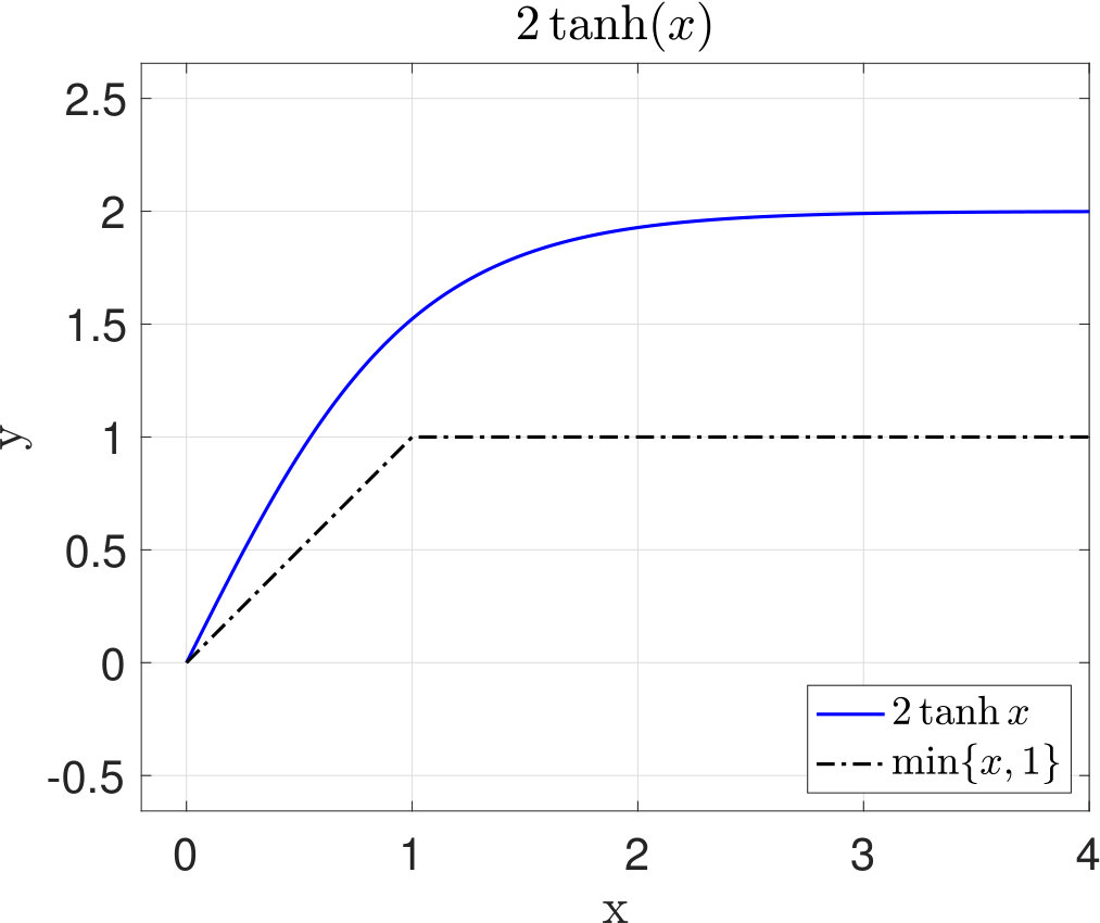 Figure 1
Peer Reviews
No public reviews on file for this paper yet. If you reviewed it on a platform where reviews are public (OpenReview, ICLR, NeurIPS, ICML), you can paste yours below so the community can read it here.
Code & Models
Videos
No videos yet. Explain this paper in a talk, walkthrough, or lecture? Add one.
Taxonomy
TopicsFractional Differential Equations Solutions · Iterative Methods for Nonlinear Equations · Numerical methods for differential equations
Brushing up a theorem by Lehel Banjai
on the convergence of
Trapezoidal Rule Convolution Quadrature111Both authors are partially supported by NSF grant DMS 1818867
Hasan Eruslu222Department of Mathematical Sciences, University of Delaware. [email protected], Francisco-Javier Sayas333Department of Mathematical Sciences, University of Delaware. [email protected]
University of Delaware
Abstract
This document is made up of two different units. One of them is a regular terse research article, whereas the other one is the detailed and independently written explanations for the paper, so that readers of the short paper do not need to go over all the cumbersome computations. The goal is to clarify the dependence with respect to the time variable of some estimates about the convergence of the Trapezoidal Rule based Convolution Quadrature method applied to hyperbolic problems. This requires a careful investigation of the article of Lehel Banjai where the first convergence estimates were introduced, and of some technical results from a classical paper of Christian Lubich.
Key words. Convolution quadrature, Laplace transforms, Trapezoidal rule
AMS Classification. 26D10, 30A10, 44A10, 65L06
The actual article
1 Introduction
Without much practical motivation, let us explain what the goals of this article are. We first need to give a short introduction to the Convolution Quadrature (CQ) techniques to approximate causal distributional convolutions by the systematic use of the symbol (Laplace transform) of the operator. We will be interested in particular in the Trapezoidal Rule (TR) based CQ method. The reason for this is multiple. The original work of Lubich [12] extends his results [11] on multistep CQ for parabolic problems (parabolic character is reflected in having the Laplace transform of the operator extended to a sector around the negative axis) to hyperbolic problems (where the Laplace transform is defined only on a half plane). Because of Dahlquist barrier, only second order multistep CQ methods are available for hyperbolic problems, and the analysis in [12] excludes the TRCQ method for technical reasons. However, it is well known (and it has been tested repeatedly in the world of Time Domain Boundary Integral Equations – TDBIE) that the TR based method outperforms the first order backward Euler method and BDF2 which is much too dispersive. Note that Runge-Kutta CQ schemes [13] with higher order and less dispersion are also available, and that a detailed time domain analysis is also missing from [4] and [5].
As a warning to the reader, let us say that this paper is quite technical, but it closes an important question (left open in the monograph [14]) as how error estimates for TRCQ behave polynomially in time and there is no hidden Gronwall Lemma argument that would lead to exponential in time upper bounds. In the appendix of Banjai’s paper [3], which we are polishing up, the estimates are written for finite time intervals and the behavior with respect to the final time is not specified.
Let us now give a crash course on the mathematical aspects of TRCQ. For algorithmic and practical introductions to the CQ methods, we recommend [7] and [9]. For a detailed introduction to the distributional language required for a deep understanding of CQ applied to TDBIE, see [14]. Our starting point is a couple of Banach spaces and and the space of bounded linear operators , whose norm will be denoted . The second ingredient is the symbol of a momentarily hidden convolutional operator: we assume that we have an analytic function
[TABLE]
satisfying
[TABLE]
where is non-increasing and for some when is close to zero. We will be interested in symbols where the parameter in (1.2), but we will show some results (based on [12]), where we will use negative values of as well. The TRCQ approximation of this symbol consists of defining
[TABLE]
Here is the constant time-step (see more explanations later) of the underlying TR scheme (recall that in (1.3) is the characteristic function of the TR scheme). We will show that for every , so that the definition of makes sense, and we will also show that is a symbol with properties (1.1)-(1.2), although with different parameters to those of .
Properties (1.1)-(1.2) ensure that is the Laplace transform of a causal tempered -valued distribution, which we will name . Moreover, is the Laplace transform of the distributional time derivative of a certain order (depending on ) applied to a function which is causal ( in ), continuous, and polynomialy bounded. See full details in [14, Chapters 2 & 3]. Under these conditions, we can define a convolutional product of the operator valued acting on a causal -valued distribution , outputting a causal -valued distribution. Informally, we are dealing with
[TABLE]
Similary, is the Laplace transform of a causal tempered -valued distribution , and the TRCQ approximation consists of substituting by . In practice, what is computed are the values
[TABLE]
although the theory is developed for the full real distribution . The time-step values of are given by the discrete convolution
[TABLE]
In practice, the discrete convolutions (1.5) are computed using a parallel process, FFTs, and some kind of contour integration [6, 7, 9]. If applied to a linear system of ODEs with vanishing initial conditions, TRCQ is reduced to the TR scheme applied to the original system. One of the main field of applications of CQ for hyperbolic problems is in the area of TDBIE, using the language and ideas of the seminal papers of Bamberger and Ha-Duong [1, 2]. More examples, including coupled systems of wave equations in bounded domains with TDBIE in their exterior, can be found in [10]. More recently, a rich domain of applications of CQ has been opened in the numerical approximation of propagation of viscoelastic waves [8].
2 The main theorem
To state the main theorem, we will use the Sobolev-Bochner space
[TABLE]
Note that if , then for We will also need the -th order linear differential operator
[TABLE]
The remainder of this paper will consist of a proof of the next theorem. Some easy (but somewhat cumbersome details) are avoided. The reader is welcome to look for the arXiv version of this document to find a fastidiously detailed proof of each single step.
Theorem 2.1**.**
Let satisfy (1.1)-(1.2) for and with fulfilling the conditions given after (1.2). Let be the distributional inverse Laplace transform of and be its TRCQ approximation, i.e., the inverse Laplace transform of given in (1.3), for any given time-step . Consider the parameters
[TABLE]
For any and ,we have
[TABLE]
where
[TABLE]
Note that
[TABLE]
3 The TRCQ discrete derivative
We now introduce some key functions for the estimates that follow. First of all, note that the function
[TABLE]
is even and analytic in . We then define
[TABLE]
and note that is also analytic in the same disk and that the function is strictly increasing, non-negative and diverges as . Therefore, there exists a unique
[TABLE]
Next, we define
[TABLE]
and notice that . Using these, we are going to present some properties of the characteristic function of the TR rule. At the end of this section we will give a technical result which will be a key tool in the proof of Theorem 2.1.
Lemma 3.1**.**
The following inequalities hold:
- (a)
* for all .* 2. (b)
* for all .* 3. (c)
* for all and all with .* 4. (d)
* for all with .*
Proof.
For , it is easy to verify that Using this with for and noting that , we write
[TABLE]
The proof of (a) follows then from
[TABLE]
We prove (b) by using (3.1) together with the triangle and reverse triangle inequalities in the following way
[TABLE]
To show (c) and (d), we define
[TABLE]
and observe that which holds because of the definition of . Using this, it is not hard to see that
[TABLE]
which proves (c). For (d), we write
[TABLE]
Note that the result is stated (and later used) only for , which ensures that the right-hand side of the above inequality is positive. ∎
The discrete version of this lemma will be a building block for the rest of this paper.
Proposition 3.2**.**
For , the following inequalities hold:
- (a)
* for all .* 2. (b)
* for all .* 3. (c)
* for all and all with .* 4. (d)
* for all with .*
Proof.
The result follows from Lemma 3.1 by simply inserting and noting that . ∎
Lemma 3.3**.**
For and we have
[TABLE]
Proof.
We can easily estimate
[TABLE]
This finishes the proof. ∎
Proposition 3.4**.**
If with , and
[TABLE]
then for all we have
[TABLE]
where is a positive constant depending only on .
Proof.
For the sake of convenience, we will abuse notation by eliminating the explicit dependence with respect to in
[TABLE]
where is fixed. We now take an arbitrary but fixed value of , and define the integration regions and , covering the entire real line. We split our target integral into three pieces, and work on them one by one
[TABLE]
Since on and is increasing, Proposition 3.2(c) yields
[TABLE]
For the second integral, using Proposition 3.2(b) and the fact that on , we have
[TABLE]
Lastly, the definition of implies that
[TABLE]
Combining these three estimates we can write
[TABLE]
where
[TABLE]
The definition of implies that
[TABLE]
Therefore, using that for and Lemma 3.3, we can write
[TABLE]
This inequality and (3.2) prove the result with . However, the dependence on is limited to , so we can eliminate by taking in the bounds. ∎
4 Revisiting a result of Christian Lubich
In this section, we work on some key results when satisfies (1.1)-(1.2) with . We start with showing that , like , is the Laplace transform of a causal tempered -valued distribution. In Proposition 4.4 we revisit Lubich’s [12, Theorem 3.1], and prove it for by including the case which was missing in that manuscript, and add the explicit dependence with respect to the time variable in the bounds.
Proposition 4.1**.**
If satisfies (1.1)-(1.2) with , then
- (a)
* for all .* 2. (b)
* for all .* 3. (c)
* for all .*
In the above bounds
[TABLE]
The functions and are defined on and they can be bounded by a negative power of as . The function is defined on , is increasing, and when it diverges as .
Proof.
To prove (a), we first observe that Proposition 3.2(a) implies , therefore (1.2) gives
[TABLE]
The rest of the proof follows from Proposition 3.2(a) and the fact that and are non-decreasing functions on .
For (b), we use same ideas given in the proof of [14, Proposition 4.5.3]. Defining the curve with positive orientation, we write
[TABLE]
We finish the proof of (b) using the fact that and for .
To show (c), we write the following by using the Mean Value Theorem
[TABLE]
for some . Now, we define , and use (a) to write
[TABLE]
This can be bounded by observing
[TABLE]
and then using Proposition 3.2(a) and (d). We finish the proof by using Proposition 3.2(c) with and noting that .
∎
Lemma 4.2**.**
The following holds for all , , and :
- (a)
** 2. (b)
**
Proof.
In order to prove (a), for fixed and , we define the domains of integration and , which give
[TABLE]
We bound the first integral using the fact that on . We rewrite the second integral using a change of variables and bound it in the following way
[TABLE]
which finishes the proof of (a). We prove (b) by simply writing
[TABLE]
∎
Proposition 4.3**.**
If satisfies (1.1)-(1.2) with and , then for all we have
[TABLE]
where
[TABLE]
and is a positive constant depending only on .
Proof.
For fixed and we will make use of the following domains of integration
[TABLE]
and the notation . Using these we can write
[TABLE]
We bound the first integral on the right-hand side using Proposition 4.1(c) and Lemma 4.2(b)
[TABLE]
where is a positive constant depending only on . Next, with the help of Proposition 4.1(a) and Lemma 4.2(a), the second integral is bounded in the following way
[TABLE]
Here is a positive constant depending only on . Combining these estimates we write
[TABLE]
with . Note that this estimate holds for all , therefore we finish the proof by replacing the constant with . ∎
Proposition 4.4**.**
If satisfies (1.1)-(1.2) with , and with , then
[TABLE]
holds for all , where is a positive constant depending only on .
Proof.
For any and , using the inverse Laplace transformation, we write
[TABLE]
Next, the definition of Laplace transformation together with Proposition 4.3 and setting give
[TABLE]
Now, we are going to obtain an integral bound over the interval . For a fixed , we define the following function
[TABLE]
It is not hard to see that , in other words, satisfies the conditions of the proposition. Using the fact that on and on , we write
[TABLE]
which finishes the proof. ∎
5 Proof of Theorem 2.1
In this section we prove the main theorem. We start with presenting a lemma to obtain upper-bounds integrated over the interval rather than in the proof of the main theorem.
Lemma 5.1**.**
Let , , , and be a fixed real number. We define the function
[TABLE]
and, for , the integration operator
[TABLE]
The function
[TABLE]
satisfies that and on .
Proof.
We observe that, for , the functions
[TABLE]
vanish when . From there, it is not hard to see that . Next, since , we know that
[TABLE]
is also in , and so is . This shows that . The function and therefore . The rest of the proof follows from the fact that
[TABLE]
∎
Proposition 5.2**.**
Let with , and satisfy (1.1)-(1.2). We define such that
[TABLE]
The following estimate holds for all
[TABLE]
where
[TABLE]
and is a positive constant depending only on .
Proof.
For any , using the inverse Laplace transformation, we write
[TABLE]
where . Here, with the help of Proposition 3.4 and inserting , we obtain
[TABLE]
Now, our goal is to have an integral bound over the interval . To do that, for fixed , we consider the function introduced in Lemma 5.1. Since , in other words, it satisfies the conditions of this proposition, we can have the estimate (5.1) for as well. Therefore, using the properties of this function, we write
[TABLE]
This finishes the proof. ∎
Proof.
[Theorem 2.1] For , we define
[TABLE]
and
[TABLE]
Using these definitions it is not hard to see that
[TABLE]
Now, we will obtain bounds for the terms on the right-hand side. For the first term, since and
[TABLE]
where , we can use Proposition 4.4 to write
[TABLE]
Next, we bound the second term using Proposition 5.2 in the following way
[TABLE]
Here, using the definition of and Proposition 4.1(a) we have
[TABLE]
for all . Combining this with (5.2) finishes the proof. ∎
1 General concepts and definitions
We start with defining the set
[TABLE]
Following the notation of [14], we assume is analytic and satisfies
[TABLE]
where
- •
,
- •
is non-increasing on ,
- •
is polynomially bounded at .
The transfer function for the Trapezoidal rule is
[TABLE]
Equivalently, we can also write
[TABLE]
We will use the following notation in our temporal approximations
[TABLE]
and assume that temporal discretization parameter is bounded
[TABLE]
2 Technical results
Lemma 2.1**.**
The following properties hold for all :
- (a)
. 2. (b)
. 3. (c)
. 4. (d)
.
Proof.
To prove (a), we first observe that is increasing (see Figure 1) and
[TABLE]
therefore
[TABLE]
For the case , we define the function
[TABLE]
Since
[TABLE]
we know is concave. Using (2.1), we have
[TABLE]
and, therefore,
[TABLE]
which finishes (a). Part (b) follows from (a). For (c), using (a), we write
[TABLE]
This also implies (d). ∎
Proposition 2.2**.**
The following holds:
- (a)
* for all .* 2. (b)
* for all .* 3. (c)
* for all with .* 4. (d)
* for all and all with .* 5. (e)
* for all with .*
Here is such that , and
[TABLE]
where is analytic in with for all . The functions
[TABLE]
are increasing and they diverge as . Also note that .
Proof.
To prove (a), we first observe that the following holds for all
[TABLE]
Now, when we have . Therefore we can use (2.3) with , which gives
[TABLE]
The rest of the proof of (a) follows from Lemma 2.1(c).
To prove (b), using the triangle and reverse triangle inequalities, we write
[TABLE]
and therefore
[TABLE]
We then apply Lemma 2.1(d) to finish the proof.
To show (c), we write the following (see (1.2))
[TABLE]
and define . We know is an analytic odd function in , and , hence
[TABLE]
is an analytic even function in the same domain. As a consequence, we know that
[TABLE]
is analytic in . Using this, we can now write
[TABLE]
To finish this part of the proof, we define , which gives
[TABLE]
For (d), we first write
[TABLE]
where, because of (c), we know that
[TABLE]
Next, we compute
[TABLE]
and, using (2.7), we obtain
[TABLE]
which holds for all . Finally, using the fact that
[TABLE]
and the definition of the function , we write
[TABLE]
To prove (e), using (1.2) and (2.4), we write
[TABLE]
Therefore, for all , we have
[TABLE]
where we used (2.5) and (2.6) for the last inequality. Although (2.8) holds for all , it is not useful to have a negative lower bound. To avoid that, we investigate the function
[TABLE]
This function is increasing, since is increasing (see its definition (2.2)), it vanishes at , and diverges as . Hence, there is a unique such that
[TABLE]
and we will consider the inequality (2.8) when . ∎
Following result is the discrete counterpart of Proposition 2.2.
Proposition 2.3**.**
For as in (1.3), we have
- (a)
* for all .* 2. (b)
* for all .* 3. (c)
* for all and all with .* 4. (d)
* for all with .*
Proof.
Part (a) follows from Proposition 2.2(a) and the fact that
[TABLE]
Similarly, for (b), we use Proposition 2.2(b) to write
[TABLE]
To prove (c), we use Proposition 2.2(d) to show
[TABLE]
Finally, to prove (d), with the help of Proposition 2.2(e) we write
[TABLE]
which finishes the proof. ∎
3 Discrete differentiation
We will call a function causal, if for all . Next, we define the following Sobolev spaces for and Hilbert space
[TABLE]
Note that, for , we have
[TABLE]
and we know that the space
[TABLE]
is dense in . We will also make use of the following definition
[TABLE]
Before moving to the main result of this section, we are going to present some technical tools. The following lemma establishes a way of going from an integral in the Laplace domain to an integral in the time domain with a cost of two derivatives.
Lemma 3.1**.**
For and we have
[TABLE]
Proof.
We start with writing
[TABLE]
We can evaluate the integral on the right-hand side exactly
[TABLE]
For the other part, using the definition of the Laplace transform we write
[TABLE]
This finishes the proof. ∎
Lemma 3.2**.**
For all and we have
[TABLE]
Proof.
Using the Cauchy-Schwarz inequality and the fact that , we write
[TABLE]
which proves (3.1) for . When , we do the following
[TABLE]
where for the last inequality we use the case . ∎
Next result is a key ingredient in the proof of Theorem 5.2. We introduce the following notation
[TABLE]
Proposition 3.3**.**
Let , , and
[TABLE]
For all , we have
[TABLE]
where
[TABLE]
Proof.
We start with fixing . For an arbitrary and fixed , we define regions of the integration
[TABLE]
We also introduce the following notation for convenience
[TABLE]
Next, we split our target integral into three pieces
[TABLE]
Now we are going to work on integrals separately and establish some bounds in the Laplace domain.
When , we have . Therefore, using Proposition 2.3(c) we have
[TABLE]
where we used the fact that is an increasing function (see (2.2)). Hence, we can write
[TABLE]
Next, we first note that Proposition 2.3(b) and the definition of imply
[TABLE]
Therefore, we have
[TABLE]
which then gives the following bound for
[TABLE]
For the last integral, the fact that
[TABLE]
simply implies
[TABLE]
Now, we combine the bounds given in (3.5), (3.7) and (3.8) to write
[TABLE]
where
[TABLE]
Next, we are going to obtain a time domain bound for (3.9). To do that, we first observe that Lemma 3.2 gives
[TABLE]
and the definition of in (3.2) implies (note the extra )
[TABLE]
Therefore, with the help of Lemma 3.1 we can write
[TABLE]
and, together with (3), (3.9) and (3.10), we obtain
[TABLE]
Here, since (3.12) is true for any , we can replace with which finishes the proof. ∎
Lemma 3.4**.**
Let , , , and be a fixed real number. We define the function
[TABLE]
and, for , the integration operator
[TABLE]
The function
[TABLE]
satisfies that and on .
Proof.
We start with observing that the function
[TABLE]
vanishes at for , because of the definition of the integration operator in (3.13). From there, it is not hard to see that . Next, using in the lemma, we define the function
[TABLE]
Since , is also in , and so is . Therefore, we know that
[TABLE]
is in , which shows that . Next, we write
[TABLE]
Here takes the form , for a polynomial , which implies that . This, together with the fact that , shows that and hence in . The rest of the proof follows from the fact that
[TABLE]
∎
Proposition 3.5**.**
Let with , and be as in (1). We define , and such that
[TABLE]
for all . The following estimate holds for all
[TABLE]
where
[TABLE]
and is a positive constant depending only on with as defined in (3.3).
Proof.
We start with fixing . Next, for any , using the inverse Laplace transformation, we write
[TABLE]
where . Here, with the help of the Proposition 3.3 and inserting , we obtain
[TABLE]
Now, our goal is to have an integral bound over the interval . To do that, we consider the function introduced in Lemma 3.4. Since , in other words, it satisfies the conditions of this proposition, we can have the estimate (3.14) for as well. Therefore, using the properties of this function, we write
[TABLE]
This finishes the proof. ∎
4 Laplace Domain estimates when
In this section we establish some results which will be useful for the error and stability estimates of TRCQ method. We assume that is as in (1) with .
Proposition 4.1** (Pointwise stability).**
For all we have
[TABLE]
where
[TABLE]
is non-increasing on and bounded by an inverse power of at [math].
Proof.
Since (see Proposition 2.3(a)), (1) implies
[TABLE]
Using Proposition 2.3(a) and the fact that is non-decreasing, we write
[TABLE]
Next, using , we obtain
[TABLE]
which finishes the proof. ∎
Proposition 4.2** (Pointwise approximation).**
The following holds
- (a)
* for all .* 2. (b)
* for all with .*
Here
[TABLE]
defined on , is non-increasing, whereas
[TABLE]
defined on , is increasing and it diverges as . Function and constant are as in Proposition 2.2.
Proof.
To prove (a), we use the ideas presented in the proof of [14, Proposition 4.5.3]. We start with defining the curve
[TABLE]
with positive orientation. Using the Cauchy integral formula
[TABLE]
and , we have
[TABLE]
Next, for every we write
[TABLE]
which implies
[TABLE]
Therefore, using the fact that and are non-increasing on , we can write
[TABLE]
This, together with (4.3), finishes the proof of (a).
To prove (b), using the Mean Value Theorem, we write
[TABLE]
for some . Now, we first work on the first part of the right-hand side, and using (a), write the following
[TABLE]
Here, Proposition 2.3(a) implies
[TABLE]
Next, using Proposition 2.3(d), for every with we write
[TABLE]
Therefore, combining (4.5)-(4) with the fact that and are non-increasing on , we obtain
[TABLE]
Now, we bound the second part of the right-hand side of (4.4) with the help of Proposition 2.3(c) (and that )
[TABLE]
This, together with (4.4) and (4.8), finishes the proof. ∎
Next result will help us to estimate integrals with inverse powers of .
Lemma 4.3**.**
The following holds for all , and :
- (a)
** 2. (b)
**
Proof.
We will estimate the integral in (a) separately depending on whether is close to [math] or not. To do that, for fixed and , we define the following domains of integration
[TABLE]
and write
[TABLE]
First integral can be estimated using the fact that , , and on in the following way
[TABLE]
Next, we work on the second integral by introducing the change of variables
[TABLE]
Here, since , we can compute the following integral exactly
[TABLE]
and therefore we obtain
[TABLE]
Combining this with (4.9), we finish the proof of (a). To show (b), using the fact that we write
[TABLE]
∎
Next result uses the pointwise stability and approximation results, and is the key ingredient in the proof of Proposition 5.1.
Proposition 4.4**.**
For any , , and , the following holds
[TABLE]
where
[TABLE]
Proof.
For fixed and , we will make use of the following domains of integration
[TABLE]
and the notation
[TABLE]
We start with splitting the integral in (4.11) in the following way
[TABLE]
For the first integral, we use Proposition 4.2(b) and the fact that is increasing to write
[TABLE]
Here since , Lemma 4.3(b) implies
[TABLE]
which, together with (4), gives us the first half of the bound in (4.11)
[TABLE]
Now we bound the other integral in (4) using Proposition 4.1 and (1)
[TABLE]
where for the last line we used Lemma 4.3(a). This bound and (4.15) finishes the proof. ∎
Corollary 4.5**.**
If and , then for all we have
[TABLE]
where
[TABLE]
and is a positive constant depending only on .
Proof.
We first note that
[TABLE]
since . Next, recalling the definitions of and (See (4.1) and (4.2)) we write
[TABLE]
Using these, we bound and (see (4.12) for their definition) in the following way
[TABLE]
with
[TABLE]
Hence, we obtain
[TABLE]
where we used the fact that . Note that this inequality holds for any , and we know that the function
[TABLE]
is continuous and bounded below, therefore it attains a minimum value. This implies that
[TABLE]
where , which finishes the proof. ∎
5 Convergence of TRCQ
This section contains our main convergence result. In order to establish that, we will first talk about Lubich’s result tailored for the case . One important comment here is that although the result below is based on [12, Theorem 3.1], it includes the case , which was not covered there. Moreover, we are interested in the analysis of TRCQ, whereas Lubich discusses results for CQ in a general way. Our proof makes use of shortcuts and includes more details about the hidden constants.
In this section we will have
[TABLE]
Proposition 5.1**.**
If satisfies (1) with , and with , then
[TABLE]
holds for all , where is as in (4.17), and is a constant depending only on .
Proof.
We start with defining . Using the inverse Laplace transformation, we have the following estimate for any
[TABLE]
We know that for all
[TABLE]
satisfies. Next, using Corollary 4.5, we obtain
[TABLE]
and setting gives
[TABLE]
with . We are very close to obtaining (5.2). Now, for a fixed , we define the following function
[TABLE]
It is not hard to see that , in other words, satisfies the conditions of the proposition. We also know on and on . Therefore we have
[TABLE]
∎
Theorem 5.2**.**
Let be as in (1) with ,
[TABLE]
and . The following holds for all
[TABLE]
Here
[TABLE]
where, , and is a constant depending only on .
Note. A few comments on and :
- •
.
- •
\alpha=\left\{\begin{array}[]{ll}5,&\mu=m,\\ 4,&\mu\neq m.\end{array}\right.
- •
\beta=\left\{\begin{array}[]{ll}5,&\mu=0,\\ 2m+4,&\mu>0.\end{array}\right.
- •
.
Proof.
The following notation will be used:
[TABLE]
We start with writing
[TABLE]
and defining
[TABLE]
which gives us
[TABLE]
Now, we are going to work on and separately.
For the first one, since we have
[TABLE]
with , and , we can apply Proposition 5.1 to obtain
[TABLE]
where corresponds to the constant in (5.2). Also recall that
[TABLE]
with .
Next, we bound using Proposition 3.5 in the following way
[TABLE]
Here, using the definition of together with Proposition 4.1, we have
[TABLE]
for all , where . Combining this with (5.13), and then (5.12) we obtain
[TABLE]
Here we used the fact that
[TABLE]
where and . This finishes the proof. ∎
The reference list from the paper itself. Each links out to its DOI / PubMed record.
- 1[1] A. Bamberger and T. H. Duong. Formulation variationnelle espace-temps pour le calcul par potentiel retardé de la diffraction d’une onde acoustique. I. Math. Methods Appl. Sci. , 8(3):405–435, 1986.
- 2[2] A. Bamberger and T. H. Duong. Formulation variationnelle pour le calcul de la diffraction d’une onde acoustique par une surface rigide. Math. Methods Appl. Sci. , 8(4):598–608, 1986.
- 3[3] L. Banjai. Multistep and multistage convolution quadrature for the wave equation: algorithms and experiments. SIAM J. Sci. Comput. , 32(5):2964–2994, 2010.
- 4[4] L. Banjai and C. Lubich. An error analysis of Runge-Kutta convolution quadrature. BIT , 51(3):483–496, 2011.
- 5[5] L. Banjai, C. Lubich, and J. M. Melenk. Runge-Kutta convolution quadrature for operators arising in wave propagation. Numer. Math. , 119(1):1–20, 2011.
- 6[6] L. Banjai and S. Sauter. Rapid solution of the wave equation in unbounded domains. SIAM J. Numer. Anal. , 47(1):227–249, 2008/09.
- 7[7] L. Banjai and M. Schanz. Wave propagation problems treated with convolution quadrature and BEM. In Fast boundary element methods in engineering and industrial applications , volume 63 of Lect. Notes Appl. Comput. Mech. , pages 145–184. Springer, Heidelberg, 2012.
- 8[8] T. Brown, S. Du, H. Eruslu, and F.-J. Sayas. Analysis of models for viscoelastic wave propagation. Applied Mathematics and Nonlinear Sciences , 3(1):55–96, 2018.