Constraints on order and disorder parameters in quantum spin chains
Michael Levin

TL;DR
This paper establishes fundamental constraints on order and disorder parameters in gapped, translationally invariant Ising symmetric quantum spin chains, revealing conditions for their coexistence and implications for self-dual chains.
Contribution
It proves that such spin chains must have either a nonzero order or disorder parameter, and that self-dual chains are either gapless or degenerate, extending these results beyond translational symmetry.
Findings
Gapped, translationally invariant, Ising symmetric chains have either a nonzero order or disorder parameter.
A chain cannot have both a nonzero order and a nonzero disorder parameter simultaneously.
Self-dual chains are either gapless or have degenerate ground states.
Abstract
We derive general constraints on order and disorder parameters in Ising symmetric spin chains. Our main result is a theorem showing that every gapped, translationally invariant, Ising symmetric spin chain has either a nonzero order parameter or a nonzero disorder parameter. We also prove two more constraints on order and disorder parameters: (i) it is not possible for a gapped, Ising symmetric spin chain to have both a nonzero order parameter and a nonzero disorder parameter; and (ii) it is not possible for a spin chain of this kind to have a nonzero disorder parameter that is odd under the symmetry. These constraints have an interesting implication for self-dual Ising symmetric spin chains: every self-dual spin chain is either gapless or has a degenerate ground state in the thermodynamic limit. All of these constraints generalize to spin chains without translational symmetry. Our…
Click any figure to enlarge with its caption.
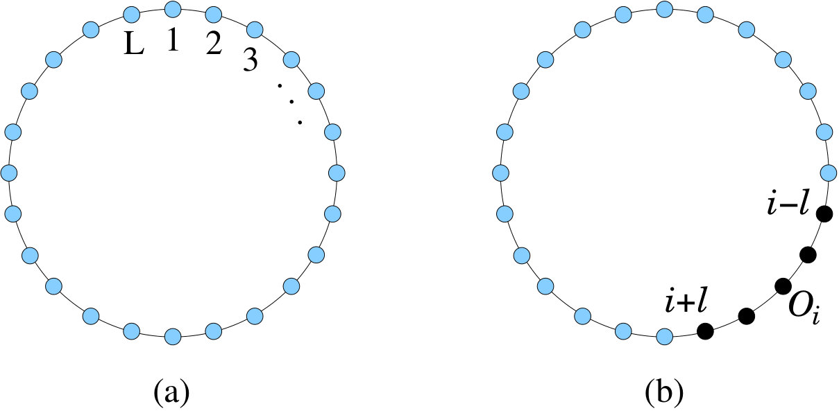 Figure 1
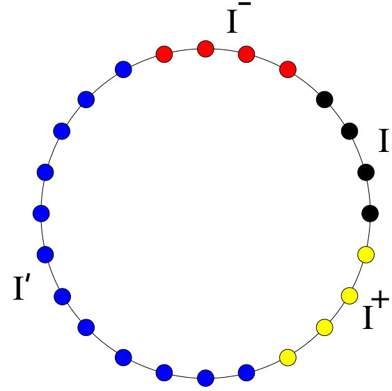 Figure 2
Peer Reviews
No public reviews on file for this paper yet. If you reviewed it on a platform where reviews are public (OpenReview, ICLR, NeurIPS, ICML), you can paste yours below so the community can read it here.
Videos
No videos yet. Explain this paper in a talk, walkthrough, or lecture? Add one.
Constraints on order and disorder parameters in quantum spin chains
Michael Levin Department of Physics, James Franck Institute, University of Chicago, Chicago, Illinois 60637, USA.
Abstract
We derive general constraints on order and disorder parameters in Ising symmetric spin chains. Our main result is a theorem showing that every gapped, translationally invariant, Ising symmetric spin chain has either a nonzero order parameter or a nonzero disorder parameter. We also prove two more constraints on order and disorder parameters: (i) it is not possible for a gapped, Ising symmetric spin chain to have both a nonzero order parameter and a nonzero disorder parameter; and (ii) it is not possible for a spin chain of this kind to have a nonzero disorder parameter that is odd under the symmetry. These constraints have an interesting implication for self-dual Ising symmetric spin chains: every self-dual spin chain is either gapless or has a degenerate ground state in the thermodynamic limit. All of these constraints generalize to spin chains without translational symmetry. Our proofs rely on previously known bounds on entanglement and correlations in one dimensional systems, as well as the Fuchs-van de Graaf inequality from quantum information theory.
Contents
1 Introduction
There are two distinct ways to probe symmetry breaking in quantum many-body systems. One approach is to use order parameters — local operators that transform under some non-trivial representation of the symmetry group. The other approach is to use disorder parameters — non-local operators that implement a symmetry transformation in some region, dressed with local operators along the boundary of the region[1]. These two approaches are complementary: while order parameters are useful for detecting symmetry breaking, disorder parameters are useful for detecting the absence of symmetry breaking.
The goal of this paper is to uncover the precise relationship between these two types of probes. To make progress, we focus on the simplest class of many-body systems in which order and disorder parameters can be defined: one dimensional quantum spin chains with Ising symmetry.
We begin by recalling the (rough) definitions of order and disorder parameters in the context of Ising symmetric spin chains. Consider a spin chain composed out of spin- moments. Suppose that the Hamiltonian commutes with the Ising symmetry transformation, . Such a spin chain has a nonzero “order parameter” if there exists an operator that is localized near site , is odd under (i.e. satisfies ), and obeys
[TABLE]
where denotes the ground state expectation value. Likewise, such a spin chain has a nonzero “disorder parameter” if there exists an operator that is localized near site , is either even or odd under (i.e. satisfies ), and obeys
[TABLE]
(Here, implements the Ising symmetry transformation within the interval ).
The canonical example is the transverse field Ising model:
[TABLE]
Depending on the value of , this model can be in two phases: a phase with spontaneously broken symmetry for , and a phase without symmetry breaking for . These two phases illustrate the concepts of order and disorder parameters. Indeed, a well-known property of the symmetry breaking phase is that . By the above definition, this property means that the symmetry breaking phase has a nonzero order parameter, namely . Likewise, a well-known property of the symmetric phase is that .111One way to derive this result is to note that the Kramers-Wannier duality transformation maps the operator to (see section 4). Following the above definition, this means that the symmetric phase has a nonzero disorder parameter, namely .
The above example raises the central question of this paper: we can see that the transverse field Ising model has either a nonzero order parameter or a nonzero disorder parameter for every except at the critical points . But is this true more generally? That is, does every gapped, translationally invariant, Ising symmetric spin chain have either a nonzero order parameter or a nonzero disorder parameter?
Conventional wisdom suggests that the answer is “yes.” The reasoning goes as follows: we expect that every spin chain of this kind can be adiabatically connected to the transverse field Ising model in either the symmetry breaking () or symmetric () phase[2, 3]. Therefore, since both phases of the transverse field Ising model have a nonzero order parameter or a nonzero disorder parameter, every gapped spin chain must also have this property[4].
In this paper, we confirm this intuition: we show that every gapped, translationally invariant, Ising symmetric spin chain has either a nonzero order parameter or a nonzero disorder parameter (Theorem 1). Our proof, however, does not follow the above line of reasoning, which is difficult to make rigorous. Instead, we derive a direct connection between order and disorder parameters using results from quantum information theory[5] together with bounds on correlations[6, 7] and entanglement[8] in one dimensional gapped ground states.
Our arguments also generalize to spin chains without translational symmetry. In that case, the statement of our theorem is slightly different since there is no reason that there has to be a nonzero order parameter or nonzero disorder parameter that is defined throughout the entire spin chain — parts of the spin chain may be ordered and other parts may be disordered. Thus, what we prove is that the spin chain can always be divided into a few regions, each of which supports either a nonzero order parameter or a nonzero disorder parameter (Theorem 2).
In addition to the above constraint (the main result of this paper), we also prove two other general constraints on order and disorder parameters: we show that (i) it is not possible for a gapped, Ising symmetric spin chain to have both a nonzero order parameter and a nonzero disorder parameter; and (ii) it is not possible for a spin chain of this kind to have a nonzero disorder parameter in which is odd under the symmetry (Theorems 3-4). All together, we believe that this is a complete list of constraints on order and disorder parameters in Ising symmetric spin chains.
As a bonus, our constraints have an interesting implication for self-dual spin chains that are invariant under the Kramers-Wannier duality transformation: they imply that every self-dual Ising symmetric spin chain is either gapless or has a degenerate ground state in the thermodynamic limit (Corollary 1).
What is our motivation for considering these questions? First, order and disorder parameters are key concepts in the theory of symmetry breaking in one dimension, and therefore we believe it is intrinsically important to understand their relationship to one another. In fact, it is possible to generalize order and disorder parameters to higher dimensional spin systems and gauge theories[1, 9] and one can ask similar questions in that context; the questions we consider here are the simplest examples of a larger class of problems.
Another source of motivation has to do with a seemingly unrelated problem about gapped boundaries of two dimensional topological phases. Previous work has argued that gapped boundaries of two dimensional Abelian topological phase always obey a property known as “braiding non-degeneracy”[10]. This property has important physical implications. For example, it is key for understanding why the boundaries of certain topological phases are necessarily gapless[10]. With Theorem 1, we can rigorously establish this property for the simplest nontrivial topological phase: the toric code model[11, 12]. This application will be explored in a follow-up paper[13].
This paper is organized as follows. In section 2, we discuss our main result: every gapped, translationally invariant, Ising symmetric spin chain has either a nonzero order parameter or a nonzero disorder parameter. In section 3 we present two other constraints on order and disorder parameters (namely constraints (i) and (ii) mentioned above) and in section 4 we discuss the implications of these constraints for self-dual spin chains. In sections 5 and 6 we present the proofs of our constraints.
2 Main result
Before stating our main result, we need to explain our setup. We consider spin chains made up of spins, arranged in a ring geometry (Fig. 1a). Each spin has possible states. We consider Hermitian Hamiltonians with nearest neighbor interactions and with bounded norm:
[TABLE]
We assume that is invariant under a (unitary) Ising symmetry transformation of the form
[TABLE]
where is a unitary operator acting on each -dimensional spin. Note that we do not sacrifice any generality in restricting to Hamiltonians with nearest-neighbor interactions: every one dimensional Hamiltonian with finite range interactions can be represented using nearest neighbor interactions by clustering sufficiently large groups of spins into superspins. Also note that we do not assume that is translationally invariant at this point.
A few comments about notation: (1) We denote the expectation value of the operator in the state by ; (2) We say that an operator is “even under ” if , and “odd under ” if . Likewise, we will say that a state in the spin-chain Hilbert space is “even under ” if , and “odd under ” if ; (3) We define the “distance” between sites in the obvious way: .
Next we define the notion of an order parameter — or more precisely a “ order parameter”:
Definition 1**.**
A collection of operators with is called a order parameter for a state , if
* is odd under .* 2. 2.
* is supported on .* 3. 3.
** 4. 4.
.
The set is called the domain of definition of the order parameter.
Here and are two positive real numbers that characterize different aspects of the order parameter: describes the size of the region of support of the operators (Fig. 1b) while describes the strength of the (two-point) correlations. Likewise, the subset should be thought of as the region where the order parameter is defined. In many cases, order parameters will be defined on the whole system, , but the above definition allows for the more general possibility where the order parameter is only defined on a subset of the system. This is particularly relevant to systems without translational symmetry.
Our definition for a disorder parameter is similar:
Definition 2**.**
A collection of operators is called a disorder parameter for a state if
The operators are all even under or all odd under . 2. 2.
* is supported on .* 3. 3.
** 4. 4.
.
The set is called the domain of definition of the disorder parameter.
Note that in the definition of disorder parameters, the operators are either all even or all odd. Thus we can distinguish between two types of disorder parameters: “even” and “odd” disorder parameters.
We are now ready to present our main result. Let be an Ising symmetric Hamiltonian of the form given in Eq. (1). The eigenstates of can always be chosen so that they have a definite parity — even or odd — under the Ising symmetry. In this paper, we focus on the even eigenstates.222Of course, all of our results also hold if we replace “even” by “odd.” Our results depend on a single assumption: the lowest energy eigenvalue within the even subspace is non-degenerate. We will denote the corresponding eigenstate by and the energy gap within the even subspace by . Our first result is that if is translationally invariant, then is guaranteed to have either a order parameter or a disorder parameter for appropriate and :
Theorem 1**.**
If is translationally invariant, then has either a order parameter or a disorder parameter defined on the whole spin chain (i.e. ) with
[TABLE]
(Here, and in the remainder of the paper, we use notation as follows: means that there exists constants and such that for all ).
A few comments about Theorem 1:
(1) It is important to recognize that the existence of a order/disorder parameter is only meaningful if is smaller than the system size . This means that the theorem does not give any meaningful constraints on gapless spin chains whose energy gaps scale like since in that case the bound on is larger than . On the other hand, the theorem does tell us something about gapped spin chains, i.e. spin chains where is bounded away from zero for arbitrarily large system sizes ; in this case, the theorem implies that there must be either an order parameter or a disorder parameter supported within a finite length scale that does not scale with the system size.
(2) The reader may worry that the theorem is inconsistent with the standard picture in which order/disorder parameters become arbitrarily small near critical points. The key point is that, unlike the standard setup, we do not fix a choice of order/disorder parameters across different Hamiltonians: these operators can change as we approach a critical point and, in particular, the region of support of these operators can grow (subject to the bound in Eq. 3) in order to maintain a fixed value of .
(3) To illustrate the theorem, consider the transverse field Ising model near the critical point. In this case, Theorem 1 implies that there exists either a order parameter or disorder parameter with and . It is interesting to compare this result to the usual renormalization group picture for the transverse field Ising model. Imagine we coarse grain the spin chain to a length scale of the same order as the correlation length . According to the renormalization group picture, we expect that the usual order and disorder parameters will have strength at this length scale. This suggests that we can always find an order or disorder parameter with and . Comparing with the above results, we see that Theorem 1 is consistent with the renormalization group picture and in fact the bounds on are weaker then one might expect. This suggests that it may be possible to strengthen these bounds further.
We now move on to the more general case where is not necessarily translationally invariant. In this case, the ground state can be spatially inhomogeneous so we may anticipate that the system can contain three types of regions: (1) regions that support an order parameter, (2) regions that support a disorder parameter that is even under , and (3) regions that support a disorder parameter that is odd under . The following theorem tells us that in fact, these three regions encompass the entire spin chain:
Theorem 2**.**
For general , there exists three sets with such that has a order parameter on , a disorder parameter that is even under on , and a disorder parameter that is odd under on . Here and .
Note that Theorem 2 is the natural generalization of Theorem 1: it shows that general spin chains can always be divided into three regions, each of which supports either an order parameter or a disorder parameter with definite parity.
3 Two more constraints on order and disorder parameters
In addition to the above results we also prove two more constraints on order and disorder parameters. These constraints do not simplify significantly in the translationally invariant case, so we will only state them in the general (non-translationally invariant) case. The first constraint is as follows:
Theorem 3**.**
If has a order parameter defined at two points and a disorder parameter defined at two points with , then
[TABLE]
To understand the implications of this result, consider the case where the order parameter and disorder parameter are defined throughout the entire spin chain, i.e. . In this case, we can choose to be equally spaced with a separation of . Then Eq. 4 implies
[TABLE]
This bound implies that is not possible for a spin chain to have both a order parameter and a disorder parameter defined throughout the whole chain and also have a finite gap in the limit . This is the constraint (i) mentioned in the introduction.
Our second constraint has a similar structure:
Theorem 4**.**
If has a disorder parameter that is odd under , defined at , then
[TABLE]
Again, the meaning of this constraint is most clear in the case where there is an odd disorder parameter that is defined throughout the entire spin chain. As above, if we choose to be equally spaced we derive the inequality (5). It then follows that it is not possible for a spin chain to have a disorder parameter that is odd under the symmetry and also have a finite gap in the limit . This is the constraint (ii) mentioned in the introduction.
Unlike Theorems 1-2, the proofs of Theorem 3 and 4 are straightforward: both theorems follow from the non-trivial commutation algebra obeyed by order and disorder parameters. In particular, Theorem 3 originates from the fact that order and disorder parameters anticommute, e.g. anticommutes with if . Likewise, Theorem 4 comes from the fact that odd disorder parameters obey a fermionic commutation algebra[14]. We present these proofs in section 6.
4 Application to self-dual spin chains
Our results have an interesting application to self-dual spin chains. Here we define the notion of self-dual spin chains as follows. Consider a spin- chain consisting of spins arranged in a ring, and consider a Hamiltonian of the form where and where each is supported on the interval for some integer , which we will refer to as the “range” of . Suppose further that commutes with the Ising symmetry . We say that is self-dual if where is the restriction of to the even () subspace and is the unitary operator, defined within the even subspace, given by
[TABLE]
The simplest example of a self-dual spin chain is the transverse field Ising model at .
Corollary 1**.**
For a self-dual spin chain with interactions of range , the energy gap within the even subspace is bounded by for every .
(Here, and in the rest of the paper, means that there exists a constant such that for all ).
This corollary implies that self-dual Ising symmetric spin chains cannot have a gapped, non-degenerate ground state (within the even subspace) in the thermodynamic limit .
Proof.
Let be the lowest energy even eigenstate. Given that the spin chain is self-dual we know that . To understand the implications of this, notice that the duality transformation maps order parameters onto even disorder parameters and vice-versa, e.g.
[TABLE]
It follows that if has a order parameter, then it also has an even disorder parameter and vice-versa.
Next observe that every self-dual Hamiltonian is translationally invariant since the square of the duality transformation acts like a unit translation on all even operators. This means that we can apply Theorem 1 which tells us that has either a order parameter or a disorder parameter with
[TABLE]
Here, the bound on comes from the fact that, in order to apply Theorem 1, we first need to cluster adjacent spin-’s into superspins of dimension in order to convert our spin chain into one with nearest neighbor interactions. In addition to clustering, we also have to multiply the resulting superspin Hamiltonian by in order to satisfy the norm condition (1); this leads to a gap of and explains the factor of in the denominator of (7).
Combining this observation with the previous one, we conclude that either (a) has both a order parameter and an even disorder parameter obeying (7) or (b) has an odd disorder parameter obeying (7). In the first case, Theorem 3 implies that where is the length of our spin chain after clustering together adjacent spin-’s into superspins. In the second case, we again deduce that — this time using Theorem 4.
The last step is to use the bound on (7), which gives the inequality . It then follows from our definition of that for every . Inverting this inequality gives the desired bound . ∎
5 Proof of main result
In this section, we prove Theorems 1 and 2. We begin with some definitions.
5.1 Definitions
First some notation: for each subset , let be the symmetry transformation restricted to , i.e.
[TABLE]
Next, we define a notion of when a state is “ strongly-ordered” on a pair of intervals :
Definition 3**.**
A state is strongly-ordered on disjoint intervals if there exist operators and such that:
* and are supported on and .* 2. 2.
* and are odd under .* 3. 3.
. 333We use the condition instead of for two reasons: (1) the first condition is simpler and (2) the two conditions are equivalent since one can replace . 4. 4.
.
We also define a notion of when a state is “ weakly-ordered” on a pair of intervals :
Definition 4**.**
A state is weakly-ordered on disjoint intervals if there exists an operator such that:
* is supported on .* 2. 2.
* is odd under and .* 3. 3.
. 4. 4.
.
To get some intuition about the above definition, notice that we can always expand as a linear combination where are operators supported on . The second condition then amounts to the requirement that and are odd under for all . Likewise, the third condition becomes . From this point of view, we can see that the main difference between weak order and strong order is that the former characterizes the correlations that can be detected by entangled operators of the form , while the latter characterizes the correlations that can be detected by simple products .
We define the notion of strong disorder and weak disorder in a similar fashion:
Definition 5**.**
A state is strongly-disordered on disjoint, non-adjacent intervals if there exist operators and such that
* and are supported on and .* 2. 2.
* and are both even or both odd under .* 3. 3.
* where is the interval between and , going clockwise.* 4. 4.
.
Notice that are either both even or both odd under : in the former case, we will say that is strongly-disordered with even parity, while in the latter case we will say that is strongly-disordered with odd parity.
Definition 6**.**
A state is weakly-disordered on disjoint, non-adjacent intervals if there exists an operator such that
* is supported on .* 2. 2.
* is even under both or odd under both .* 3. 3.
* where is the interval between and , going clockwise.* 4. 4.
.
Similarly to above, we will say that is weakly-disordered with even or odd parity depending on whether is even or odd under .
5.2 Main argument
Before giving the proof of Theorems 1-2, we need to introduce one last piece of notation: given an interval we define and to be the two intervals that are adjacent to and have the same length as (see Fig. 2). Also, we define to be the interval
[TABLE]
Proof.
(of Theorems 1 and 2) We start by proving Theorem 2: we show that there exists three sets with , such that has a order parameter on , a disorder parameter that is even under on , and a disorder parameter that is odd under on .
We proceed in three steps — each of which depends on an associated lemma. We give the proofs of these lemmas in the next section. The first lemma is a quantum information theory result that applies to any state that has a definite parity under :
Lemma 1**.**
Let be a state that is even or odd under . For every pair of disjoint, non-adjacent intervals , the state is either weakly-ordered on or weakly-disordered on the complementary intervals , where the intervals are ordered , going clockwise.
Lemma 1 is useful because it gives a way to construct the three sets , and . Fix an integer , to be chosen later, and for each , define . We claim that the state is either weakly-ordered on or weakly-disordered on for each . To see this, apply Lemma 1 to the two intervals with . The lemma tells us that is either weakly-ordered on or weakly-disordered on the complementary intervals . This implies our claim since every state that is weakly-disordered on is also weakly disordered on since . We now define:
[TABLE]
By construction, . To proceed further, we invoke the following lemma:
Lemma 2**.**
For every , there exists a length444Here, we treat as a constant when using notation. such that if is weakly-ordered on then it is strongly-ordered on for all that are separated by a distance of at least . Likewise, if is weakly-disordered on with even (odd) parity then it is strongly-disordered on with even (odd) parity for all separated by at least .
Lemma 2 is important because it allows us to upgrade from weak order/disorder to strong order/disorder. This upgrade, in turn, allows us to construct order and disorder parameters. To construct an order parameter, we apply the above lemma with . We then choose to be larger than the length given in the above lemma. With this choice of , it follows that is strongly-ordered on for each . This means that, for each , there exists operators supported on that are odd under the symmetry and satisfy . We define our order parameter to be the corresponding operators: . Likewise, to construct disorder parameters, we use the lemma to deduce that, for each (), there exists operators supported on that are even (odd) under the symmetry and satisfy . We define the disorder parameters on to be the corresponding operators: and .
All that remains is to show that the above order and disorder parameters have long range correlations. We do this with the help of the following lemma:
Lemma 3**.**
Let be two disjoint intervals and let . For any operators supported on that are all odd or all even under and have norm of at most ,
[TABLE]
where for some , and denotes the interval between and (going clockwise).
To apply Lemma 3, consider any with . Then, it is easy to see that
[TABLE]
Therefore the inequality (9), with and gives
[TABLE]
Using , we deduce that
[TABLE]
By the same reasoning, the inequality (10) implies that
[TABLE]
for every or with .
The last step is to note that above expression for implies that there exists , such that for . Therefore, if we choose , then we have
[TABLE]
At this point we have constructed a order parameter on , and a disorder parameter on and with and . This establishes Theorem 2.
The proof of Theorem 1 is almost exactly the same: the only change in this case is that translational symmetry guarantees that and and must either be empty sets or the full set . This means that at least one of , or , so has either a order parameter or disorder parameter defined on the whole system, as claimed. ∎
5.3 The Fuchs-van de Graaf inequality and the proof of Lemma 1
In this section, we prove Lemma 1. At the heart of the proof is the following general inequality from quantum information theory. Consider any two spin states and any collection of spins, . Then:
[TABLE]
Here the first maximum is over all operators that have and are supported in , and the second maximum is over all unitary operators that are supported in . Intuitively, the first term in Eq. (11) measures how distinguishable are with respect to observables in , while the second term measures to what extent can be transformed into by a unitary operation in . Thus, (11) tells us that if two states look similar with respect to measurements in , then it must be possible to (approximately) transform one state into the other with an operation in .
The inequality (11) is easiest to prove in the limiting case where the first term is exactly zero: i.e. for every supported in . In this case, and have identical reduced density matrices in the region . It then follows that there exists a unitary operator , supported in , such that : indeed, the operator that does the job is the unitary transformation that rotates the Schmidt states for in the region into the corresponding Schmidt states for .
To derive the inequality (11) in the general case, let be the reduced density matrices of in the region . The first term in Eq. (11) is then equal to the trace distance between , usually denoted by . Likewise, the second term in Eq. (11) can be identified with the square root of the fidelity, , using Uhlmann’s theorem[15]. With these identifications, Eq. (11) is an immediate consequence of the Fuchs-van de Graaf inequality[5]: .
With the inequality (11) in hand, we are now ready to prove Lemma 1:
Lemma 1.
Let be a state that is even or odd under . For every pair of disjoint, non-adjacent intervals , the state is either weakly-ordered on or weakly-disordered on the complementary intervals , where the intervals are ordered going clockwise.
Proof.
Let , and . Substituting this into (11) gives
[TABLE]
An obvious consequence of Eq. (12) is that either:
- (i)
The first term is larger than . 2. (ii)
The second term is larger than .
We claim that in case (i), is weakly ordered on , while in case (ii), is weakly disordered on . Indeed, in case (i), define
[TABLE]
where is the maximal choice of . By assumption, . Furthermore, it is easy to see that is supported on , is odd under and has norm of at most . It follows that is weakly ordered on . In case (ii), define
[TABLE]
where is the maximal choice of . By assumption, . Hence either or . Furthermore, it is easy to see that are supported on , are even/odd under , and have norm of at most . It follows that is weakly disordered on . ∎
5.4 Some bounds on correlations and the proof of Lemma 3
We now give the proof of Lemma 3. One of the key tools in our proof is a general result about the factorizability of gapped ground states. This result was first proven by Hastings[6] and subsequently generalized in Ref. [7]. Here we adapt this result to the case of interest, namely Ising symmetric Hamiltonians in a ring geometry:
Theorem 5**.**
(Hastings)* Let be the lowest energy even eigenstate of an Ising symmetric Hamiltonian (1). Then for every interval and every there exists a corresponding Hermitian projection operator that is supported on , is even under , and has the following property: given a partition of into four intervals , there exists an operator with , that is supported in the region X_{bd}=\{i:\text{dist}(i,I_{n})<\ell/2,\text{for at least two different n's}\} and that is even under for every connected component of , such that*
[TABLE]
where is a numerical constant, is the energy gap within the even subspace, and is the projection onto the even subspace.
Proof.
There are only three small differences between Theorem 5 and Hastings’ original result (Lemma 1 from Ref. [6]): First, Theorem 5 applies to Ising symmetric Hamiltonians that have a gap within the even subspace while Lemma 1 from Ref. [6] applies to generic Hamiltonians that have a gap within the full Hilbert space. Second, Theorem 5 applies to spin chains with a ring geometry while Lemma 1 from Ref. [6] applies to spin chains with open boundary conditions. Finally, Theorem 5 applies to a partition into four intervals while Lemma 1 from Ref. [6] applies to a partition into two intervals. The first difference has only a minor effect on the proof — all arguments go through exactly as in Ref. [6], with the only modification being that one needs to multiply the right hand side of Eq. (A.6) in Ref. [6] by the projector ; this is carried through to all subsequent equations, including the final result (A.11). The claim that can be chosen to be even under for every connected component of follows from the fact that the operator appearing in Eq. (A.10) can be written as a sum, , where is even under and is supported on . The second and third differences are even more trivial: it is not hard to see that the proof given in Ref. [6] works equally well for a ring geometry and for a partition into any finite number of intervals. ∎
We now use the above theorem to prove three propositions. The first proposition essentially says that the operators defined above can be used as (approximate) ground state projection operators in appropriate circumstances:
Proposition 1**.**
(Gd. state projectors)* Let be an operator that is even under , has norm of at most and is supported on where are two intervals separated by a distance of at least . Then,*
[TABLE]
where and denotes the interval between and (going clockwise).
Proof.
We will start with (14). Let and be the two intervals that make up . Then define a partition of into four intervals. Therefore Theorem 5 implies that
[TABLE]
Multiplying this equation by , and dropping the ’s for notational simplicity, we derive:
[TABLE]
Reordering the terms, using the fact that commute with , gives
[TABLE]
At the same time, Eq. 16 implies that
[TABLE]
Indeed, this follows from the following claim[16]:
Claim 1**.**
Suppose that where is a projector and . Then:
[TABLE]
For example, to derive the first equation in (18), set and , and . The other equations follow in a similar manner.
Proof.
(of Claim 1) Note that the Cauchy-Schwarz inequality implies
[TABLE]
It follows that . At the same time, the following inequality holds for any vectors with norm at most :
[TABLE]
Applying this inequality to , we derive
[TABLE]
This establishes (19). Likewise, applying (21) to , we deduce that
[TABLE]
By the triangle inequality,
[TABLE]
This establishes (20). ∎
If we now combine (17) and (18), we deduce that
[TABLE]
This completes our derivation of (14). As for (15), note that Theorem 5 implies that
[TABLE]
Similarly to before, reordering the terms gives
[TABLE]
By the same reasoning as above, Eq. 18 implies the desired inequality:
[TABLE]
∎
We now move on to the second proposition — a variation of Hastings’ result that gapped ground states have short range correlations[17]:
Proposition 2**.**
(Short-range correlations)* Let be two operators that are even under the symmetry, have norm of at most and are supported on intervals separated by a distance of at least . Then,*
[TABLE]
Proof.
By construction, define a partition of into two intervals. Therefore, according to Theorem 5 (with and being empty sets),
[TABLE]
Sandwiching this inequality between and gives
[TABLE]
where we have dropped the ’s for clarity. Reordering the terms, we obtain
[TABLE]
where we have used the fact that commutes with and commutes with .
At the same time, using (24) and Claim 1, we deduce
[TABLE]
Combining (25) and (26) gives:
[TABLE]
This implies the desired inequality (23). ∎
Our final proposition is also a result about short-range correlations, but in the more complicated case where the operators in question are either odd under symmetry or involve a symmetry transformation along an interval:
Proposition 3**.**
(Generalized short-range corr.)* For any intervals separated by a distance of at least , there exists three pairs of operators , , supported on with*
[TABLE]
where Eqs. (27) and (29) hold for every that are supported on , are odd under , and have norm of at most , and Eq. (28) holds for every that are supported on , are even under , and have norm of at most . Here, is a constant, and is the interval between (going clockwise).
Proof.
We start with Eq. (27). To derive this result, define and let
[TABLE]
Also, let be any two operators that are supported on , are odd under and have norm of at most . We claim that the following inequalities hold:
[TABLE]
Here the first inequality follows from Proposition 1, while the second inequality follows from the fact that has short-range correlations (Proposition 2) and that and are supported on two intervals that are separated by a distance of at least .
Adding together these two inequalities and using the triangle inequality, we derive
[TABLE]
Now, let us choose such that is as large as possible. There are two cases to consider: or . In the first case, Eq. (27) holds with and . In the second case, we can divide (30) by to obtain
[TABLE]
with
[TABLE]
Again this establishes the desired inequality, Eq. (27), with .
The proof of Eq. (28) is similar. In this case, let be any two operators that are supported on , are even under and have norm of at most . We claim that the following inequalities hold:
[TABLE]
As above, the first inequality follows from Proposition 1, while the second inequality follows from the fact that has short-range correlations (Proposition 2).
Adding together these three inequalities, we derive
[TABLE]
As above, we now choose such that is as large as possible. If , then Eq. (28) holds with . On the other hand, if , then we can divide (31) by to obtain
[TABLE]
with
[TABLE]
This gives the desired inequality, Eq. (28), with . The proof of Eq. (29) follows in exactly the same way.
∎
We are now ready to prove Lemma 3:
Lemma 3.
Let be two disjoint intervals and let . For any operators supported on that are all odd or all even under and have norm of at most ,
[TABLE]
where for some , and denotes the interval between and (going clockwise).
Proof.
We begin with (32). Let and
[TABLE]
The proof proceeds in three steps. First, we note that and are supported on two intervals which are separated by a distance of at least . Therefore Proposition 2 implies
[TABLE]
It follows that
[TABLE]
Next observe that and since
. Substituting these inequalities into (34), we conclude that
[TABLE]
Next we invoke Proposition 1 which implies that
[TABLE]
Combining (35),(36), we derive:
[TABLE]
This establishes the desired inequality (32) with .
The derivation of (33) is similar: first we note that
[TABLE]
by the same reasoning as in (34). Next we observe that
[TABLE]
where the first equality follows from and similarly for the second equality. Also, we have the inequalities
[TABLE]
Putting this together gives:
[TABLE]
Next, we invoke Proposition 1 to deduce
[TABLE]
Combining (37), (38), we derive
[TABLE]
This establishes the desired inequality (33) with . ∎
5.5 A bound on entanglement and the proof of Lemma 2
In this section we prove Lemma 2. The key tool in our proof is a bound on entanglement in gapped ground states due to Arad, Kitaev, Landau, and Vazirani [8]. Here we adapt this bound to the case of Ising symmetric Hamiltonians:
Theorem 6**.**
(AKLV)* Let be the lowest energy even eigenstate of an Ising symmetric Hamiltonian (1) and let be the energy gap in the even subspace. Then for every bipartition of the spin chain into two intervals, and every , there exists an even state with overlap and with a Schmidt rank across the cut of at most .555Here we treat as a constant when using notation.*
Proof.
There are only two small differences between Theorem 6 and the original result of Arad, Kitaev, Landau, and Vazirani (Lemma 6.3 from Ref. [8]): first, Theorem 6 applies to Ising symmetric Hamiltonians that have a gap within the even subspace, while Lemma 6.3 from Ref. [8] applies to generic Hamiltonians with a gap within the full Hilbert space. Second, Theorem 6 applies to spin chains in a ring geometry while Lemma 6.3 from Ref. [8] applies to spin chains with open boundary conditions. The first modification does not affect the proof in any way: the approximate ground state projector (AGSP) constructed in Ref. [8] is guaranteed to be Ising symmetric as long as the Hamiltonian is, so the same arguments go through in the Ising symmetric case as in Lemma 6.3 in Ref. [8]. The second modification can also be accommodated trivially since any spin chain in a ring geometry can be rewritten as a spin chain with open boundary conditions, by “squashing” the ring — that is, clustering pairs of spins into a single superspin with dimension . ∎
We now proceed with the proof of Lemma 2:
Lemma 2.
For every , there exists a length such that if is weakly-ordered on then it is strongly-ordered on for all that are separated by a distance of at least . Likewise, if is weakly-disordered on with even (odd) parity then it is strongly-disordered on with even (odd) parity for all separated by at least .
Proof.
We begin with the first part of the Lemma. Suppose that is weakly ordered on . We wish to show that it is strongly ordered on as long as are separated by a sufficiently large distance. The first step is to invoke Theorem 6 to construct a state that has a Schmidt rank for the bipartition and that has an overlap . For the moment, we leave undetermined — we will choose a specific value later.
By definition, we can Schmidt decompose using at most Schmidt states:
[TABLE]
Here are the Schmidt basis states corresponding to the region , and are the Schmidt states in region , ordered in such a way that the Schmidt coefficients vanish for .
Now since is weakly ordered on , there exists an operator supported on that is odd under and and satisfies . Like any operator acting on we can decompose into a sum
[TABLE]
where and where the are some (undetermined) operators acting on . Since , we must have . Also, since is odd under and , we know that are odd under the symmetry for all the nonvanishing terms in (39).
Now consider the expectation value . It is clear from the expression for that the only terms in (39) that contribute are those with , so that
[TABLE]
At the same time, the formula for the trace distance between pure states implies that
[TABLE]
(In the second equation we use which follows from the fact that where ). Combining these three equations with the fact that , implies the lower bound
[TABLE]
Next we invoke Proposition 3. In particular, we use Eq. (27) to deduce that
[TABLE]
since is a sum of terms, each of the form .
To proceed further, consider the problem of maximizing the quantity subject to the constraint that is supported on , is odd under and , and has norm at most . Given that is a tensor product of two operators supported on it is easy to see that the maximal choice of is a product of the form where are supported on , are odd under the symmetry, and have norm of at most .666In fact, one can derive an explicit formula for : the operator where is the unitary operator appearing in the polar decomposition of . In particular, this means that
[TABLE]
At the same time, we can apply Eq. (27) again to derive the inequality
[TABLE]
We now combine the four inequalities (40), (41), (42), (43) to conclude that
[TABLE]
The last step is to choose so that . The inequality then becomes
[TABLE]
Finally, comparing the expressions for and , we see that there exists such that if then and hence . This proves the first part of the Lemma.
To prove the second part, we use the same logic. Suppose that is weakly disordered with even parity. Then there exists an operator supported on that is even under and satisfies . As above, we can approximate by a state with overlap and Schmidt rank for the bipartition . Decomposing and in the same way as above, we have
[TABLE]
where are both even under and have norm at most . Following the same logic as before gives the lower bound
[TABLE]
Next we apply the above proposition to derive the inequality
[TABLE]
In the same way as before we have
[TABLE]
for some that are supported on , are even under the symmetry, and have norm of at most . Also,
[TABLE]
Putting this all together gives
[TABLE]
Choosing as before gives the desired inequality for . Exactly the same argument works when is weakly disordered with odd parity. ∎
6 Proofs of additional constraints
In this section, we present the proofs of the two additional constraints on order and disorder parameters: Theorems 3 and 4.
Theorem 3.
If has a order parameter defined at two points and a disorder parameter defined at two points with , then
[TABLE]
Proof.
Let and be the postulated order and disorder parameters, respectively. Without loss of generality, we can assume that
[TABLE]
since we can always make these equalities hold by replacing for appropriate . Let and define
[TABLE]
where
[TABLE]
and where and . Then according to Proposition 1,
[TABLE]
It follows that
[TABLE]
Likewise,
[TABLE]
At the same time, and anti-commute:
[TABLE]
Indeed, this follows immediately from the fact that is odd under the symmetry . Combining (45)-(47), we deduce that
[TABLE]
Plugging in the expression for gives the desired inequality: . ∎
Theorem 4.
If has a disorder parameter that is odd under , defined at , then
[TABLE]
Proof.
Let be the postulated disorder parameters. As before, we can assume without loss of generality that
[TABLE]
Let and define
[TABLE]
where are defined in the same way as in (44). Then according to Proposition 1,
[TABLE]
It follows that
[TABLE]
Likewise,
[TABLE]
At the same time, it is not hard to see that obey the “fermionic” commutation algebra[14]
[TABLE]
To see this, note that
[TABLE]
where the minus sign comes from the fact that is odd under . Combining (48)-(50), we deduce that
[TABLE]
Plugging in the expression for gives the desired inequality: . ∎
7 Discussion
This work could potentially be extended in several directions. The simplest extension would be to consider spin chains with more general symmetry groups. In particular, we expect that all of our results (Theorems 1-4) can be easily generalized to arbitrary finite, Abelian symmetry groups. Non-abelian symmetries are more challenging and would be an interesting direction for future work.
Another natural extension would be to consider spin chains whose symmetry transformations are not onsite, i.e. not a product of single spin unitaries. (For an example, see the Ising symmetry transformation given in Ref. [18]). Results about such spin chains would be relevant to the edge physics of two dimensional symmetry protected topological phases.
Finally, one could consider higher dimensional spin systems. We do not know whether Theorem 1, which guarantees the existence of order or disorder parameters in gapped, translationally invariant spin chains, has an analog in higher dimensions. However, Theorem 2, which guarantees a similar result in the non-translationally invariant case, is unlikely to have such a generalization. Indeed, the phenomenon of weak symmetry breaking[19] shows that there exist two dimensional gapped systems with broken symmetries whose order parameters are non-local. These systems do not support either a disorder parameter or a local order parameter anywhere in the weak symmetry breaking region so they provide counterexamples to higher dimensional analogs of Theorem 2.
8 Acknowledgments
I would like to thank Maxim Zelenko for pointing out a gap in the proof of Proposition 1 in a previous draft of this paper and the need for a slightly stronger version of Theorem 5. This work was supported in part by the NSF under grant No. DMR-1254741.
The reference list from the paper itself. Each links out to its DOI / PubMed record.
- 1[1] E. Fradkin, Disorder operators and their descendants , J. Stat. Phys. 167 , p. 427 (2017).
- 2[2] N. Schuch, D. Perez-Garcia, and I. Cirac, Classifying quantum phases using matrix product states and projected entangled pair states , Phys. Rev. B 84 , 165139 (2011).
- 3[3] X. Chen, Z.-C. Gu, and X.-G. Wen, Complete classification of one-dimensional gapped quantum phases in interacting spin systems , Phys. Rev. B 84 , 235128 (2011).
- 4[4] M. B. Hastings and X.-G. Wen, Quasiadiabatic continuation of quantum states: The stability of topological ground-state degeneracy and emergent gauge invariance , Phys. Rev. B 72 , 045141 (2005).
- 5[5] C. Fuchs and J. van de Graaf, Cryptographic distinguishability measures for quantum-mechanical states , IEEE Trans. Inform. Theory 45 , p. 1216 (1999).
- 6[6] M. B. Hastings, An area law for one-dimensional quantum systems , J. Stat. Mech. Theory Exp. 2007 , p. 8024 (2007).
- 7[7] E. Hamza, S. Michalakis, B. Nachtergaele, and R. Sims, Approximating the ground state of gapped quantum spin systems , J. Math. Phys. 50 , 095213 (2009).
- 8[8] I. Arad, A. Kitaev, Z. Landau, and U. Vazirani, An area law and sub-exponential algorithm for 1D systems , ar Xiv:1301.1162.