Regularity and Koszul property of symbolic powers of monomial ideals
Le Xuan Dung, Truong Thi Hien, Hop D. Nguyen, Tran Nam Trung

TL;DR
This paper investigates the asymptotic behavior of regularity and generating degrees of symbolic powers of monomial ideals, revealing convergence properties and introducing new methods for analyzing componentwise linearity.
Contribution
It demonstrates the convergence of normalized regularity and generating degree sequences and introduces a novel approach to establish componentwise linearity of symbolic powers.
Findings
Sequences of regularity and generating degrees converge to the same limit.
Existence of monomial ideals where these functions are not eventually linear.
New method for proving componentwise linearity of symbolic powers.
Abstract
Let be a homogeneous ideal in a polynomial ring over a field. Let be the -th symbolic power of . Motivated by results about ordinary powers of , we study the asymptotic behavior of the regularity function and the maximal generating degree function , when is a monomial ideal. It is known that both functions are eventually quasi-linear. We show that, in addition, the sequences and converge to the same limit, which can be described combinatorially. We construct an example of an equidimensional, height two squarefree monomial ideal for which and are not eventually linear functions. For the last goal, we introduce a new method for establishing the componentwise linearity of ideals. This method allows us to identify a new…
Click any figure to enlarge with its caption.
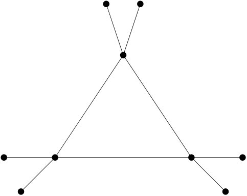 Figure 1
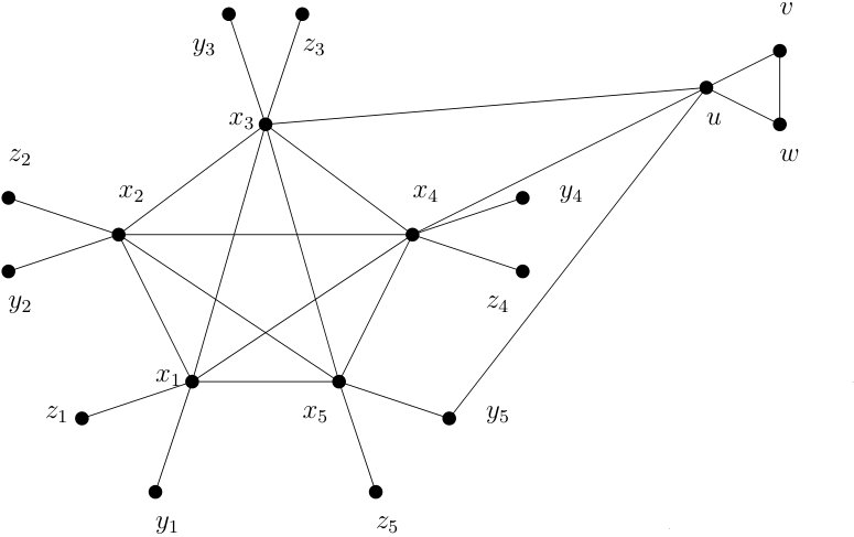 Figure 2
Peer Reviews
No public reviews on file for this paper yet. If you reviewed it on a platform where reviews are public (OpenReview, ICLR, NeurIPS, ICML), you can paste yours below so the community can read it here.
Videos
No videos yet. Explain this paper in a talk, walkthrough, or lecture? Add one.
Regularity and Koszul property of symbolic powers of monomial ideals
Le Xuan Dung
Faculty of Natural Sciences, Hong Duc University No. 565 Quang Trung, Dong Ve, Thanh Hoa, Vietnam
,
Truong Thi Hien
Faculty of Natural Sciences, Hong Duc University No. 565 Quang Trung, Dong Ve, Thanh Hoa, Vietnam
,
Hop D. Nguyen
Institute of Mathematics, VAST, 18 Hoang Quoc Viet, Hanoi, Viet Nam
and
Tran Nam Trung
Institute of Mathematics, VAST, 18 Hoang Quoc Viet, Hanoi, Viet Nam, and TIMAS, Thang Long University, Ha Noi, Vietnam.
Abstract.
Let be a homogeneous ideal in a polynomial ring over a field. Let be the -th symbolic power of . Motivated by results about ordinary powers of , we study the asymptotic behavior of the regularity function and the maximal generating degree function , when is a monomial ideal. It is known that both functions are eventually quasi-linear. We show that, in addition, the sequences and converge to the same limit, which can be described combinatorially. We construct an example of an equidimensional, height two squarefree monomial ideal for which and are not eventually linear functions. For the last goal, we introduce a new method for establishing the componentwise linearity of ideals. This method allows us to identify a new class of monomial ideals whose symbolic powers are componentwise linear.
Key words and phrases:
Castelnuovo-Mumford regularity, symbolic power, componentwise linear, Koszul module, cover ideal
2010 Mathematics Subject Classification:
13D02, 05C90, 05E40, 05E45.
1. Introduction
Let be a polynomial ring over a field . In this paper we investigate the maximal generating degree and the regularity of symbolic powers of monomial ideals in . Let be a homogeneous ideal of . Then the -th symbolic power of is defined by
[TABLE]
where is as usual the set of minimal associated prime ideals of .
Symbolic powers were studied by many authors. While sharing some similar features with ordinary powers, the symbolic powers are usually much harder to deal with. One difficulty lies in the fact that the symbolic Rees algebra, defined as
[TABLE]
is not noetherian in general. Examples of non-noetherian symbolic Rees algebras were discovered by Roberts [32] and simpler examples were provided by Goto-Nishida-Watanabe [11].
Denote by and to be the regularity of and the maximal degree of the minimal homogeneous generators , respectively. By celebrated results by Cutkosky-Herzog-Trung [7] and Kodiyalam [23], we know that and are eventually linear functions with the same leading coefficient. In particular, there exist the limits
[TABLE]
and the common limit is an integer. On the other hand, by [3, Proposition 7], when defines points on a rational normal curve in , where , then for all ,
[TABLE]
Hence the function is not eventually linear in general. Cutkosky [6] could even construct a smooth curve in whose homogeneous defining ideal has the property that is an irrational number. Another peculiar example is given in [7, Example 4.4]: given any prime number modulo 3, there exist some field of characteristic , and some collection of 17 fat points in whose defining ideal has the property that is not eventually quasi-linear.
While the question about eventual quasi-linear behavior of has a negative answer in general, various basic questions remain tantalizing. For example:
- (1)
There was no known example of a homogeneous ideal in a polynomial ring for which the limit does not exist (Herzog-Hoa-Trung [18, Question 2]); 2. (2)
It remains an open question whether for every such homogeneous ideal , the function is bounded by a linear function; 3. (3)
Even an answer for the analogue of the last question for remains unknown.
In [21, Theorem 4.9], it is shown that exists if is a squarefree monomial ideal (but a description of the limit was not provided). By [18, Section 2], Question (2) (and hence of course (3)) has a positive answer if either is a monomial ideal, or , or the singular locus of has dimension at most 1. The general case remains open for all of these questions.
Symbolic powers of monomial ideals are simpler than that of general ideals because symbolic Rees algebras of monomial ideals are noetherian [24, Proposition 1], [17, Theorem 3.2]. In the present paper, we address the following questions for a monomial ideal of .
Question 1.1**.**
Does the limit exist? If it does, describe the limit in terms of . The same questions for .
Question 1.2** (Minh-T.N. Trung [26, Question A, part (i)]).**
Is the function eventually linear if is squarefree?
A motivation for Question 1.2 is a result of Herzog, Hibi, Trung [17], that is eventually quasi-linear. Another motivation is a recent result of Hoa et al. [20] on the existence of when is a squarefree monomial ideal. It is worth pointing out that Question 1.2 has a negative answer for non-squarefree monomial ideals; see Example 3.10.
Extending previous result of Hoa and T.N. Trung, our first main result answers Question 1.1 in the positive for both limits (they are actually the same). We also describe explicitly the limits in terms of certain polyhedron associated to . Our second main result answers the other question in the negative. In fact, a counterexample is given using equidimensional height 2 squarefree monomial ideals, in other words, cover ideals of graphs. Interestingly, at the same time, our counterexample also gives a negative answer for the analogue of Question 1.2 for the function .
In detail, the main tool for Question 1.1 comes from the theory of convex polyhedra. Assume that admits a minimal primary decomposition
[TABLE]
where are all the primary monomial ideals associated to the minimal prime ideals of . We define certain polyhedron associated to as follows:
[TABLE]
where is the Newton polyhedron of . Then is a convex polyhedron in . For a vector , denote . Let
[TABLE]
Answering Question 1.1, our first two main results are:
Theorem 1.3** (Theorems 3.3 and 3.6).**
For all monomial ideals , there are equalities
[TABLE]
While computing the regularity of the symbolic powers of it is difficult, the computation of is fairly simple by linear programming technique.
It is not hard to show that if is a squarefree monomial ideal (Lemma 4.3). Moreover, there are many examples in which . This is the case when is a quadratic squarefree monomial ideal (hence ), thanks to a result by Bahiano [2]; see Example 4.4. Let be an arbitrary simple graph with the vertex set and the edge set . Recall that the cover ideal of is defined by
[TABLE]
We also prove in Theorem 4.9 that , if is either bipartite, unmixed, or claw-free. An exact formula for remains elusive even for such graphs; see, for example, [36, 37], for related work. Proposition 4.11 provides another large class of graphs for which the equality holds. Our main tool for proving Theorem 4.9 and Proposition 4.11 is a combinatorial formula for in Theorem 4.6. It looks challenging to interpret in terms of other known graph-theoretical invariants of .
We next study componentwise linear ideals in the sense of Herzog and Hibi [14] which are also known as Koszul ideals [19]. Our main tool is the following new result on Koszul ideals, which is proved by the theory of linearity defect.
Proposition 1.4** (See Theorem 5.1).**
Let be a polynomial ring over with the graded maximal ideal . Let be a non-zero linear form, and non-zero homogeneous ideals of such that the following conditions are simultaneously satisfied:
- (i)
* is Koszul;* 2. (ii)
; 3. (iii)
* is a regular element with respect to and , the associated graded module of with respect to the -adic filtration.*
Denote . Then is Koszul if and only if is so.
A common method (among a dozen of others), to establish the Koszul property of an ideal is to show that it has linear quotients. Compared with this method, the criterion of Proposition 1.4 has the advantage that it does not require the knowledge of a system of generators of the ideal. It just asks for the knowledge of a decomposition which is in many cases not hard to obtain, the more so if we work with monomial ideals. Indeed, let be a monomial ideal of , and one of its variables. Then we always have a decomposition , where are monomial ideals, and does not divide any minimal generator of . For such a decomposition, condition (iii) in Proposition 1.4 is automatic. Hence given conditions (i) and (ii), we can prove the Koszulness of by passing to , which lives in a smaller polynomial ring.
Proposition 1.4 is interesting in its own and has further applications, which we hope to pursue in future work. The main application of this proposition in our paper is to study the Koszulness of symbolic powers of the cover ideal of a graph . By using Proposition 1.4, we prove:
Theorem 1.5** (Theorem 5.7).**
Let be the graph obtained by adding to each vertex of a graph at least one pendant. Then all the symbolic powers of are Koszul.
It is worth mentioning that, via Alexander duality, this can be seen as a generalization of previous work of Villarreal [41] and Francisco-Hà [9] on the Cohen-Macaulay property of graphs.
In order to give a counter-example to Question 1.2, we apply Theorem 1.5 for corona graphs.
Theorem 1.6** (Theorem 5.15).**
For and , let be the graph obtained from the complete graph on vertices by adding exactly pendants to each of its vertex. Let . Then for all ,
- (1)
; 2. (2)
.
In particular, for all ,
[TABLE]
which is not an eventually linear function of .
Let us summarize the structure of this article. In Section 2, we recall some necessary background. In Section 3, we prove that for any monomial ideal , the limits and exist and equal to each other. We identify them in terms of the afore-mentioned polyhedron associated to . In Section 4, we describe structural properties of the symbolic powers of a cover ideal , and compute the function in terms of the graph in certain situations. We are able to show that for graphs which are either bipartite, unmixed, or claw-free (Theorem 4.9). In Section 5, we first prove the Koszulness criterion of Proposition 1.4. The main result of this section is the Koszul property of the symbolic powers for certain class of cover ideals, stated in Theorem 5.7. Combining this with results in Section 4, Theorem 1.6 is deduced at the end of this section.
2. Preliminaries
For standard terminology and results in commutative algebra, we refer to the book of Eisenbud [8]. Good references for algebraic aspects of monomial ideals and simplicial complexes are the books of Herzog and Hibi [15], Miller and Sturmfels [25], and Villarreal [42].
2.1. Regularity
Let be a standard graded algebra over a field . Let be a finitely generated graded nonzero -module. Let
[TABLE]
be the minimal graded free resolution of over . For each , , denote and . We usually omit the superscript and write simply and whenever this is possible. Let
[TABLE]
where, by convention, if . The Castelnuovo–Mumford regularity of measures the growth of the generating degrees of the , . Concretely, it is defined by
[TABLE]
In the remaining of this paper, we denote by the number . Hence is the maximal degree of a minimal homogeneous generator of . The definition of the regularity implies
[TABLE]
If is generated by elements of the same degree , and , we say that has a linear resolution over . We also say has a -linear resolution in this case.
If is a standard graded polynomial ring over , it is customary to denote simply by .
2.2. Linearity defect, Koszul modules, Betti splittings
We use the notion of linearity defect, formally introduced by Herzog and Iyengar [19]. Let be a standard graded -algebra, and a finitely generated graded -module. The linearity defect of over , denoted by , is defined via certain filtration of the minimal graded free resolution of . For details of this construction, we refer to [19, Section 1]. We say is called a Koszul module if . Koszul modules are those modules with a linear resolution in the terminology of Şega [35]. We say that is a Koszul algebra if . As a matter of fact, is a Koszul algebra if and only if is a Koszul -module [19, Remark 1.10].
For each , denote by the submodule of generated by homogeneous elements of degree . Following Herzog and Hibi [14], is called componentwise linear if for all , has a -linear resolution. By results of Römer [33, Theorem 3.2.8] and Yanagawa [43, Proposition 4.9], if is a Koszul algebra, then is Koszul if and only if is componentwise linear.
Because of the last result and for unity of treatment, we use the terms Koszul modules throughout, instead of componentwise linear modules.
The following result is folklore; see for example [1, Proposition 3.4].
Lemma 2.1**.**
Let be a standard graded -algebra, and be a Koszul -module. Then .
We also recall the following base change result for the linearity defect.
Lemma 2.2** (Nguyen and Vu [29, Corollary 3.2]).**
Let be a flat extension of standard graded -algebras. Let be a homogeneous ideal of . Then
[TABLE]
Let be a noetherian local ring (or a standard graded -algebra) and be proper (homogeneous) ideals of such that .
Definition 2.3**.**
The decomposition of as is called a Betti splitting if for all , the following equality of Betti numbers holds: .
We have the following reformulations of Betti splittings.
Lemma 2.4** ([29, Lemma 3.5]).**
The following are equivalent:
- (i)
The decomposition is a Betti splitting; 2. (ii)
The natural morphisms and are both zero; 3. (iii)
The mapping cone construction for the map yields a minimal free resolution of .
2.3. Symbolic powers of monomial ideals
Let be a standard graded polynomial ring, and a monomial ideal of . Let denotes the set of minimal monomial generators of . In the present paper, when talking about minimal generators of a monomial ideal we mean minimal monomial generators of it. Let
[TABLE]
be a minimal primary decomposition of , where is a primary monomial ideal for , and is a minimal prime of if and only if . (Hence are embedded primary components.) For each , the monomial ideal is obtained from minimal generators of by setting for all for which , thus
[TABLE]
In the case of monomial ideals, we have a simple formula for the symbolic powers in terms of the minimal primary components. It is immediate from the definition of symbolic power, and the fact that monomial primary ideals must be generated by powers of certain variables and monomials involving only of those variables.
Fact 2.5**.**
With notation as above, for all , there is an equality
[TABLE]
A function is called quasi-linear if there exist a positive integer and rational numbers and , for , such that
[TABLE]
In this case, the smallest such number is called the period of .
Assume that is not identically . Then exists if and only if . In this case, we say that has a constant leading coefficient.
Lemma 2.6**.**
With notation as above, for every , is quasi-linear in for . In particular, and are quasi-linear in for .
Proof.
By [17, Theorem 3.2], the symbolic Rees ring is finitely generated. By the very same way as the proof of [7, Theorem 4.3], we obtain is quasi-linear in for . ∎
If is a monomial ideal of , the minimal graded free resolution of is -graded. For each , we denote by the number . Clearly if .
When we talk about a monomial of , we always mean and . A vector is called squarefree if for all , is either 0 or 1. Let be the canonical basis of the free -module . For any the upper Koszul simplicial complex associated with at degree is defined by
[TABLE]
where we use the convention . The multigraded Betti numbers of can be computed as follows.
Lemma 2.7**.**
([25, Theorem 1.34])* For all and all , there is an equality .*
Let be the integral closure of the monomial ideal . To describe geometrically, for a subset of , denote
[TABLE]
The Newton polyhedron of is the convex polyhedron in defined by . Then is a monomial ideal determined by (see [8, Exercises 4.22 and 4.23]):
[TABLE]
For each , let
[TABLE]
and
[TABLE]
Then from Equation (2.2) we have .
We will denote simply by . This is the same as the symbolic polyhedron introduced in [4, Definition 5.3], if has no embedded primes. But in general, the two notions are different, since in contrast to our definition, the definition of symbolic power in [4] involves all the associated primes.
For subsets and of and a positive integer , we denote
[TABLE]
Denote by the set of non-negative real numbers. The following lemma gives us the structure of the convex polyhedron .
Lemma 2.8**.**
Let be the set of vertices of . Then
[TABLE]
Proof.
For each , we have by [31, Lemma 2.5]. It follows that .
For and , one has again by [31, Lemma 2.5]. Combining this with [34, Formula (28), Page 106] we have
[TABLE]
Thus, , as required. ∎
The following result was proved in [39, Lemma 6].
Lemma 2.9**.**
Let be a monomial ideal of . Then the Newton polyhedron is the set of solutions of a system of inequalities of the form
[TABLE]
such that the following conditions are simultaneously satisfied:
- (i)
Each hyperplane with the equation defines a facet of , which contains affinely independent points of and is parallel to vectors of the canonical basis. In this case is the number of non-zero coordinates of . 2. (ii)
* for all .* 3. (iii)
If we write , then for all .
Using this, we can give information about facets of , which will be useful to bound from below the maximal generating degree of by some linear function of .
Lemma 2.10**.**
The polyhedron is the solutions in of a system of linear inequalities of the form
[TABLE]
where for each , the following conditions are fulfilled:
- (i)
, ; 2. (ii)
; 3. (iii)
The equation defines a facet of .
Proof.
Note that is the solution in of the system of all linear inequalities that arise from those inequalities defining where . Now combining Lemma 2.9 with the fact that (Inequality (2.1)), the lemma follows. ∎
Let be a simplicial complex on . For a subset of , set and . Then the Stanley-Reisner ideal of is the squarefree monomial ideal
[TABLE]
Let denote the set of all facets of . If , we write . Then admits the primary decomposition
[TABLE]
Thanks to Fact 2.5, for every integer , the -th symbolic power of is given by
[TABLE]
2.4. Graph theory
Let be a finite simple graph. We use the symbols and to denote the vertex set and the edge set of , respectively. When there is no confusion, the edge of is written simply as . Two vertices and are adjacent if .
For a subset of , we define
[TABLE]
and . When there is no confusion, we shall omit and write and . If consists of a single vertex , denote and . Define to be the induced subgraph of on , and to be the subgraph of with the vertices in and their incident edges deleted.
The degree of a vertex , denoted by , is the number of edges incident to . If , then is called an isolated vertex; if , then is a leaf. An edge emanating from a leaf is called a pendant.
A vertex cover of is a subset of which meets every edge of ; a vertex cover is minimal if none of its proper subsets is itself a cover. The cover ideal of is defined by . Note that has the primary decomposition
[TABLE]
An independent set in is a set of vertices no two of which are adjacent to each other. An independent set in is maximal (with respect to set inclusion) if the set cannot be extended to a larger independent set. The set of all independent sets of , denoted by , is a simplicial complex, called the independence complex of .
3. Asymptotic maximal generating degree and regularity
Let be a monomial ideal of and let
[TABLE]
be a minimal primary decomposition of , where are the components associated to the minimal primes of . By Fact 2.5 we have
[TABLE]
Recall that
[TABLE]
and
[TABLE]
For simplicity, we denote in the sequel. Observe that if and only if . We note two simple facts.
Remark 3.1**.**
Let be a monomial ideal and , with . Then if and only if for every with , we have .
Lemma 3.2**.**
Let be a monomial ideal and . For , let be an integer such that if . Then there are integers such that .
Proof.
Just choose for such that
[TABLE]
and is as large as possible. ∎
The first main result of this paper is
Theorem 3.3**.**
There is an equality .
In fact, setting , we will prove that for all , the following bounds for hold:
[TABLE]
This clearly implies the conclusion of Theorem 3.3.
For the upper bound, we need the following auxiliary statements.
Lemma 3.4**.**
Let be a monomial. Assume that for some , we have . Denote . If , then .
Proof.
Since , for some . By [40, Theorem 7.58], we have for some .
Since and , it follows that divides some generator of . As the monomial ideal is primary, . In particular, because .
We now assume on the contrary that . Then . Since , there are two monomials and such that . It follows that . Observe that as . Thus , a contradiction. The lemma follows. ∎
Lemma 3.5**.**
There is an inequality .
Proof.
Let , be all the vertices of . By Lemma 2.8, we can represent as
[TABLE]
where , , and .
Since is a minimal generator of , necessarily for every . Therefore,
[TABLE]
It follows that , as required. ∎
Now we are ready for the
Proof of the inequality on the right of (3.1).
Let be a minimal generator of . By Remark 3.1 we have for each , whenever . For , set . By Lemma 3.4, if .
By Lemma 3.2, there are integers such that the monomial is a minimal generator of . Thus
[TABLE]
and hence . It follows that . Together with Lemma 3.5, we obtain
[TABLE]
This is the desired inequality. ∎
For the remaining inequality in (3.1), we will make some use of Lemma 2.10.
Proof of the inequality on the left of (3.1).
Let be a vertex of the polyhedron such that . Let where . Because is a vertex of , .
For each , we have by [40, Theorem 7.58], so we can write
[TABLE]
where , and . Let so that . We have .
Let and . Then for all , consequently . Moreover, if and only if , if and only if . Note that .
By Lemma 2.10, the convex polyhedron is the solutions in of a system of linear inequalities of the form
[TABLE]
such that:
- (1)
each equation defines a facets of , 2. (2)
, , and, 3. (3)
for any .
Let so that for every .
Since is a vertex of , by [34, Formula 23 in Page 104], we may assume that is the unique solution of the following system
[TABLE]
For an index with , since the last system has a unique solution, we deduce that for some . For simplicity, we denote so that .
Let . If , we have
[TABLE]
since . Consequently, , and hence .
By Lemma 3.2, there are non-negative integers for such that is a minimal generator of . Therefore
[TABLE]
This finishes the proof of (3.1) and hence that of Theorem 3.3. ∎
The second main result of this paper is
Theorem 3.6**.**
There is an equality .
Recall that for any finitely generated graded -module , and for any , we have the notation
[TABLE]
From Theorem 3.3 and the fact that , we see that Theorem 3.6 will follow from a suitable linear upper bound for . This is accomplished by
Lemma 3.7**.**
For all , there is an inequality
[TABLE]
Proof.
By Lemma 2.10, the convex polyhedron is the solutions in of a system of linear inequalities of the form
[TABLE]
where for each , the equation defines a facets of , , , and .
Let so that for every .
Take such that . Since by Lemma 2.7, we have is not a cone. Hence, for each , we have for some .
Since , we have . Let .
Claim: If , then .
Indeed, by Lemma 3.4, . Therefore, for some . Since , we have . It follows that . Thus
[TABLE]
The last inequality holds since . Consequently, , as desired.
By Lemma 3.4, there are integers for , for which
[TABLE]
It follows that
[TABLE]
and hence
[TABLE]
Together with Lemma 3.5, this yields
[TABLE]
and the proof is complete. ∎
Proof of Theorem 3.6.
By Lemma 3.7 we have
[TABLE]
On the other hand, by the proof of Theorem 3.3 (more precisely (3.1)), there exists such that
[TABLE]
In particular, for all . Thus,
[TABLE]
for all . It follows that
[TABLE]
as required. ∎
Remark 3.8**.**
Although the limits and do exist, it is not true that the limit
[TABLE]
exists for all .
Example 3.9**.**
In the polynomial ring , consider the ideal with the primary decomposition
[TABLE]
By [28, Lemma 4.5] we have
[TABLE]
From the Auslander-Buchsbaum formula, we get
[TABLE]
In particular, if is even, and if is odd. Since is a quasi-linear function in for , we deduce that
[TABLE]
So the limit does not exit.
Example 3.10**.**
Let be integers. Let , . Explicitly
[TABLE]
On the one hand, it is not hard to compute . Indeed, is defined by linear inequalities
[TABLE]
Subtracting (and also and if necessary), to suitable non-negative numbers, we see that any vertex of must satisfy the following system of equalities and inequalities
[TABLE]
This has solution and
[TABLE]
The last system yields a trapezoid in the plane with vertices
[TABLE]
Hence has the following vertices
[TABLE]
In particular, , and concretely
[TABLE]
Therefore
[TABLE]
On the other hand, the regularity function can be rather complicated in certain cases. For example, the above asymptotic formula suggests that when , seems to be eventually quasi-linear of periodic . Experiments with Macaulay2 [12] also suggest that is not Koszul for all , , hence the techniques developed in the present paper do not apply to the computation of . We also see from the asymptotic formula that for , is not eventually linear. Hence Question 1.2 has a negative answer in embedding dimension 4 if we also take non-squarefree monomial ideals into account.
4. Cover ideals
In this section we investigate the symbolic powers of cover ideals of graphs. Our main results in this section are:
- (1)
Theorem 4.6, which determines explicitly the invariant in terms of the combinatorial data of ; 2. (2)
Theorem 4.9, which provides large families of graphs such that attains its minimal value ; 3. (3)
Theorem 4.13, which computes the maximal generating degrees of the symbolic powers of .
Combining Theorems 4.6 and 4.13 with a result on the Koszul properties of the symbolic powers of some cover ideals, we construct in Theorem 5.15 a family of graphs for which both and are not eventually linear function of .
Let be a simplicial complex on the vertex set and . We first describe in a more specific way. For , is defined by the system
[TABLE]
so that is determined by the following system of inequalities:
[TABLE]
From this, one has
Remark 4.1**.**
Let be a monomial. The following are equivalent:
- (1)
; 2. (2)
for every such that , we have , 3. (3)
for every such that , there exists such that and .
The following lemma is a consequence of the last remark.
Lemma 4.2**.**
Let , be integers and be monomials for . Assume that is a minimal generator of . Then for all , is a minimal generator of .
In particular:
- (i)
For every subset , is a minimal generator of . 2. (ii)
If then for all .
Proof.
We claim that for every , if then . Indeed, for example, assume and . Then
[TABLE]
a contradiction. Hence the claim is true. In view of the desired conclusion, we can assume that for all .
Take arbitrary such that . Then . Since , by Remark 4.1, there exists such that and
[TABLE]
For all , since ,
[TABLE]
Thus the equality actually happens for all . This implies that
[TABLE]
Hence by Remark 4.1, is a minimal generator of . The proof is concluded. ∎
Lemma 4.3**.**
For all , there is an inequality .
Proof.
For simplicity, denote . Let be a minimal generator of . We may assume that for and for for some .
For each , there is a facet which does not contain such that lies in the hyperplane . From the system (4.1) we deduce that the intersection of with the set
[TABLE]
is a compact face of .
Since belongs to this face, there is a vertex of lying on this face such that . As is a vertex of , . The conclusion follows. ∎
Example 4.4**.**
Let be a graph on the vertex set . Let
[TABLE]
be the edge ideal of . Then for all . In particular, by Theorem 3.3, .
Indeed, for any we have by [2, Corollary 2.11]. On the other hand, if is a minimal generator of , then is a minimal generator of , and so . Hence, .
Of course, need not be generated in degree . For example, if then
[TABLE]
We do not know whether for any graph , is asymptotically linear in . This is the case when is a cycle (see [13, Corollary 5.4]).
Let be a graph on . Then the polyhedron is defined by the following system of inequalities:
[TABLE]
The following lemma is quite useful to identifying the vertices of .
Lemma 4.5**.**
Let be a graph on with no isolated vertex, and . Assume that is a vertex of . Then for every . Denote , and . Then the following statements hold:
- (i)
* is an independent set of .* 2. (ii)
. 3. (iii)
The induced subgraph of on has no bipartite component. 4. (iv)
If is a leaf not lying in and then .
Proof.
Since is a vertex of , by [34, Formula (23), Page 104], is the unique solution of a system
[TABLE]
of exactly linearly independent equations, where and with .
Step 1: Let be the subgraph of with the same vertex set and . Let be connected components of . Assume that for ; and for for some . We show that if and if .
For each and each , we take . Then by the assumption. Since is connected, there is a path from to in , say
[TABLE]
Since for , we deduce that \alpha_{j_{m}}=\begin{cases}0,&\text{if mis even},\\ 1,&\text{ifm is odd.}\end{cases} For each , from the above discussion, the system
[TABLE]
also has a unique solution. As , cannot be an isolated vertex, so . Since for all is a solution of the last system, it is the unique one. Hence we see that for all .
Step 2: If there are adjacent vertices then as , we get . This is a contradiction. Hence is an independent set, proving (i).
Step 3: Similarly there can be no edge connecting any with some . Hence .
Now assume that has a vertex, say , that is not adjacent to any vertex in . Then is a point of . On the other hand, is obviously a point of . Hence we have a convex decomposition
[TABLE]
contradicting the fact that is a vertex of . Thus, as has no isolated vertex, every vertex in is adjacent to one in , and thus . In particular, , proving (ii).
Step 4: Next we show (iii). Assume the contrary, the induced subgraph of on has a bipartite component . Let be the bipartition of . Construct the vectors as follows: \boldsymbol{\alpha}^{\prime}_{i}=\begin{cases}\boldsymbol{\alpha}_{i}&\text{if i\notin A\cup B},\\ 0,&\text{if i\in A},\\ 1,&\text{if i\in B}\end{cases} and
\boldsymbol{\alpha}^{\prime\prime}_{i}=\begin{cases}\boldsymbol{\alpha}_{i}&\text{if i\notin A\cup B},\\ 1,&\text{if i\in A},\\ 0,&\text{if i\in B}.\end{cases}
We show that . Indeed, take an edge . If neither nor belong to , then . If exactly one of and belongs to , we can assume that does. Then , since by (ii), . In this case . If both and belong to , then we can assume that , so . Hence in any case , and the same argument works for .
But then the convex decomposition shows that is not a vertex of , a contradiction. Thus (iii) is true.
Step 5: Assume that . By part (ii), we get . Since , either or . If then by (ii), , a contradiction with is a leaf and its unique neighbor is . Hence . Define the vectors , as follows:
[TABLE]
and
[TABLE]
Since componentwise, . We show that . Take any edge . If and , then . If say , then necessarily , and
[TABLE]
noting that . Hence . But then the convex decomposition shows that is not a vertex of , a contradiction. Thus (iv) is true and the proof is concluded. ∎
The first main result of this section is
Theorem 4.6**.**
Let be a graph on without isolated vertices, and . Then there are equalities
[TABLE]
Proof.
Let be the expression in the last line of (4.2). Clearly equals the expression on the second line of (4.2), as .
Step 1: We show that .
Let be an independent set of such that and has no bipartite component.
For , define as follows
[TABLE]
Let . Then is a point of . Since , . Observe that is a minimal generator of , since has no isolated vertex. Hence by Lemma 4.3, namely .
Step 2: To prove the reverse inequality, let be any vertex of . By Lemma 4.5, for every . Let , and . By the same lemma, and has no bipartite component.
Thus
[TABLE]
Choosing the vertex such that , we deduce , as required. ∎
Denote by the maximal cardinality of a minimal vertex cover of . Since the minimal monomial generators of correspond to the minimal vertex covers of , there is an equality .
Corollary 4.7**.**
Let be a graph on without isolated vertices. Then there are inequalities
[TABLE]
Proof.
By Lemma 4.3 for , .
We note that . It is a minimal generator of , since has no isolated vertex. Hence again by Lemma 4.3,
[TABLE]
namely . This yields the inequality on the left.
For the inequality on the right, take any independent set of such that has no bipartite component. We have to show that
[TABLE]
If then the left-hand side is . If , then . In this case the left-hand side of (4.3) is , since is now a minimal vertex cover of .
Assume that and are both non-empty. Let be a connected component of , then by the assumption on , is neither an isolated point, nor bipartite. Thus . As a connected graph, has then a minimal vertex cover of size at least 2. For this, note that if has a minimal vertex cover of a singleton , then , and is an independent set. In turn, this implies that is a minimal vertex cover of of size .
Let be a minimal vertex cover of containing . Then is a minimal vertex cover of (the minimality holds since is an independent set). Thus
[TABLE]
Consequently, using the fact that ,
[TABLE]
This finishes the proof of (4.3), and that of the corollary. ∎
Remark 4.8**.**
Computations with Macaulay2 [12] show that for any graph without isolated vertex on vertices, the equality holds. In particular, for such graphs, .
The corona graph in Figure 1 has 9 vertices, and , hence again .
In general, both inequalities in Corollary 4.7 are strict, see Example 4.16.
We will see later in Lemma 5.14 a family of graphs for which the difference can be arbitrarily large. On the other hand, for large classes of graphs, the equality does hold. We say that is an unmixed graph if every minimal vertex cover of has the same size. Equivalently, is unmixed if and only if every associated prime ideal of has the same height. We say that is claw-free if it does not contain the complete bipartite graph as an induced subgraph.
The second main result of this section is
Theorem 4.9**.**
Let be a graph without isolated vertices, that satisfies either of the following properties:
- (1)
bipartite; 2. (2)
unmixed; 3. (3)
claw-free.
Then there are equalities .
The proof uses the following lemma, that is inspired by work of Seyed Fakhari [37, Theorem 3.2].
Lemma 4.10**.**
Let be a family of graphs with the following properties:
- (i)
for every and every vertex , the graph also belongs to ; 2. (ii)
for every without isolated vertices, the inequality holds.
Then for every without isolated vertices, the equality holds.
Proof.
By Corollary 4.7, it remains to show that for any without isolated vertices, . We use the formula of Theorem 4.6.
Let be an independent set of such that has no bipartite component. Applying successively property (i) of , also belongs to . Since has no bipartite component, it has no isolated vertices. In particular, property (ii) guarantees the existence of a minimal vertex cover of with cardinality .
It is a general fact that when is an independent set, and is a minimal vertex cover of , is a minimal vertex cover of . In our case, has cardinality . This shows that
[TABLE]
Taking supremum over all , we deduce . The proof of the lemma is concluded. ∎
Proof of Theorem 4.9.
We check that each of the families of graphs in Theorem 4.9 satisfies the two conditions in Lemma 4.10. This was done respectively in the proofs of Theorems 3.4, 3.6 and 3.7 in [37]. ∎
The following result gives a family of graphs with the property not covered by Theorem 4.9. Recall that for two graphs and , their join is the graph with vertices and edges . Proposition 4.11 says that for “most” sparse enough graphs , is an induced subgraph of a graph having , but having none of the properties bipartite, unmixed, and claw-free.
Proposition 4.11**.**
Let be a graph without isolated vertices on , where . Assume that , equivalently, every maximal independent set of has size at least . Let be any integer such that
[TABLE]
Let be the graph on with no edges. Denote by the join of and . Then:
- (1)
* is a connected graph, but has none of the properties bipartite, unmixed, and claw-free;* 2. (2)
.
Remark 4.12**.**
The hypothesis of Proposition 4.11 is satisfied, for example, if , and , which has . It is also satisfied if and every vertex of has degree strictly less than (more concretely, the cycle of length has this property). Indeed, in that case, we show that has no maximal independent set of size . Assume the contrary, that is a maximal independent set of size . Then as has no isolated vertex, each of the vertices of is adjacent to an element of . This implies that has a vertex of degree at least , a contradiction.
Proof of Proposition 4.11.
Denote .
(1) Clearly is connected as every two non-adjacent vertices of can be connected via either or . Since , has at least one edge , . Hence having the odd cycle , is not bipartite.
Observation: has only two types of minimal vertex covers: , and , where is a minimal vertex cover of .
The vertex cover has cardinality . The last inequality holds since from the hypotheses
[TABLE]
Hence is not unmixed and
[TABLE]
As , contains the claw , as desired.
(2) The equality is (4.4). By Corollary 4.7, it remains to show that . Let be an independent set of such that has no bipartite component. Being independent, cannot intersect non-trivially with both and . There are three cases.
Case 1: . Using the formula of Theorem 4.6, we get the value
[TABLE]
The inequality holds because .
Case 2: . In this case, . So is a subset of , and it has no bipartite component. In particular, it must be empty, so that . The formula of Theorem 4.6 yields the value
[TABLE]
Case 3: . In this case is an independent set of , . Hence has no bipartite component. The formula of Theorem 4.6 yields the value
[TABLE]
Using Corollary 4.7, we further get
[TABLE]
thanks to the hypothesis
[TABLE]
Hence in any case, . The proof is concluded. ∎
The third main result in this section is
Theorem 4.13**.**
Let be a graph on with no isolated vertex, and . Then
- (1)
* for every .* 2. (2)
There exists such that for some satisfying , we have . Let be the maximal degree of such an . Then
[TABLE] 3. (3)
If or , then with the notation of part (2), we have . In particular, for all .
It is crucial for the proof that the symbolic Rees algebras of cover ideals of graphs are generated in degree at most 2.
Theorem 4.14** (Herzog-Hibi-Trung [17, Theorem 5.1]).**
Let be a graph and . Then for every ,
- (1)
. 2. (2)
.
For ease of reference, we record here an immediate corollary of this theorem.
Corollary 4.15**.**
Let be a graph. Then is a quasi-linear function of of period at most for large enough.
Proof.
Follows from Theorem 4.14 and [38, Theorem 3.2]. ∎
Proof of Theorem 4.13.
(1) By Lemma 4.3, .
For the reverse inequality, let be a vertex of such that . By [34, Formula 23 in Page 104], is a unique solution of a system of the type
[TABLE]
where and with . By Lemma 4.5, for every .
Since , we get . Note that is a vertex of , so is a generator of . It follows that , as desired.
(2) Let . By Theorem 4.14 we have . Note that by part (1) above. Therefore, we can write where is generated by elements of of degree exactly and is generated by the remaining elements.
Since , the first assertion of (2) reduces to the following
Claim: .
Indeed, if , we will derive a contradiction. Since , for every , from this equality and Theorem 4.14 we get . In particular, , so by Theorem 3.3. On the other hand, by the definition of , a contradiction.
We now return to proving part (2). By the claim, there exist with and such that . Among all such couples , choose one such that is maximal. By Lemma 4.2, . In particular,
[TABLE]
It remains to show that the equality occurs whenever .
Fix an . As mentioned above , so any minimal generator of must have the form , where is a minimal generator of and is a minimal generator of . Let . We can choose such that .
From Lemma 4.2, is a minimal generator of and for all . Assume that . Then
[TABLE]
so that and
[TABLE]
If , then thanks to (4.6), we get the inequality . The latter is necessarily an equality by the definition of . In this case, .
Assume that . Since , we have
[TABLE]
so thanks to (4.5), , as required.
(3) If , then there exists of degree . By Lemma 4.2, is a minimal generator of , so we can choose and .
If , then for , and . Let be such that . Observe that . Clearly . For any , we need to show that . Note that for all .
If , since , there is an edge such that . But then , hence .
If , for any edge , we get . Again . Therefore we always have . Hence we can choose and again . ∎
The following example shows that need not be a linear function in from , and the number in Theorem 4.13(2) can be strictly smaller than .
Example 4.16**.**
Let be a graph with the vertex set
[TABLE]
depicted in Figure 3. Using the EdgeIdeals package in Macaulay2 [12], the graph and its cover ideal are given as follows.
R=ZZ/32003[x_1..x_5,y_1..y_5,z_1..z_5,u,v,w]; G=graph(R,{x_1x_2,x_1x_3,x_1x_4,x_1x_5,x_2x_3,x_2x_4, x_2x_5,x_3x_4,x_3x_5,x_4x_5,x_1y_1,x_1z_1,x_2y_2,x_2z_2, x_3y_3,x_3z_3,x_4y_4,x_4z_4,x_5y_5,x_5z_5,x_3u,x_4u,y_5u, uv,uw,vw}); J=dual edgeIdeal G
In particular, has 18 vertices and 26 edges.
Let . By using Macaulay2 [12] we get
- (1)
, , and . By Theorem 4.13, . 2. (2)
The monomials and
[TABLE]
satisfy . Note that .
In the notation of Theorem 4.13, we deduce . If , then by ibid. we have for . Setting , we get , a contradiction. Hence and if (and only if) .
Moreover, observe that both inequalities of Corollary 4.7 are strict in this case:
[TABLE]
5. The Koszul property of symbolic powers of cover ideals
The following result is our main tool in the study of the Koszul property of symbolic powers.
Theorem 5.1**.**
Let be a standard graded -algebra. Let be a non-zero linear form and be non-trivial homogeneous ideals of such that the following conditions are fulfilled:
- (i)
* is a Koszul module and is -regular (e.g. is an -regular element),* 2. (ii)
, 3. (iii)
* is a regular element with respect to and .*
Denote . Then the decomposition is a Betti splitting, and there is a chain
[TABLE]
Moreover, is a Koszul module if and only if is so.
Before proving Theorem 5.1, we recall the following result.
Lemma 5.2** (Nguyen [27, Theorem 3.1]).**
Let be a short exact sequence of non-zero finitely generated -modules where
- (i)
* is a Koszul module;* 2. (ii)
.
Then there are inequalities . In particular, if and if .
Moreover, if and only if and for all , we have .
We also have an easy observation.
Lemma 5.3**.**
Let be a standard graded -algebra, and a non-zero linear form. Let be a homogeneous ideal of such that is -regular. Then the following are equivalent:
- (1)
* is -regular,* 2. (2)
* for all .*
Proof.
Clearly is -regular if and only if
[TABLE]
Hence (2) (1).
Conversely, assume that (1) is true. Since , it suffices to show for all that . Induct on .
For ,
[TABLE]
where the equality follows from the hypothesis is -regular.
Assume that the statement holds true for . Using the induction hypothesis, we have
[TABLE]
The equality in the chain follows from (5.1). The proof is concluded. ∎
Proof of Theorem 5.1.
We proceed through several steps.
Step 1: First we establish the equalities . Consider the short exact sequence
[TABLE]
The equality holds since .
We claim that
[TABLE]
The inclusion “” is clear. For the converse inclusion, take . Subtracting to an element in , we may assume that . The last module is contained in
[TABLE]
In the last chain, the first inclusion follows from Lemma 5.3 and the hypothesis is -regular. The second inclusion follows from the hypothesis . Thus the claim follows.
Recall that is Koszul by the hypothesis. Hence using Lemma 5.2 for the above exact sequence, and Equality (5.2), we get
[TABLE]
Arguing similarly as above for the ideal , we have . Hence , as claimed.
Step 2: Note that is -regular, since it is -regular. Let denote the Koszul complex , then is quasi-isomorphic to . Hence using (the graded analogue of) a result of Iyengar and Römer [22, Remark 2.12], we obtain
[TABLE]
Hence we get the desired chain
[TABLE]
Step 3: For the assertion on Betti splitting, note that . Since is -regular, then the morphism is the multiplication by of , which is trivial. Since and is Koszul, the map is also trivial thanks to [29, Lemma 4.10(b1)]. Hence by Lemma 2.4, the decomposition is a Betti splitting.
Step 4: As shown above, , hence if is Koszul then so is . Conversely, assume that is Koszul. Now is -regular, so by (the graded analogue of) [22, Theorem 2.13(a)], we deduce that is also Koszul. It remains to use the equality . The proof is concluded. ∎
Example 5.4**.**
The following example shows that the condition is -regular in Theorem 5.1 is critical, even when the base ring is regular.
Let , . Let , , . We claim that:
- (i)
is -regular but not -regular, 2. (ii)
is Koszul but is not.
(i): We observe that because . We also have
[TABLE]
Hence , thus is not -regular.
(ii): Write where . Then is Koszul, and is Koszul. Applying Corollary 5.6, is also Koszul.
We have
[TABLE]
Denote . Note that , so by Corollary 5.6 and Lemma 2.2, .
Assume that is Koszul, then so is . Denote by the ideal generated by homogeneous elements of degree at most of . Then by [15, Lemma 8.2.11], we also have is Koszul. In particular, by Lemma 2.1, .
But then ! This contradiction confirms that is not Koszul.
Remark 5.5**.**
Example 5.4 also shows that even if is a Koszul ideal in a polynomial ring , and is a regular linear form modulo , the ideal need not be Koszul.
Nevertheless, it is not hard to see that this is true if moreover has a linear resolution. Indeed, in this case as -modules, so is -regular. Applying Theorem 5.1, we get .
The next consequence of Theorem 5.1 generalizes [29, Lemma 8.2].
Corollary 5.6**.**
Let be a polynomial ring over . Let be a non-zero linear form, be non-trivial homogeneous ideals of such that the following conditions are satisfied:
- (i)
* is Koszul,* 2. (ii)
, 3. (iii)
there exists a polynomial subring of such that and is generated by elements in .
Denote . Then the decomposition is a Betti splitting and .
Proof.
First we verify that and satisfy the hypotheses of Theorem 5.1. Note that condition (iii) ensures that is -regular. Hence it remains to check that is -regular. By the proof of Lemma 5.3, we only need to show that for all ,
[TABLE]
Take .
By change of coordinates, we can assume that is one of the variables. Let be the graded maximal ideal of extended to . Then , therefore
[TABLE]
So for some , , namely
[TABLE]
Therefore , as claimed.
That is a Betti splitting follows from Theorem 5.1.
Regarding as an ideal of , by Theorem 5.1, we also have
[TABLE]
where the last equality holds because of [30, Lemma 2.3]. Hence , as desired. ∎
The main result of this section is as follows.
Theorem 5.7**.**
Let be the graph obtained by adding to each vertex of a graph at least one pendant. Then all the symbolic powers of the cover ideal of are Koszul.
First, we need an auxiliary lemma. If is a monomial of , its support is defined by . For a set of monomials in , set .
Lemma 5.8**.**
Let be a momomial ideal of . Let be an integer. Assume that for every monomial with , the ideal is Koszul. Denote . Let , where is an integer and are monomials of satisfying the following conditions:
- (i)
, 2. (ii)
\operatorname{supp}f\cap\big{(}\operatorname{supp}\mathcal{G}(I)\cup\{x_{1},\ldots,x_{t}\}\big{)}=\emptyset.
Then for all monomials with and all , the ideal is Koszul.
Proof.
We prove by induction on . If , then . In this case, the conclusion holds true by the assumption.
Assume that . If , then we have
[TABLE]
Since , we have is Koszul.
Assume that . Consider two cases.
Case 1: . We have
[TABLE]
where and .
Observe that is Koszul by the induction hypothesis. From the assumptions, , so
[TABLE]
Since , the assumptions yields that is Koszul. Therefore is Koszul.
The above arguments also give
[TABLE]
Thus is Koszul by Corollary 5.6.
Case 2: . Then
[TABLE]
which is Koszul by the induction hypothesis. The proof is complete. ∎
Now we present the
Proof of Theorem 5.7.
Assume that . Let . In order to prove the theorem we prove the stronger statement that is Koszul for every monomial with . Choosing , we get the desired conclusion.
Induct on .
Step 1: If , then is a star with the edge set , where . In this case, and . Assume that . Since
[TABLE]
it suffices to prove that is Koszul for all .
If , this is clear. Assume that and the statement holds for . We write . Then
[TABLE]
By the induction hypothesis, is Koszul. Applying Corollary 5.6,
[TABLE]
Step 2: Assume that . Let be the vertices of the pendants of which are adjacent to , where . Let and . Then and is obtained by adding to each vertex of at least one pendant.
Let be the polynomial ring with variables being the vertices of . Denote . By the induction hypothesis and Lemma 2.2, is Koszul for every monomial with .
Denote , then .
Let , , . Then
- (i)
, 2. (ii)
, 3. (iii)
\operatorname{supp}(f)\cap\big{(}\operatorname{supp}\mathcal{G}(I)\cup\{x_{1},\ldots,x_{d-1}\}\big{)}=\emptyset.
Moreover by Fact 2.5,
[TABLE]
The second equality holds by observing that is a complete intersection, or by direct inspection.
Take any monomial with . We can write where . Hence
[TABLE]
By Lemma 5.8, the last ideal is Koszul. This finishes the induction on and the proof. ∎
The corona of a graph is the graph obtained from by adding a pendant at each vertex of . More generally, the generalized corona is the graph obtained from by adding pendant edges to each vertex of (see Figure 1).
By Alexander duality [15, Chapter 8], we know that the edge ideal is Koszul (having a linear resolution) if and only if is sequentially Cohen-Macaulay (respectively, Cohen-Macaulay). Combining this with work of Villarreal [41, Section 4], Francisco and Hà [9, Corollary 3.6], we know that has a linear resolution. We generalize this for all symbolic powers of as follows.
Corollary 5.9**.**
Let be a simple graph. Then all the symbolic powers of the cover ideal have linear resolutions.
We introduce some more notation. Let , where it is harmless to assume that . Let be the new vertices in , where is only adjacent to for all .
Convention 5.10**.**
We denote the coordinates of the ambient containing by instead of , thus for .
The proof of Corollary 5.9 depends on the following lemma (where Convention 5.10 is in force).
Lemma 5.11**.**
Denote . Then for any vertex of , up to a relabeling of the variables, there exist integers such that is a solution of the following system:
[TABLE]
In particular, .
Proof.
For the first assertion, note that by Lemma 4.5, for all . Denote , , . By Lemma 4.5, we also have is an independent set of .
Without loss of generality, we can assume that for some (recall Convention 5.10). We have to show that .
By Lemma 4.5, . Clearly since none of them belongs to . Hence it remains to show that for .
By the definition of , . Now is a leaf of and , so by Lemma 4.5, , as desired.
The second assertion now follows from accounting. The proof is concluded. ∎
Proof of Corollary 5.9.
It is harmless to assume that , as mentioned above. By Theorem 5.7 it suffices to show that generated by monomials of degree .
Step 1: Take any vertex of . By Lemma 5.11, it follows that ; in particular .
Step 2: Let be a minimal generator of . Since , we get . Together with Step 1, it follows that
[TABLE]
namely .
On the other hand, by Lemma 4.3,
[TABLE]
Thus , as require. ∎
Remark 5.12**.**
A graph which contains no induced cycle of length at least is called a chordal graph. We say that is a star graph based on a complete graph if is connected and for some such that:
- (1)
the complete graph on is a subgraph of , and, 2. (2)
there is no edge in connecting and for all .
Any star graph based on a complete graph is chordal.
Let be a chordal graph. Francisco and Van Tuyl [10, Proof of Theorem 3.2] showed that for such a , is Koszul111This result can be proved quickly using Corollary 5.6.. In [16], Herzog, Hibi and Ohsugi conjectured that all the powers of are Koszul. Furthermore, in ibid., Theorem 3.3, they confirmed this in the case is a star graph based on a complete graph . Hence it is natural to ask: If is star graph based on a complete graph, is it true that Koszul for all ?
The answer is “No!” Here is a counterexample. Consider the graph in Figure 4. It is the complete graph on the vertices with one edge removed. The corresponding cover ideal is
[TABLE]
Since is a star graph based on , and all of its ordinary powers are Koszul by [16, Theorem 3.3]. But is not Koszul for all by [5, Page 186].
It is natural to ask
Question 5.13**.**
Classify all star graphs based on a complete graph such that all the symbolic powers of are Koszul.
Observe that a subset is a minimal vertex cover of if and only if is a maximal independent set of .
Let be a complete graph with vertices and where and . In the rest of the paper we show that both and are not necessarily asymptotic linear functions in .
Lemma 5.14**.**
For any and , we have:
- (1)
. 2. (2)
.
Proof.
Let . Then has vertices and leaves.
(1) Let be a maximal independent set of . Then either is the set of leaves of , or consists of a vertex of and leaves which are incident with the remaining vertices of . Thus, the cover number of is
[TABLE]
and thus .
(2) Since by Theorem 4.6 we only need to prove the following: Let be an independent set of such that has no bipartite components. Then , with equality happens when .
We consider three cases:
Case 1: . Then and .
Case 2: contains a vertex of , say . Then is either empty or totally disconnected, in which case it is bipartite. Since has no bipartite component, the first alternative happens. It follows that consists of and all the leaves not adjacent to it. Thus, , since
[TABLE]
Case 3: contains only leaves of . Let be vertices of . Then consists only of vertices of , say for . Each requires at least a leaf adjacent to it, so clearly .
The proof is concluded. ∎
Finally, we present a family of counterexamples to Question 1.2.
Theorem 5.15**.**
Let where and . Let be its cover ideal. Then for all ,
- (1)
; 2. (2)
.
In particular, for all ,
[TABLE]
which is not an eventually linear function of .
Proof.
By Theorem 5.7, is Koszul for all . Hence by Lemma 2.1, for all .
Note that by Lemma 5.14, , namely half the number of vertices of . Hence by Theorem 4.13, for all
[TABLE]
From Lemma 5.14(1), , so the desired formulas follow. ∎
Acknowledgments
L.X. Dung, T.T. Hien and T.N. Trung are partially supported by NAFOSTED (Vietnam) under the grant number 101.04-2018.307. H.D. Nguyen is partially supported by International Centre for Research and Postgraduate Training in Mathematics (ICRTM) under grant number ICRTM012020.05. H.D. Nguyen and T.N. Trung are also grateful to the support of Project CT 0000.03/19-21 of the Vietnam Academy of Science and Technology. Part of this work was done during our stay at the Vietnam Institute for Advanced Study in Mathematics.
Finally, the authors would like to thank the anonymous referee for useful comments which have helped them to improve the quality of this paper.
The reference list from the paper itself. Each links out to its DOI / PubMed record.
- 1[1] R. Ahangari Maleki and M.E. Rossi, Regularity and linearity defect of modules over local rings . J. Commut. Algebra 4 (2014), 485–504.
- 2[2] C.E.N. Bahiano, Symbolic powers of edge ideals , J. Algebra 273 (2004), no. 2, 517–537.
- 3[3] M.V. Catalisano, N.V. Trung, and G. Valla, A sharp bound for the regularity index of fat points in general position . Proc. Amer. Math. Soc. 118 (1993), no. 3, 717–724.
- 4[4] S. Cooper, R.J.D. Embree, H.T. Hà, and A.H. Hoefel, Symbolic powers of monomial ideals . Proc. Edinb. Math. Soc. (2) 60 (2017), no. 1, 39–55.
- 5[5] V. Crispin and E. Emtander, Componentwise linearity of ideals arising from graphs . Matematiche (Catania) 63 (2008), no. 2, 185–189.
- 6[6] S.D. Cutkosky, Irrational asymptotic behaviour of Castelnuovo–Mumford regularity , J. Reine Angew. Math. 522 (2000), 93–103.
- 7[7] S.D. Cutkosky, J. Herzog, and N.V. Trung, Asymptotic behaviour of the Castelnuovo - Mumford regularity , Compos. Math. 118 , 243 - 261 (1999).
- 8[8] D. Eisenbud, Commutative Algebra with a View Toward Algebraic Geometry , Graduate Texts in Mathematics 150 . Springer-Verlag, New York (1995).