Numerical approximations for a fully fractional Allen-Cahn equation
Gabriel Acosta, Francisco Bersetche

TL;DR
This paper introduces and analyzes a finite element scheme for a fully fractional Allen-Cahn equation involving nonlocal operators, addressing error estimates, implementation, and asymptotic behavior as fractional parameters vanish.
Contribution
It presents a novel numerical method for the fractional Allen-Cahn equation with comprehensive analysis and insights into asymptotic limits.
Findings
Error estimates for the numerical scheme
Implementation strategies for nonlocal operators
Asymptotic behavior of solutions as fractional parameters tend to zero
Abstract
A finite element scheme for an entirely fractional Allen-Cahn equation with non-smooth initial data is introduced and analyzed. In the proposed nonlocal model, the Caputo fractional in-time derivative and the fractional Laplacian replace the standard local operators. Piecewise linear finite elements and convolution quadratures are the basic tools involved in the presented numerical method. Error analysis and implementation issues are addressed together with the needed results of regularity for the continuous model. Also, the asymptotic behavior of solutions, for a vanishing fractional parameter and usual derivative in time, is discussed within the framework of the Gamma-convergence theory.
Click any figure to enlarge with its caption.
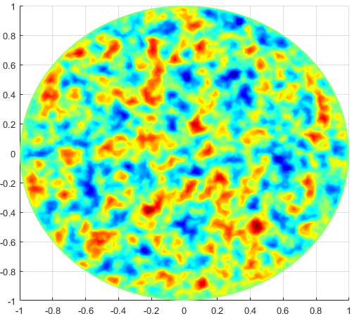 Figure 1
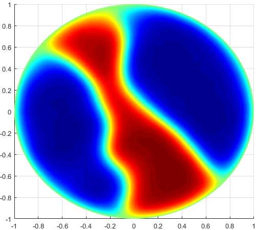 Figure 2
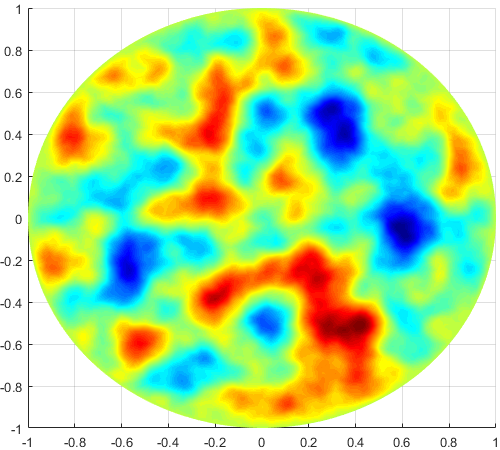 Figure 3
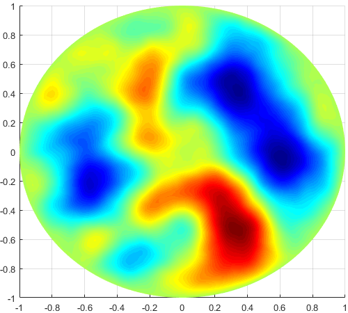 Figure 4
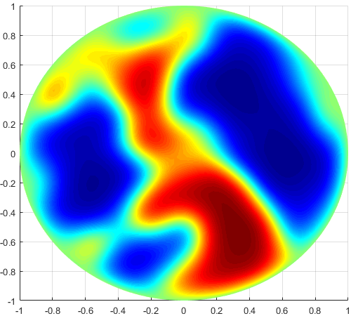 Figure 5
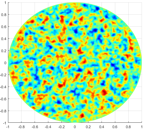 Figure 6
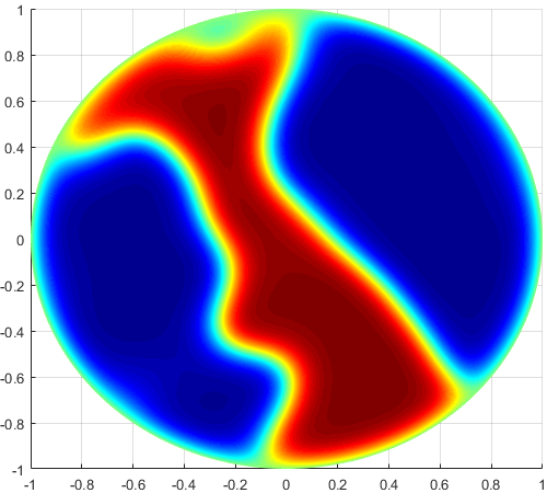 Figure 7
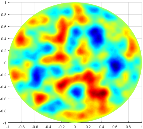 Figure 8
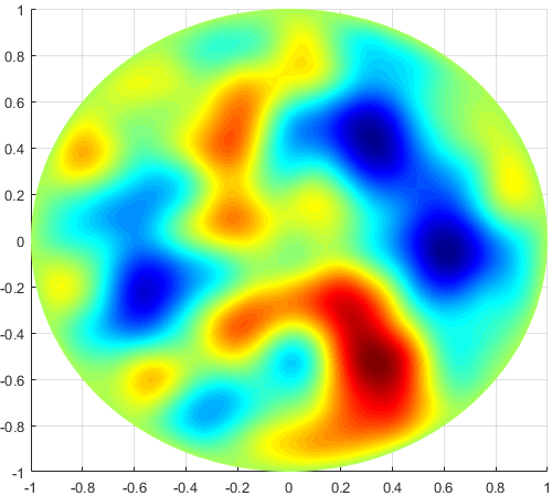 Figure 9
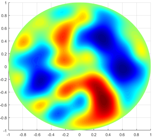 Figure 10
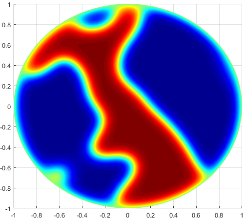 Figure 11
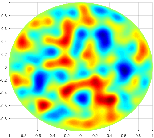 Figure 12
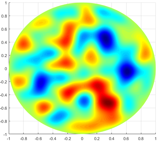 Figure 13
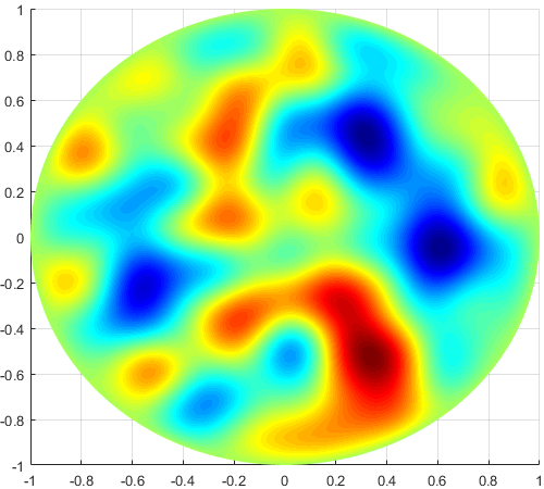 Figure 14
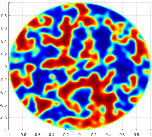 Figure 15
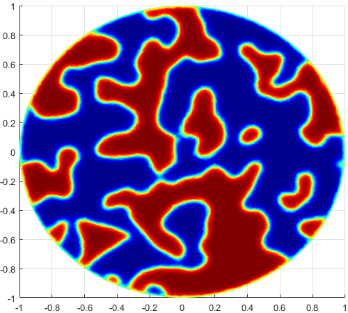 Figure 16
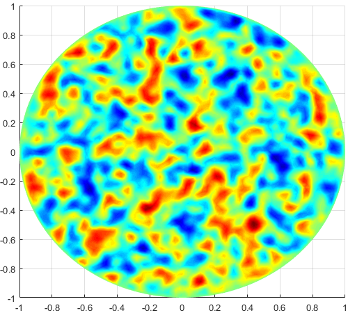 Figure 17
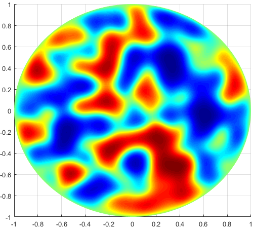 Figure 18
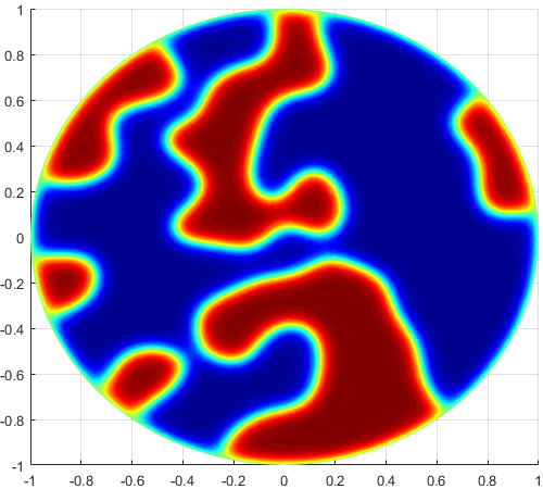 Figure 19
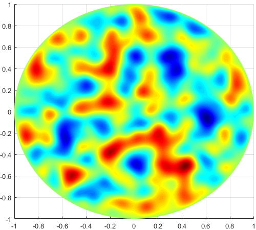 Figure 20
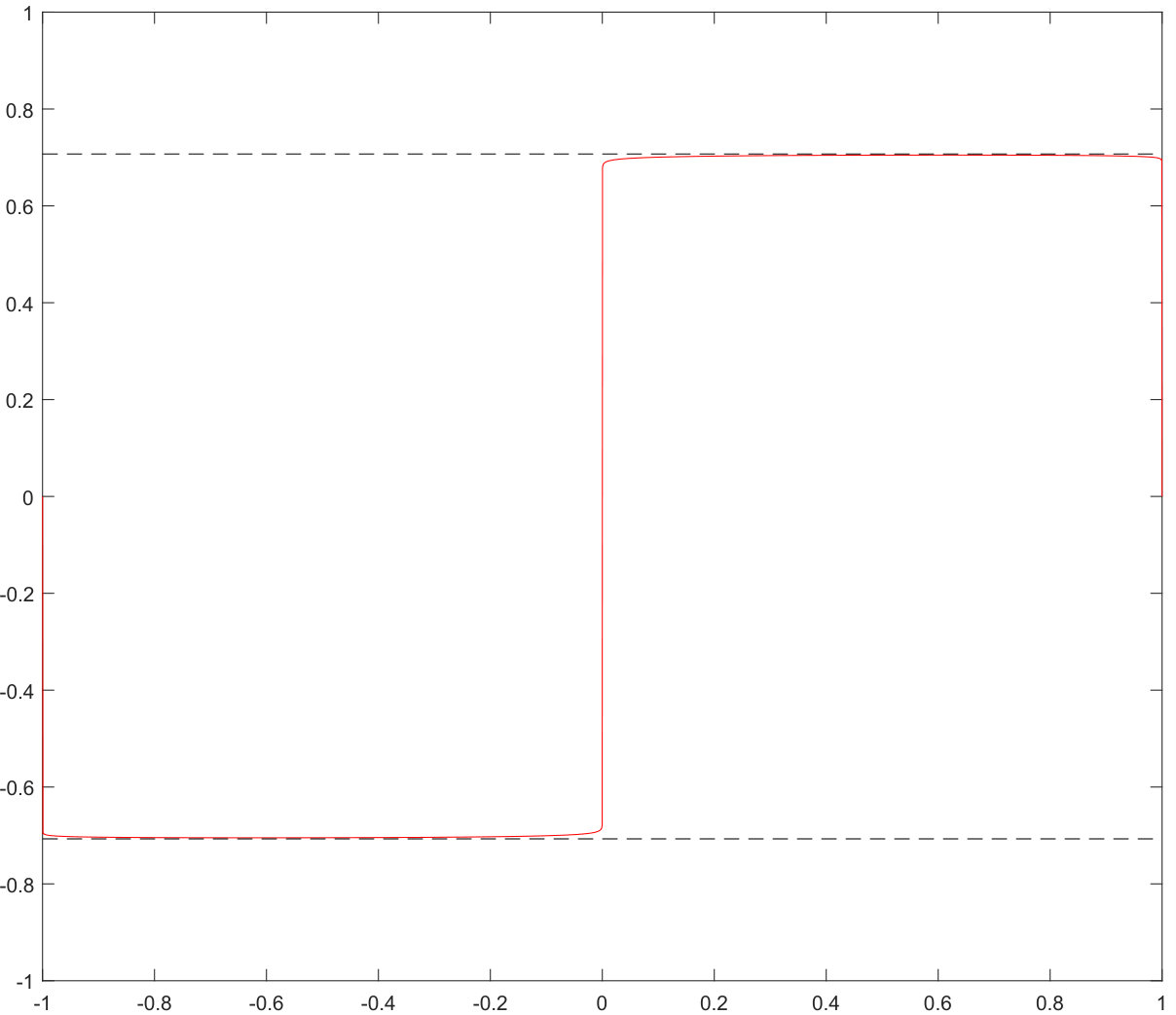 Figure 21
Peer Reviews
No public reviews on file for this paper yet. If you reviewed it on a platform where reviews are public (OpenReview, ICLR, NeurIPS, ICML), you can paste yours below so the community can read it here.
Videos
No videos yet. Explain this paper in a talk, walkthrough, or lecture? Add one.
G. Acosta]http://mate.dm.uba.ar/ gacosta/
Numerical approximations for a fully fractional Allen-Cahn equation
Gabriel Acosta and Francisco M. Bersetche
IMAS - CONICET and Departamento de Matemática, FCEyN - Universidad de Buenos Aires, Ciudad Universitaria, Pabellón I (1428) Buenos Aires, Argentina.
[email protected] [ [email protected]
Abstract.
A finite element scheme for an entirely fractional Allen-Cahn equation with non-smooth initial data is introduced and analyzed. In the proposed nonlocal model, the Caputo fractional in-time derivative and the fractional Laplacian replace the standard local operators. Piecewise linear finite elements and convolution quadratures are the basic tools involved in the presented numerical method. Error analysis and implementation issues are addressed together with the needed results of regularity for the continuous model. Also, the asymptotic behavior of solutions, for a vanishing fractional parameter and usual derivative in time, is discussed within the framework of the -convergence theory.
Key words and phrases:
Fractional Laplacian, Caputo Derivative, Semilinear Evolution Problems
2010 Mathematics Subject Classification:
65R20, 65M60, 35R11
1. Introduction
Several physical and social phenomena have shown to be efficiently described by means of nonlocal models. From anomalous diffusion to peridynamics and from image processing to finance, a rich collection of applications pervades the recent scientific literature, showing the relevance and versatility of this kind of models. In particular, many classical problems have been extended from the local to the nonlocal context in order to capture behaviors that are beyond the modeling capabilities of differential operators. A fact that, in turn, have nurtured the interest in their mathematical foundations as well the corresponding development of numerical methods. Basic examples of this kind of models can be elaborated by considering the fractional Laplace operator,
[TABLE]
where and is a normalization constant. From the probabilistic point of view, corresponds with the infinitesimal generator of a stable Lévy process and can be shown, by means of the Fourier transform [15], that the standard laplacian and the identity operator can be recovered when or , respectively. Thanks to this, the fractional laplacian can be used to model a wide range of anomalous diffusion processes, where particles are allowed to perform arbitrarily long jumps.
On the other hand, even though (1.1) makes perfect sense for , lateral versions are necessary for dealing with the time variable. In such a case, the so-called Caputo and Riemman-Liouville derivatives of order , given respectively by
[TABLE]
and
[TABLE]
are widely used in applications.
Our aim, in this paper, is to extended the classical Allen-Cahn equation
[TABLE]
where and is a domain with smooth enough boundary, to the nonlocal setting. Originally introduced to model the motion of phase boundaries in crystalline solids [8], the unknown function represents the density of the components, describing full concentration of one of them where (or ). Remarkably, the original formulation of the phase-field models [13] contemplates nonlocal interactions, and have been subsequently simplified and approximated by local models.
In this way, we focus on the following problem,
[TABLE]
where belongs to a suitable fractional Sobolev space. Our model (1.4) is based on the Caputo’s version, due to its compliance with standard formulations based on initial conditions [16].
Several numerical techniques have been recently developed for space and time non-local versions of equation (1.3), most of them based on finite differences or spectral methods [7, 21, 22, 27, 28, 35]. Also, numerical methods have been studied for nonlocal versions of related phase separation models, like the Cahn-Hilliard equation [5, 6]. In [19], a rigorous analysis of a general form of problem (1.4) is presented, providing existence and regularity results for a large class of operators, including the fractional Laplacian (1.1) considered here. A similar analysis is also presented in [14].
The article has been organized in the following way. In Section 2, a theoretical treatment of a modified version of problem (1.4) with non-smooth initial datum, including existence, uniqueness and regularity results, is presented. We focus on certain specific kind of regularity results that are tailored to suit the analysis of our numerical method. In Section 3 the numerical scheme, based on Finite Elements for the spatial discretization and convolution quadrature rules for the time variable is presented and the error estimation is treated in Section 4 . Some arguments, developed in Section 5, show that our analysis can be extended to the model problem (1.4). A complementary result, inspired by the behavior of solutions obtained in our numerical simulations, is given in Section 6 where we study the asymptotic behavior of solutions of (1.4), with , when the fractional parameter . Strange behaviors, as the displacement of the equilibrium states, are analyzed by means of the Gamma-convergence theory applied to the associated non-local Ginzburg-Landau energy functional. Finally, numerical experiments are shown in Section 7.
2. A Fractional Semilinear Equation
In order to study (1.4), we temporally focus first on a ”restricted” problem,
[TABLE]
where verifies the following conditions (H1) and (H2),
[TABLE]
[TABLE]
Clearly, the function of problem (1.4) does not comply with (H2). The goal is to apply later our results to a problem of the form (2.1) with a source term that, in addition to and , agrees with in some interval , for an arbitrary . In this case, the condition implies which in turn allows to remove (H2) in this context. Therefore, for such initial condition, (2.1) and (1.4) are equivalents. This bound is obtained indirectly through the analysis of the semi-discrete in time scheme deferred to Section 5.1.
2.1. Weak formulation
For any , we consider an open set . We define the fractional Sobolev space as
[TABLE]
This set, together with the norm becomes a Hilbert space.
Another important space of interest for the problem under consideration is that of functions in supported inside ,
[TABLE]
The bilinear form
[TABLE]
constitutes an inner product on . The norm induced by the bilinear form, which is just a multiple of the -seminorm, is equivalent to the full -norm on this space, due to the fact that a Poincaré-type inequality holds in it. See, for example, [3] for details.
We call a weak solution of (2.1), if and
[TABLE]
almost everywhere in .
Let us note that, defining the operator ,
[TABLE]
the first identity of (2.5) can be rewritten as
[TABLE]
a.e. in .
2.2. Solution representation
For the fractional eigenvalue problem,
[TABLE]
it is well-known that there exists a family of eigenpairs , such that
[TABLE]
with the eigenfunctions’s set constituting an orthonormal basis of .
Remark 2.1*.*
Unlike eigenfunctions of the classical laplacian, solutions of (2.8) are in general non-smooth. Indeed, considering a smooth function that behaves like near to , all eigenfunctions belong to the space (the is active only if ) and does not vanish near [20, 33]. Moreover, the best Sobolev regularity guaranteed for solutions of (2.8) is for (see [10]).
With , solutions of (2.8), and the Mittag-Leffler functions , given by
[TABLE]
for each and , we define the operators
[TABLE]
and
[TABLE]
for every . Following the theory for the linear case (see for instance [2]), the solution of (2.1) should, at least formally, satisfy the integral equation
[TABLE]
We say that is a mild solution of problem (1.4), if is a solution of equation (2.12) and in this case, we use the notation .
For technical purposes we define the interpolated norm
[TABLE]
It can be easily verified that , , and . Additionally, we denote , , the space induced by the norm (2.13).
The following two lemmas provide helpful estimates for the operators (2.10) and (2.11).
Lemma 2.2**.**
Consider , then we have
[TABLE]
Proof.
The proof is analogous of that of [23, Lemma 2.2] (see also [9, Lemma 2.0.2]). ∎
Lemma 2.3**.**
If , , then for
[TABLE]
Proof.
The proof can be carried out as in [24, Theorem A.2] (see also [9, Lemma 2.0.3]). ∎
2.3. Existence and Uniqueness
For the sake of simplicity we are going to consider along this section.
To obtain an existence and uniqueness result for the integral equation (2.12), we use standard fixed point arguments adapted to the present context. Our approach follows [14] and [26]. For and , we introduce the space,
[TABLE]
where is defined as
[TABLE]
The inclusion , for , follows immediately from the definition, while the fact that is a Banach space can be proved by means of standard arguments. In the sequel, the parameter plays a role in connection with the regularity of the initial datum . In particular, if for some positive , we show below that . This condition on is important for the analytical treatment of the numerical error and a fundamental assumption for a right definition of the Caputo operator (1.2).
Remark 2.4*.*
It is important to observe that we necessarily need for some positive . Otherwise, the fractional derivative in time could not be well defined for solutions of problem (1.4). In fact, even considering a simpler problem, taking in (1.4), it is possible to construct a function in such a way that for all and, for that initial datum, the solution . We refer to [9, Remark 2.1.5] for details.
The following is a local existence result.
Theorem 2.5**.**
Suppose that for some and . Then, there exist small enough, such that equation (2.12) has a unique solution .
Proof.
First, we define the operator
[TABLE]
and . It can be easily verified that is a closed set. Our goal is to show that there are parameters and , in such a way that we can apply Banach’s fixed point theorem. That is, we look for and , such that maps into itself, and results in a contraction over .
Indeed, observing first that for all , then the condition is satisfied for every output of . Furthermore, by means of Lemma A.1, it can be seen that . Suppose now , from (2.16), Lemma 2.2 and the definition of , we have
[TABLE]
[TABLE]
[TABLE]
using the boundedness of and computing the resulting integral, together with the fact , we get
[TABLE]
With the same idea we can obtain
[TABLE]
On the other hand, by means of Lemma A.1, we have
[TABLE]
[TABLE]
and we can write
[TABLE]
[TABLE]
[TABLE]
where we have applied Lemma 2.3, Lemma 2.2, the fact that and . The integral in the second term can be estimated in terms of the beta function . Indeed, making the change of variables , we obtain
[TABLE]
[TABLE]
Combining (2.17), (2.18) and (2.20), we have
[TABLE]
where . Then, fixing , we can choose small enough to satisfy the inequality . Hence, for this , maps into itself.
Now we want to see that is a contraction over . Indeed, let and , using and Lemma 2.2, we have
[TABLE]
[TABLE]
[TABLE]
[TABLE]
[TABLE]
With similar arguments it can be seen that
[TABLE]
Recalling the equality (2.19), we have that
[TABLE]
[TABLE]
Using the identity
[TABLE]
and the fact that , , , , we can write
[TABLE]
[TABLE]
[TABLE]
[TABLE]
[TABLE]
where the integrals in the last inequality have been estimated in terms of the beta function, as in (2.20), and .
Finally, combining (2.21), (2.22) and (2.23), we can conclude that
[TABLE]
with , and it is clear that we can choose small enough, such that results in a contraction over . Hence, for that , a unique solution for problem (1.4) in the interval . ∎
Now we need to derive an a priori estimate for the time derivative of the solution. To this end, we first recall the following Gronwall type inequality .
Lemma 2.6**.**
Let the function be continuous for . Then, if
[TABLE]
for some constants , and , there exists a constant such that
[TABLE]
Proof.
See, for instance, [17] Lemma 6.3. ∎
Now, we are ready to state the following result.
Lemma 2.7**.**
Let with and , there exists a constant such that
[TABLE]
Proof.
For we can write
[TABLE]
[TABLE]
[TABLE]
[TABLE]
[TABLE]
[TABLE]
[TABLE]
Now, considering small enough, and taking norms at both sides of the equality; using Lemma 2.3 in the first term on the left side; estimation (2.15), and estimation in the second term and the same idea in the last one, we obtain
[TABLE]
[TABLE]
[TABLE]
Finally, applying Lemma 2.6 we derive (2.25).
∎
Combining the former results, we are now able to prove the global existence of the solution.
Theorem 2.8**.**
Under the hypotheses of Theorem 2.5, let be the solution of (2.16) defined in and consider fixed numbers and , such that . Then, there exists a constant such that if , can be extended to as a solution of (2.16).
Proof.
We are going to consider the space , for some , and , defined as , where is the solution of (2.16) over . Observe that, with this definition, is a closed subset of . Our goal is, as in the proof of Theorem 2.5, to apply Banach’s fixed point Theorem, showing that there exist and , such that is a contraction over , and maps into itself.
Suppose , proceeding similarly as in (2.17), using the boundedness of , we can obtain
[TABLE]
[TABLE]
With the same idea we obtain
[TABLE]
Also, applying the same arguments used to arrive to (2.20), along with the fact that for all together with the fact that , we get
[TABLE]
[TABLE]
[TABLE]
[TABLE]
[TABLE]
[TABLE]
where in the last inequality we have used (2.25). Now, making the change of variables , we have
[TABLE]
[TABLE]
and
[TABLE]
[TABLE]
where we have estimated using the fact that .
Applying this estimation to (2.30), we obtain
[TABLE]
and combining (2.31) with (2.28) and (2.29), we obtain
[TABLE]
If we choose , taking we have .
Finally, we only need to show that is a contraction on . Consider and , proceeding as in (2.21), and taking advantage of the fact that for all , we can estimate
[TABLE]
[TABLE]
[TABLE]
[TABLE]
[TABLE]
where in the last step we use the bound , with .
Also, arguing as in (2.23), we have
[TABLE]
[TABLE]
[TABLE]
[TABLE]
[TABLE]
with the same arguments used to bound we arrive to
[TABLE]
Then, we can assert that and we can choose such that results in a contraction. Since depends on and , the statement of the theorem follows.∎
Notice, in previous Theorem, that does not depend on . As a consequence, we have proved that equation 2.12 has a unique solution in . Moreover, in view of the regularity of functions belonging to the space , we can assert that a mild solution is also a weak solution.
3. Numerical Scheme
3.1. Semi-discrete Scheme
Let be a shape regular and quasi-uniform admissible triangulation of . With we denote the continuous piecewise linear finite element space associated with , that is,
[TABLE]
Then, semi-discrete problem formulation reads: find such that
[TABLE]
Here, , and denotes the projection on . Also, defining the discrete fractional Laplacian as the unique operator that satisfies we may rewrite (3.1) as
[TABLE]
We also define the discrete versions of and . In order to do this, consider an orthonormal basis of , and define
[TABLE]
and
[TABLE]
3.2. Discretizing the Caputo derivative
In order to set a fully discrete scheme, we need to discretize the Caputo operator. This can be done by means of the well known relation between the Caputo derivative , and the Riemann-Liouville operator , that reads
[TABLE]
for (see, for instance, [16] Theorem 3.1) that holds for a smooth enough function . Applying (3.5) to problem (3.2), we can reformulate it in terms of the Riemann-Liouville operator as follow,
[TABLE]
The advantage here is that the R-L derivative can be approximated by means of a convolution quadrature rule. That is, dividing the interval uniformly with time step , and letting , a discrete estimation of can be defined as
[TABLE]
Here, the weights are obtained as the coefficients of the power series expansion \Big{(}\frac{1-\xi}{\tau}\Big{)}^{\alpha}=\sum^{\infty}_{j=0}\omega_{j}\xi^{j}. Fast Fourier Transform can be used for an efficient computation of , (see [32] Section 7.5). Alternatively, a useful recursive expression is also given in [32],
[TABLE]
It is not our intention to give an exhaustive description of this method and we refer the reader to [2, 24] (see also [29, 30] for further details). An advantage of convolution quadratures is that error estimates can be delivered without the assumption of excessively restrictive regularity properties on the solution. This is a fact of paramount importance as one can learn from [36].
The following result (Theorem 5.2, [29]) will play a central role in the error estimation below.
Lemma 3.1**.**
Let be a complex valued or operator valued function which is analytic in a sector , with , and bounded by for some . Then for , the operator satisfies
[TABLE]
Finally, another useful property of the operator is the associativity. That is, let be operators as in Lemma 3.1, and an analytic function, we have
[TABLE]
3.3. Fully discrete scheme
Replacing the Riemann-Liouville derivative by its discrete version given by (3.7), we can formulate the fully discrete problem as: find , with , such that
[TABLE]
For the sake of the reader’s convenience, we include a vectorial form of the fully discrete scheme. Let be the Lagrange nodal basis that generates . Let , be such that , where denotes the solution of the fully discrete problem. Then, we may formulate (3.10) in the following vectorial non-linear equation:
[TABLE]
Where and are the mass and stiffness matrices respectively. That is, and .
The computation and assembly of the stiffness matrix in dimension greater than one is not a trivial task. Nevertheless, this problem for two-dimensional domains is treated in [1], where the authors provide a short MATLAB implementation to this end. Also we can mention [4, 25] where some clever ways to reduce the complexity of the assembling process are analyzed.
Since (3.10) is not a linear equation, it is not clear a priori that there exist a solution. In that way, next result gives us existence and uniqueness for problem (3.10).
Theorem 3.2**.**
There exist small enough, such that problem (3.10) has a unique solution for all .
Proof.
Recalling that , dividing equation (3.10) by on both sides, we obtain
[TABLE]
Observe that, since for all , it is true that
[TABLE]
for all . Now, suppose by induction, that we have a solution for all , and define as
[TABLE]
Applying a fixed point argument, if is a contraction over , then problem (3.10) will have a unique solution. To this end, suppose that we have and . Then, using we have
[TABLE]
[TABLE]
Taking , we have that is a contraction, and problem (3.10) has a unique solution. ∎
4. Error estimation
For the sake of simplicity we are going to consider through this section.
4.1. Error estimates for the semidiscrete scheme
For the following linear problem
[TABLE]
where and the corresponding semi-discrete approximation
[TABLE]
with , we have the following two results [2].
Theorem 4.1**.**
Let and be solutions of (4.1) and (4.2) respectively with , , and right hand side . Then it holds,
[TABLE]
where and , with arbitrary small.
Theorem 4.2**.**
Let and be as in Theorem 4.1 with and initial datum equal to zero. Then, there exists a positive constant such that
[TABLE]
with as in Theorem 4.1.
From this, we can estimate the error for the semi-discrete scheme (3.1).
Theorem 4.3**.**
Let and be the the exact and the semi-discrete solution of (2.5) and (3.1) respectively. And let with and with . Then there exist a positive constant such that
[TABLE]
With as in Theorem 4.1.
Proof.
We can write the solution and its semi-discrete approximation as and respectively. Then, defining , we have
[TABLE]
[TABLE]
Using Theorem 4.1 in the first term; , and (2.15) in the second term; Theorem 4.2 with and in the last term, we have
[TABLE]
Then, applying Lemma 2.6 we derive (4.3). ∎
4.2. Error estimation for the fully discrete scheme
Consider the discrete problem of find , , such that
[TABLE]
with , for all . Recalling that , and defining , we can rewrite (4.4) as
[TABLE]
If we define as the coefficients of the series expansion of , from the definition of we have for all . And we can write as a function of in a recursive expression
[TABLE]
with recursively defined as
[TABLE]
As we have observed in the proof of Theorem 3.2, we have
[TABLE]
Then, from (4.7), and recalling that for , we have
[TABLE]
Defining the sequence
[TABLE]
it is possible to check that
[TABLE]
In order to bound the error, it will be useful to know about the asymptotic behavior of . This is analyzed in the next lemma proved in Appendix A.
Lemma 4.4**.**
Let be the coefficients of the power series expansion of , with , and the sequence recursively defined in (4.9). Then, .
Theorem 4.5**.**
Let and be the solution of (1.4) and (3.10) respectively Consider for some and with . Then, if , for a sufficiently small there exist a positive constant such that
[TABLE]
[TABLE]
With as in Theorem 4.1.
Proof.
In view of Theorem 4.3, we only need to estimate , with the semi-discrete solution. Considering the sector , it can be seen that the function is analytic in with . Then, from the semi-discrete and fully discrete scheme, we have
[TABLE]
and
[TABLE]
Subtracting both expressions we obtain an equation for ,
[TABLE]
[TABLE]
[TABLE]
The norm of the first term can be estimated arguing as in [2, Theorem 5.3] (see also [9, Theorem 4.2.8]). Since we obtain
[TABLE]
with . For the second term, using property (3.9), we can split as follow
[TABLE]
[TABLE]
[TABLE]
Using Lemma 3.1 with , along with the fact that , we can estimate
[TABLE]
On the other hand, noticing that Lemma 2.7 can be easily extended to , in order to get ; using again Lemma 3.1, the fact that , and writing , we have
[TABLE]
[TABLE]
[TABLE]
where in the last inequality we have estimated the integral in terms of the beta function , as in Theorem 2.5.
Now, we observe that the last term is a solution for (4.4), with . Then, in view of (4.6) and (4.10), and using again that , we have
[TABLE]
where is the sequence defined in (4.9).
Using that with , and the fact that (given by Lemma 4.4), we can derive the following
[TABLE]
[TABLE]
Taking in such a way that and , we can subtract the last term on the right from both sides an obtain
[TABLE]
Finally, applying Lemma A.2 (a discrete analog of Lemma 2.6), we have
[TABLE]
for some .
From this, (4.13), and (4.3), we can derive (4.11). ∎
5. Analysis of the fractional Allen-Cahn equation
5.1. bounds
At this point we need to recall some results that play an important role in our analysis. The following two theorems summarize classical global and interior regularity of solutions for the following problem,
[TABLE]
We refer to [18] for further details about (5.1).
Theorem 5.1**.**
Let be any bounded domain, , and be the solution of (5.1). If ; then . Moreover, where the constant depends only on and .
Theorem 5.2**.**
Let be a bounded domain of , and let be a solution for (5.1). If , for each define . Then, if is not an integer, for every we have
[TABLE]
with .
We devote the remaining sections to problem (1.4). In order to exploit the results obtained for (2.1) we need to work with a truncated version of . In this way, along this section we assume that our source term verifies (2.2), (2.3) and agrees with in an interval , for some . In order to prove that, in this case, the solution remains bounded between and for any such that , we are going to define first a discrete in time problem. That is, find , with , such that
[TABLE]
The proof of the existence and uniqueness of solutions for this problem is similar to the one given for the fully discrete case. For the solution of this problem, we have the following result.
Theorem 5.3**.**
Consider the semi-discrete in time scheme (5.3) with , then there exist in such a way that if (5.3) has a solution , , with for all . Moreover if for all , then for all and .
Proof.
Suppose we have a solution with the desire properties for all . From (5.3) we have the identity
[TABLE]
where .
First we want to show that there exists that satisfies equation 5.4. In order to do that, we define the map
[TABLE]
We want to verify that is a contraction in . From the fact that is a maximal monotone operator (see [12]), we know that . Let and , we can estimate
[TABLE]
[TABLE]
Then, for a small we have that is a contraction. Hence, there exists a unique solution for (5.4), and the identity
[TABLE]
is satisfied. Since the right hand side belongs to , applying the Theorem 5.1, we can conclude that for all .
Now, we want to see that if the initial data is regular enough, then the solution remains bounded between and . Indeed, suppose we have and for all , for all . If we take a fixed with in Theorem 5.2, and use the the fact that , then and we can conclude that . A repeated application of this argument, along with the fact that , implies that for some only depending on . Since can be arbitrary small, we can assert that , and then, .
On the other hand, the semi-discrete in time scheme gives us the relation
[TABLE]
which can be rewritten as
[TABLE]
with . Suppose that there exist some such that achieves its maximum on that point, and . Recall that for all . From the regularity of , it can be shown that (see [18, Lemma 3.9]). Then, from the fact that , we have , which implies
[TABLE]
Observing the fact that is a positive and strictly decreasing sequence, it is possible to show that there exist , such that (see [9, Lemma 5.2.4]), and then . The contradiction came from the assumption that .
Now we want to see that the same bound holds for less regular initial data. To this end, applying a density argument, suppose is a solution for (5.3) with , . Consider , with for all , and in .
Let be the solution of (5.3) with initial data . Calling , we have the equation
[TABLE]
and taking norms we obtain
[TABLE]
Choosing such that , recalling that , and applying a discrete Gronwall type inequality we have
[TABLE]
with , and then, with .
Since , then for all , and for all . Hence, for a fixed , we can construct a sub-sequence , such that a.e. , and conclude that . ∎
Finally, proceeding analogously as in Theorem 4.5, we can derive the following error estimation.
Theorem 5.4**.**
Let and be the solution of (1.4) and (5.3) respectively, with , with . Then, if , for a sufficiently small exists a positive constant such that
[TABLE]
Now, consider . Given a fixed we can construct a family of nested partitions of [0,T] with , , and if , in such a way that belongs to all the partitions. Let be the solution of (5.3), and the solution of (2.5), using Theorem 5.4 we have that in . So, we can extract a subsequence such that a.e. . Using 5.3, we know that , and then, . We can summarize this observation in the following result.
Theorem 5.5**.**
Let a solution of (2.7) with . Then for all .
This theorem implies that all the analysis displayed up to here remains valid replacing by and therefore to the Allen-Cahn equation (1.4).
6. Discussion about the asymptotic behavior with
Considering now the usual derivative in time (), the Allen-Cahn equation can be understood as a gradient flow in , minimizing the free energy functional
[TABLE]
with (see for example [5]). It is well known that the size of affects the interface width of the minimizers of . That is, interface width tends to zero with . This fact can be easily derived from expression (6.1), observing that the right term, which penalizes the variation of , tends to lose relevance as goes to zero, forcing the minimizer to take values into the set of minimizers of , that is values belonging to . However, since , the right term promote the minimization of the interface length (for ), which implies that the limit behavior cannot be understood as the minimization of with . In [34], Savin and Valdinoci show, by means of -convergence theory, that the limit behavior of the problem of minimizing tends to a minimal surface problem if , and to a non-local version of the minimal surface problem for .
In our case, numerical experiments (see Figure 2) show that the interface width tends to become thinner when the parameter goes to zero, suggesting that (as in the case ) a minimizer of should approximate a binary function when . This behavior was also observed in [6], where authors derive the scaling law , with denoting the interface width. On the other hand, a displacement of the equilibrium states have been observed in our numerical experiments for small values of the fractional parameter (see Figure 1).
Motivated by the previous observation, the aim of this section is to analyze the asymptotic behavior of the minimizers of with tending to zero. To this end, we are going to follow the ideas displayed in [34], and study the -convergence of a suitable modification of the functional . By means of this framework, it is possible to conclude that the minimizers of (6.1) approach binary functions, and the equilibrium states should be placed near and for small values of the fractional parameter .
6.1. -convergence when .
Since -convergence may not be a usual concept in numerical analysis, we start this section by giving its definition and basic properties, and we refer to [11] for further details.
Let be a topological space, and , , a sequence of functionals. Then, we say that -converge to , if the following conditions holds:
- •
For every sequence such that , then
[TABLE]
- •
For every , there exist a sequence converging to such that
[TABLE]
Also, we define a complementary concept. We say that the family has the equi-coerciveness property if for all exists a compact set in such a way that for all .
These two concept allow us to say something about the limiting behavior of the minimizers of in terms of the minimizers of . That is, if is a minimizer of , then every cluster point of (if exist) is a minimizer of . This can be summarized as follow
[TABLE]
In order to study the -convergence of , we must set an appropriate domain for ,
[TABLE]
And we are going to consider this space furnished with the norm . Note that if but , then we can define .
From the definition of , and supposing , we have
[TABLE]
[TABLE]
and, denoting as the Fourier transform of , we know from [15] and Plancharel’s identity that and Then we have
[TABLE]
so we can rewrite as
[TABLE]
with .
Since we have , is a double-well type potential with minimizers .
Noticing that , we define a new auxiliary functional
[TABLE]
and, for the sake of simplicity, we redefine as so now . Fixing and , it is easy to check that is a minimizer of if and only if is a minimizer of . So we focus our study on the asymptotic behavior of .
Defining the functional
[TABLE]
with , we have the following theorem.
Theorem 6.1**.**
Let and defined as before, then .
Proof.
Let with in , and suppose w.l.o.g, that takes values in a discrete set. First, we want to see
[TABLE]
Indeed, suppose that , in other case there is nothing to prove. If we choose a suitable sub-sequence of such that a.e. and , then
[TABLE]
We first analyze the left term of the right hand side of (6.4). In this case we have
[TABLE]
[TABLE]
From the fact that in norm, we have point-wise, and we also have . Then, using Fatou’s Lemma, we get the estimation
[TABLE]
On the other hand, since , we can estimate the second term as follow
[TABLE]
[TABLE]
where in the last inequality we have use the reverse Fatous’s Lemma.
Hence, the first term on the right hand side of (6.4) must be a finite number. This implies that and thus, with .
Since we have chosen in such a way that a.e., we have that a.e., then must have the form Now, we can estimate
[TABLE]
[TABLE]
and (6.3) follow.
Finally we only need the to verify that if , then
[TABLE]
To this end, suppose , otherwise there is nothing to prove. In this case we have The fact that with , implies that is decreasing in . Then
[TABLE]
[TABLE]
Then, using Monotone Convergence Theorem on the integral over , and Dominated Convergence Theorem over , we have which proves (6.6).
∎
6.2. Equi-coerciveness of
To complete the analysis we prove the equi-coerciveness of .
Theorem 6.2**.**
Suppose , and , such that for all . Then there exist and a subsequence , such that in .
Proof.
First we observe that, as before, we have
[TABLE]
Since and for all , we can assert that
[TABLE]
The fact that , implies for all , and then
[TABLE]
Now we want to show that (6.7) implies that functions in the set keep a substantial part of their mass uniformly bounded. Namely, given , there exist such that
[TABLE]
By contradiction suppose that there exist such that for every there is a number , in such a way that
[TABLE]
Choosing such that , with the constant in (6.7), and the one in (6.8) , we have
[TABLE]
[TABLE]
which, in view of (6.7) results in a contradiction. Hence, assertion (6.9) holds.
On the other hand, the fact that , implies that this sequence is uniformly bounded in , and then, we can extract a weakly convergent subsequence . Let such that , our goal now is to show that strongly in , which implies strong convergence in since .
To this end, we only need to verify that or, equivalently, . From (6.9), and the fact that , we can take large enough, in such a way that and Then we have
[TABLE]
[TABLE]
Since is supported in , for all , weak convergence implies for all . And, as we have observed before, since for all , for all . Hence, we can apply Dominated Convergence Theorem in (6.10) and say that there exists in such a way that if then
[TABLE]
Since can be arbitrary small, we have , and the statement of the theorem follows.
∎
7. Numerical experiments
In this section, three numerical examples are presented in order to explore the behavior of the solution under fractional parameters and .
For the first example, we have used , a uniform mesh consisting of nodes, , , , and the function as initial data. Here, the aim is to obtain some experimental support for the ideas displayed in section 6, that is, the behavior with a small parameter . Numerical results are summarized in Figure 1, and equilibrium values far from and can be observed. Furthermore, equilibrium values seem to be placed near the values predicted in section 6 or, in other words, the solution seems to approximate a minimizer of (6.2).
Example 2 and 3 (spinodal decomposition) are shown in Figure 2 and 3 respectively. Here we have used as the unitary ball, a uniform triangulation consisting of triangles, , and random noise as initial data. In example 2 (Figure 2), the parameter is fixed in , and results for several values of are shown. Can be observed the fact that, as we have mentioned in section 6, the smaller the parameter , the thinner the interface. Finally, example 3 (Figure 3) shows the behavior for fractional values of the parameter , with .
Appendix A Auxiliary results
Lemma A.1**.**
Let , with differentiable in in such a way that with for all . Then we have
[TABLE]
Proof.
We write
[TABLE]
[TABLE]
From the mean value inequality in Banach spaces (see, for instance, [31, Appendix B]) we can estimate
[TABLE]
[TABLE]
This, along with the fact that exists in , allows us to use the Domitated Convergence Theorem (see [31, Appendix B]) and get
[TABLE]
On the other hand, from the fact that is a continuous function in , we have
[TABLE]
where the convergence is in sense.
Finally, combining (A.2), (A.3) and (A.4), we obtain (A.1).
∎
Lemma A.2**.**
For consider with and . If
[TABLE]
for all , with some constants , , and , , then there exist a constant such that
[TABLE]
Proof.
First, we observe the following relation. For , we have
[TABLE]
[TABLE]
where denotes the beta function.
Now, if we choose the smallest such that and iterate (A.5) times, using relation (A.6) we obtain
[TABLE]
with and . If we can derive (A.6) by means of a standard discrete Gronwall type inequality. Otherwise, we take and using (A.8) we obtain
[TABLE]
and deduce , again by means of a standard Gronwall type inequality.
∎
Proof.
(of Lemma 4.4) From the definition of , we know that Then, defining , and recalling that , we have Now, defining , from the definition of , and using the Cauchy product for power series, the following equality can be easily checked,
[TABLE]
Recalling that , and , from (A.9) we can obtain an explicit expression for , It is well known that series expansion of is Then where
Finally, by means of basic Gamma function properties, we can verify that , and hence, . ∎
Acknowledgments
The authors thank Prof. Julián Fernández Bonder and Prof. Ciprian Gal for their valuable comments which helped to improve the manuscript.
The reference list from the paper itself. Each links out to its DOI / PubMed record.
- 1[1] G. Acosta, F. Bersetche, and J.P. Borthagaray. A short FEM implementation for a 2d homogeneous Dirichlet problem of a fractional Laplacian. Comp. Math. Appl. , 74(4):784–816, 2017.
- 2[2] G. Acosta, F. M. Bersetche, and J. P. Borthagaray. Finite element approximations for fractional evolution problems. Fractional Calculus and Applied Analysis , 22(3):767–794, 2019.
- 3[3] G. Acosta and J. P. Borthagaray. A fractional Laplace equation: Regularity of solutions and finite element approximations. SIAM J. Numer. Anal. , 55(2):472–495, 2017.
- 4[4] M. Ainsworth and C. Glusa. Aspects of an adaptive finite element method for the fractional laplacian: a priori and a posteriori error estimates, efficient implementation and multigrid solver. Computer Methods in Applied Mechanics and Engineering , 327:4–35, 2017.
- 5[5] M. Ainsworth and Z. Mao. Analysis and approximation of a fractional Cahn–Hilliard equation. SIAM Journal on Numerical Analysis , 55(4):1689–1718, 2017.
- 6[6] M. Ainsworth and Z. Mao. Well-posedness of the Cahn–Hilliard equation with fractional free energy and its fourier galerkin approximation. Chaos, Solitons & Fractals , 102:264–273, 2017.
- 7[7] G. Akagi, G. Schimperna, and A. Segatti. Fractional Cahn–Hilliard, Allen–Cahn and porous medium equations. Journal of Differential Equations , 261(6):2935–2985, 2016.
- 8[8] S. M. Allen and J. W. Cahn. A microscopic theory for antiphase boundary motion and its application to antiphase domain coarsening. Acta Metallurgica , 27(6):1085–1095, 1979.