Interacting Langevin Diffusions: Gradient Structure And Ensemble Kalman Sampler
Alfredo Garbuno-Inigo, Franca Hoffmann, Wuchen Li, Andrew M. Stuart

TL;DR
This paper introduces a derivative-free ensemble Kalman sampler based on interacting Langevin diffusions with a novel gradient flow structure, demonstrating its theoretical properties and practical effectiveness in Bayesian inverse problems.
Contribution
It develops a new gradient flow framework for interacting Langevin diffusions and proposes a derivative-free ensemble Kalman sampler with proven convergence properties.
Findings
The invariant measure matches that of a single Langevin diffusion.
Exponential convergence to the invariant measure is demonstrated.
Numerical experiments show the sampler's effectiveness in Bayesian inverse problems.
Abstract
Solving inverse problems without the use of derivatives or adjoints of the forward model is highly desirable in many applications arising in science and engineering. In this paper, we propose a new version of such a methodology, a framework for its analysis, and numerical evidence of the practicality of the method proposed. Our starting point is an ensemble of over-damped Langevin diffusions which interact through a single preconditioner computed as the empirical ensemble covariance. We demonstrate that the nonlinear Fokker-Planck equation arising from the mean-field limit of the associated stochastic differential equation (SDE) has a novel gradient flow structure, built on the Wasserstein metric and the covariance matrix of the noisy flow. Using this structure, we investigate large time properties of the Fokker-Planck equation, showing that its invariant measure coincides with that of…
Click any figure to enlarge with its caption.
 Figure 1
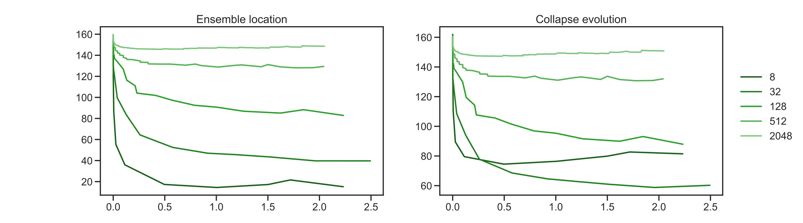 Figure 2
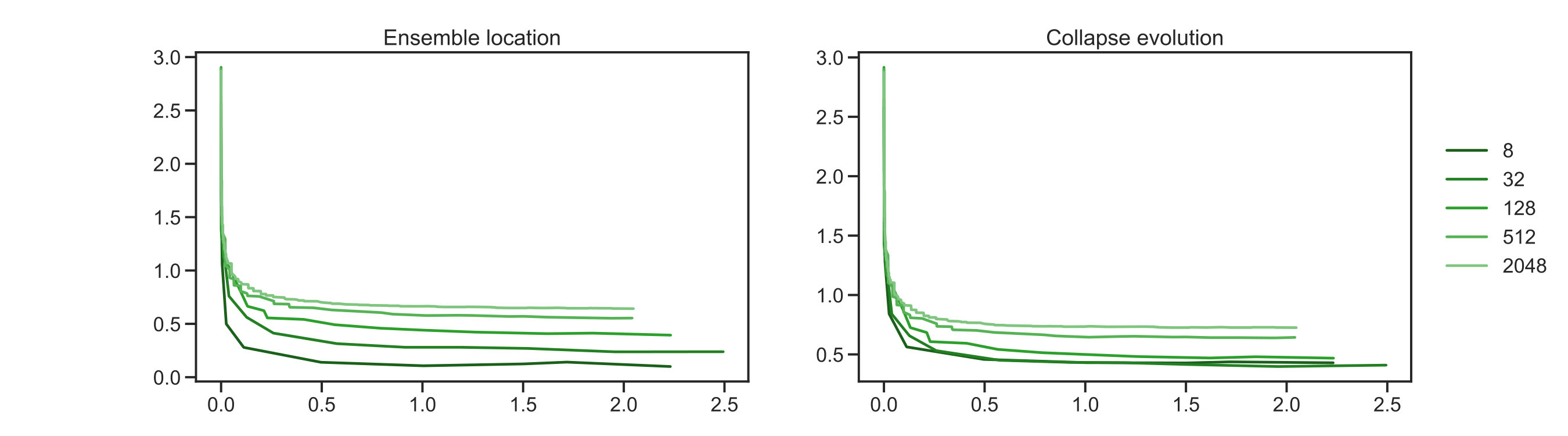 Figure 3
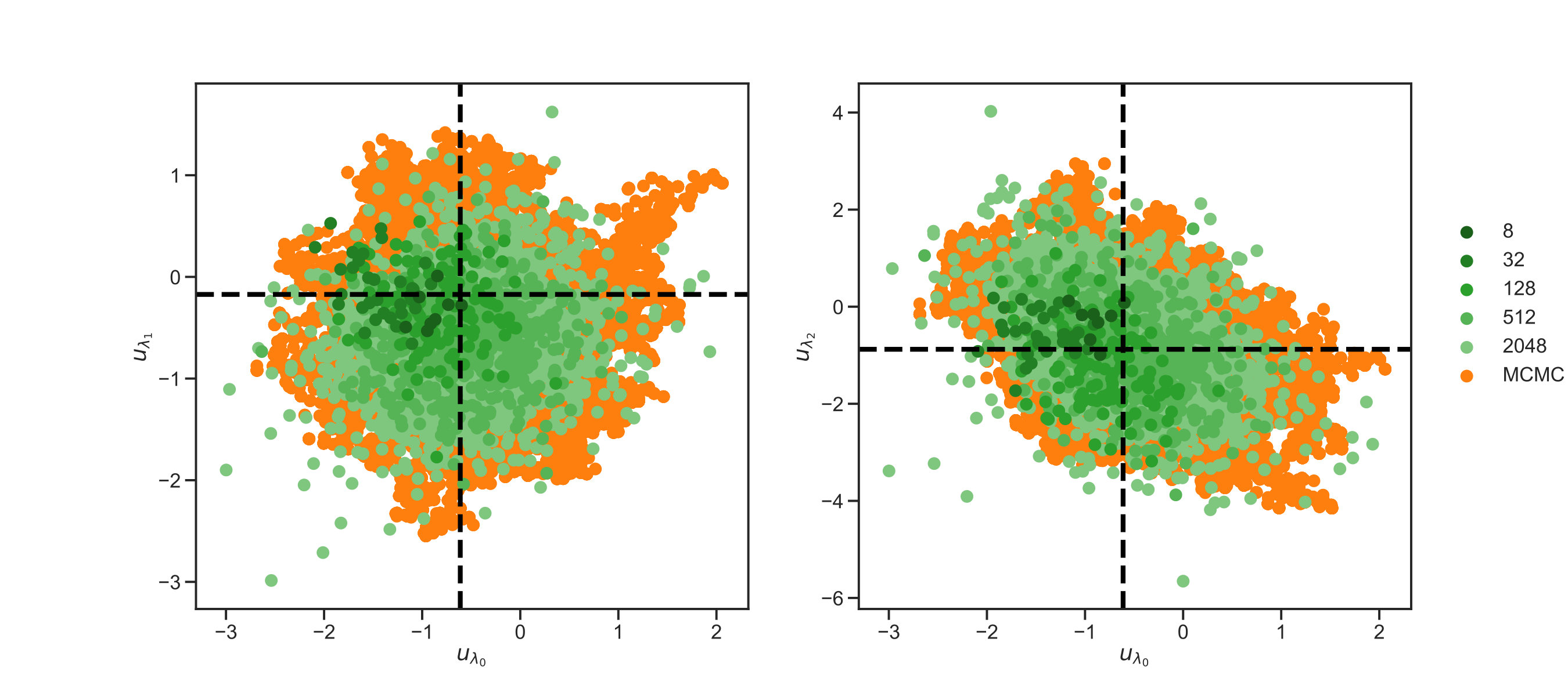 Figure 4
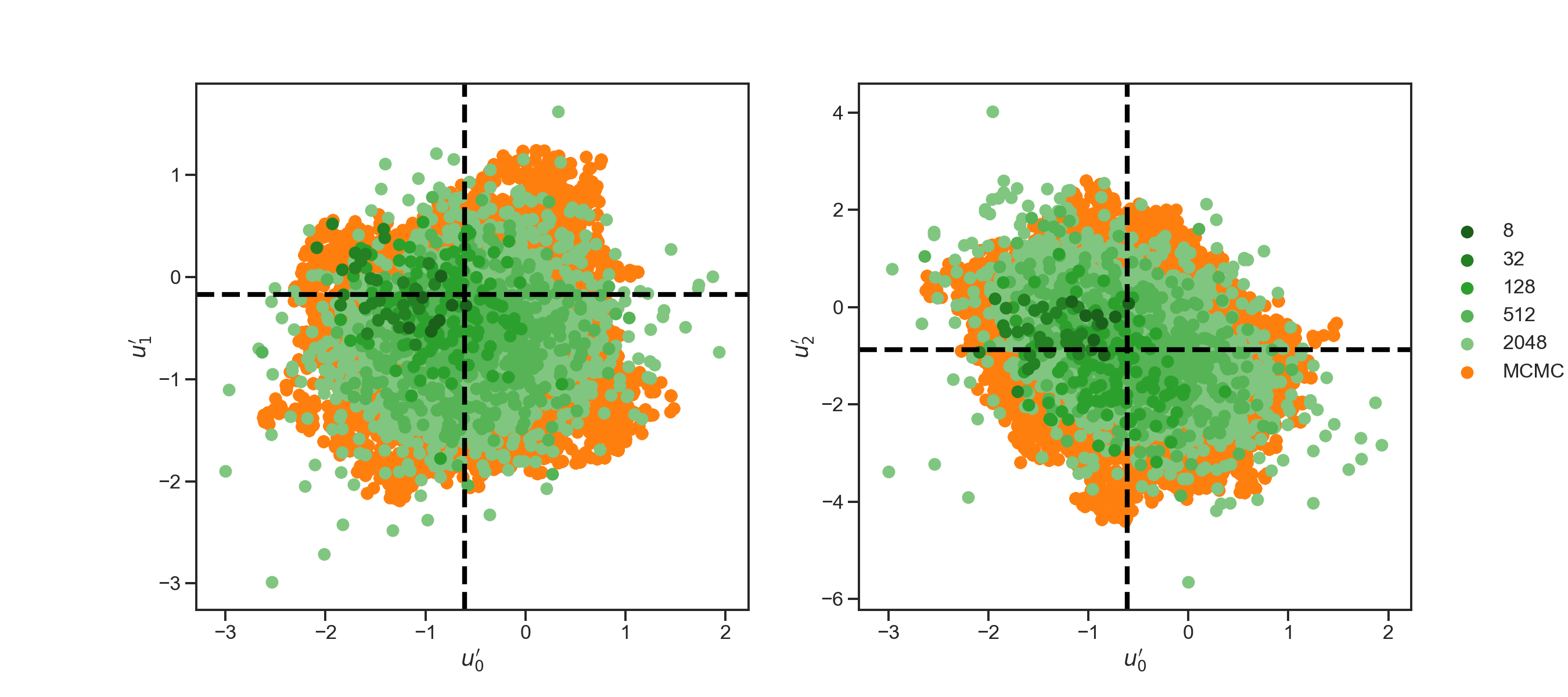 Figure 5
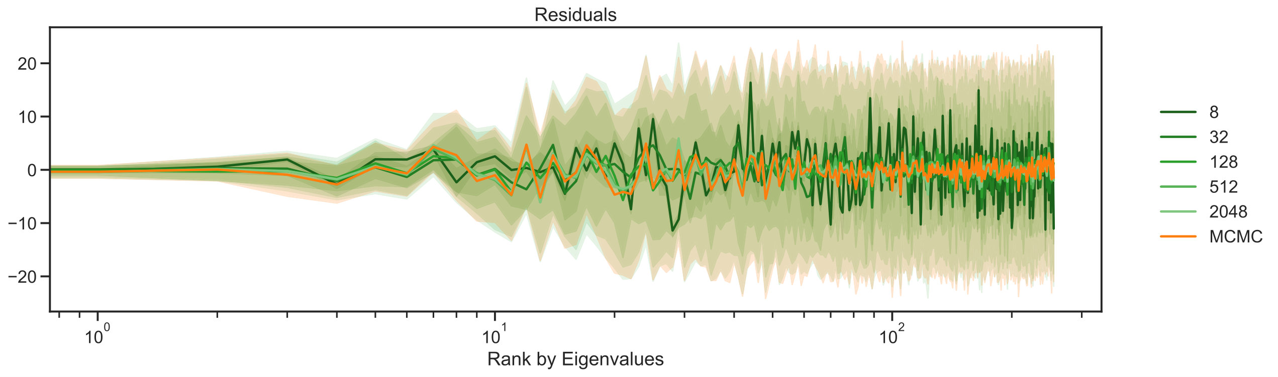 Figure 6
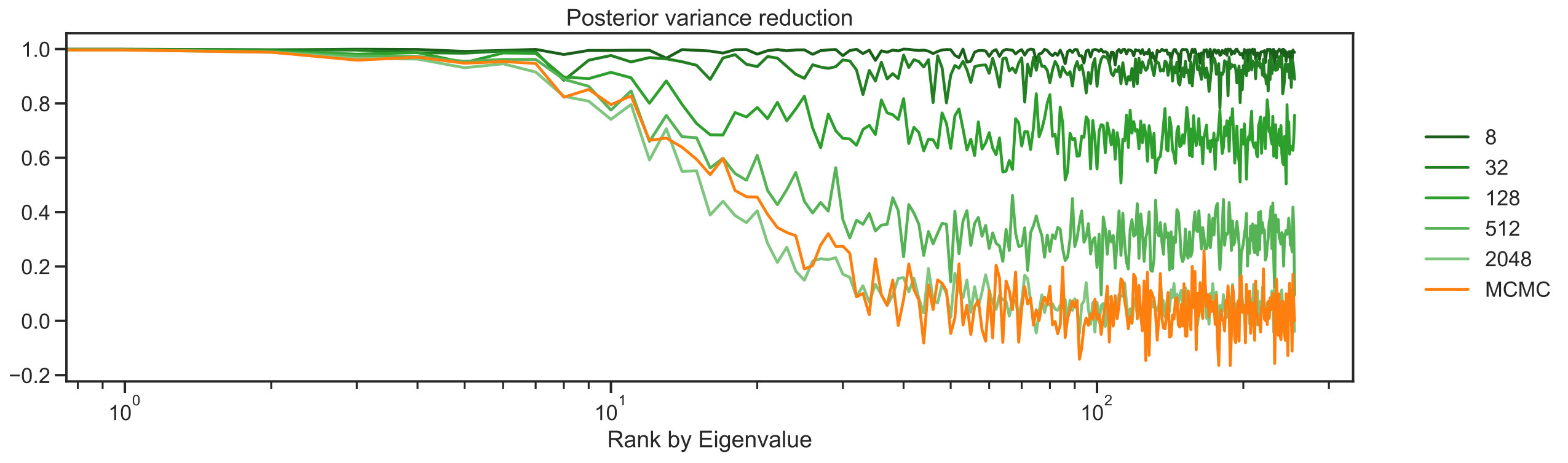 Figure 7
 Figure 8
 Figure 9
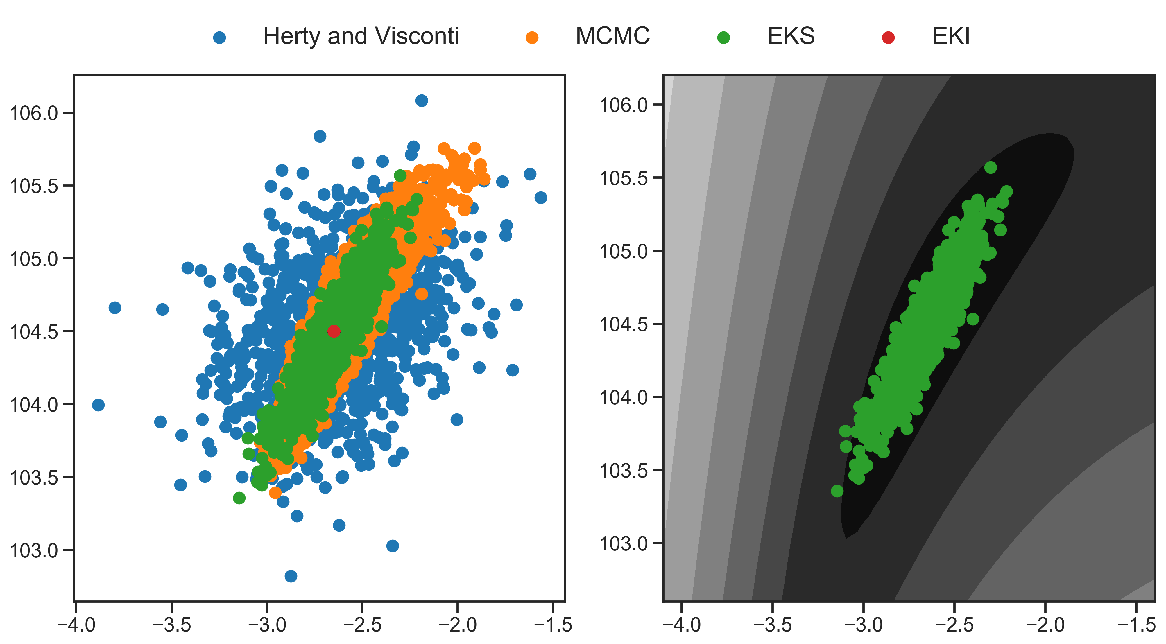 Figure 10
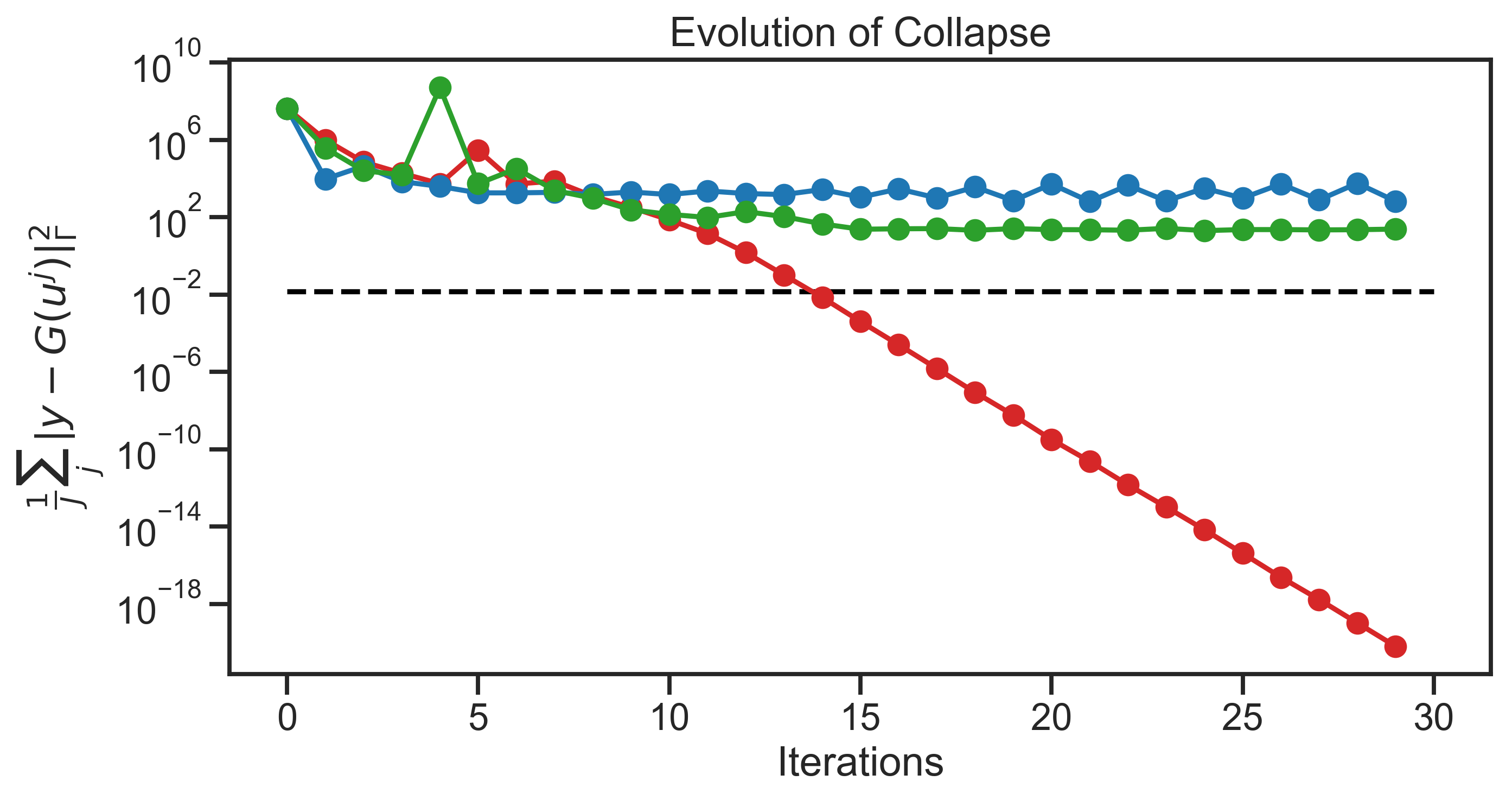 Figure 11
Peer Reviews
No public reviews on file for this paper yet. If you reviewed it on a platform where reviews are public (OpenReview, ICLR, NeurIPS, ICML), you can paste yours below so the community can read it here.
Videos
No videos yet. Explain this paper in a talk, walkthrough, or lecture? Add one.
\startlocaldefs\endlocaldefs
, ,
and
Interacting Langevin Diffusions: Gradient Structure And Ensemble Kalman Sampler
Alfredo Garbuno-Inigolabel=e1][email protected] [
Franca Hoffmannlabel=e2][email protected] [
Wuchen Lilabel=e3][email protected] [
Andrew M. Stuartlabel=e4][email protected] [ Department of Computing and Mathematical Sciences, Caltech, Pasadena, CA. e1,e2,e4
Department of Mathematics, UCLA, Los Angeles, CA. e3
Abstract
Solving inverse problems without the use of derivatives or adjoints of the forward model is highly desirable in many applications arising in science and engineering. In this paper we propose a new version of such a methodology, a framework for its analysis, and numerical evidence of the practicality of the method proposed. Our starting point is an ensemble of over-damped Langevin diffusions which interact through a single preconditioner computed as the empirical ensemble covariance. We demonstrate that the nonlinear Fokker-Planck equation arising from the mean-field limit of the associated stochastic differential equation (SDE) has a novel gradient flow structure, built on the Wasserstein metric and the covariance matrix of the noisy flow. Using this structure, we investigate large time properties of the Fokker-Planck equation, showing that its invariant measure coincides with that of a single Langevin diffusion, and demonstrating exponential convergence to the invariant measure in a number of settings. We introduce a new noisy variant on ensemble Kalman inversion (EKI) algorithms found from the original SDE by replacing exact gradients with ensemble differences; this defines the ensemble Kalman sampler (EKS). Numerical results are presented which demonstrate its efficacy as a derivative-free approximate sampler for the Bayesian posterior arising from inverse problems.
Keywords: Ensemble Kalman Inversion; Kalman–Wasserstein metric; Gradient flow; Mean-field Fokker-Planck equation.
1 Problem Setting
1.1 Background
Consider the inverse problem of finding from where
[TABLE]
is a known non-linear forward operator and is the unknown observational noise. Although itself is unknown, we assume that it is drawn from a known probability distribution; to be concrete we assume that this distribution is a centered Gaussian: for a known covariance matrix . In summary, the objective of the inverse problem is to find information about the truth underlying the data ; the forward map , the covariance and the data are all viewed as given.
A key role in any optimization scheme to solve (1.1) is played by for some loss function For additive Gaussian noise the natural loss function is 111For any positive-definite symmetric matrix we define and
[TABLE]
leading to the nonlinear least squares functional
[TABLE]
In the Bayesian approach to inversion (Kaipio and Somersalo, 2006) we place a prior distribution on the unknown , with Lebesgue density , then the posterior density on , denoted , is given by
[TABLE]
In this paper we will concentrate on the case where the prior is a centred Gaussian , assuming throughout that is strictly positive-definite and hence invertible. If we define
[TABLE]
and
[TABLE]
then
[TABLE]
Note that the regularization is of Tikhonov-Phillips form (Engl, Hanke and Neubauer, 1996).
Our focus throughout is on using interacting particle systems to approximate Langvein-type stochastic dynamical systems to sample from (1.6). Ensemble Kalman inversion (EKI), and variants of it, will be central in our approach because these methods play an important role in large-scale scientific and engineering applications in which it is undesirable, or impossible, to compute derivatives and adjoints defined by the forward map . Our goal is to introduce a noisy version of EKI which may be used to generate approximate samples from (1.6) based only on evaluations of , to exemplify its potential use and to provide a framework for its analysis. We refer to the new methodology as * ensemble Kalman sampling* (EKS).
1.2 Literature Review
The overdamped Langevin equation provides the simplest example of a reversible diffusion process with the property that it is invariant with respect to (1.6) (Pavliotis, 2014). It provides a conceptual starting point for a range of algorithms designed to draw approximate samples from the density (1.6). This idea may be generalized to non-reversible diffusions such as those with state-dependent noise (Duncan, Lelievre and Pavliotis, 2016), those which are higher order in time (Ottobre and Pavliotis, 2011) and combinations of the two (Girolami and Calderhead, 2011). In the case of higher order dynamics the desired target measure is found by marginalization. There are also a range of methods, often going under the collective names Nosé-Hoover-Poincaré, which identify the target measure as the marginal of an invariant measure induced by (ideally) chaotic and mixing deterministic dynamics (Leimkuhler and Matthews, 2016) or a mixture between chaotic and stochastic dynamics (Leimkuhler, Noorizadeh and Theil, 2009). Furthermore, the Langevin equation may be shown to govern the behaviour of a wide range of Monte Carlo Markov Chain (MCMC) methods; this work was initiated in the seminal paper (Roberts et al., 1997) and has given rise to many related works (Roberts and Rosenthal, 1998; Roberts et al., 2001; Bédard et al., 2007; Bedard, 2008; Bédard and Rosenthal, 2008; Mattingly et al., 2012; Pillai, Stuart and Thiéry, 2014; Ottobre and Pavliotis, 2011); for a recent overview see (Yang, Roberts and Rosenthal, 2019).
In this paper we will introduce an interacting particle system generalization of the overdamped Langevin equation, and use ideas from ensemble Kalman methodology to generate approximate solutions of the resulting stochastic flow, and hence approximate samples of (1.6), without computing dervatives of the log likelihood. The ensemble Kalman filter was originally introduced as a method for state estimation, and later extended as the EKI to the solution of general inverse problems and parameter estimation problems. For a historical development of the subject, the reader may consult the books (Evensen, 2009; Oliver, Reynolds and Liu, 2008; Majda and Harlim, 2012; Law, Stuart and Zygalakis, 2015; Reich and Cotter, 2015) and the recent review (Carrassi et al., 2018). The Kalman filter itself was derived for linear Gaussian state estimation problems (Kalman, 1960; Kalman and Bucy, 1961). In the linear setting, ensemble Kalman based methods may be viewed as Monte Carlo approximations of the Kalman filter; in the nonlinear case ensemble Kalman based methods do not converge to the filtering or posterior distribution in the large particle limit (Ernst, Sprungk and Starkloff, 2015). Related interacting particle based methodologies of current interest include Stein variational gradient descent (Lu, Lu and Nolen, 2018; Liu and Wang, 2016; Detommaso et al., 2018) and the Fokker-Planck particle dynamics of Reich (Reich, 2018; Pathiraja and Reich, 2019), both of which map an arbitrary initial measure into the desired posterior measure over an infinite time horizon . A related approach is to introduce an artificial time and a homotopy between the prior at time and the posterior measure at time and write an evolution equation for the measures (Daum and Huang, 2011; Reich, 2011; El Moselhy and Marzouk, 2012; Laugesen et al., 2015); this evolution equation can be approximated by particle methods. There are also other approaches in which optimal transport is used to evolve a sequence of particles through a transportation map (Reich, 2013; Marzouk et al., 2016) to solve probabilistic state estimation or inversion problems as well as interacting particle systems designed to reproduce the solution of the filtering problem (Crisan and Xiong, 2010; Yang, Mehta and Meyn, 2013). The paper (Del Moral et al., 2018) studies ensemble Kalman filters from the perspective of the mean-field process, and propagation of chaos. Also of interest are the consensus-based optimization techniques given a rigorous setting in (Carrillo et al., 2018).
The idea of using interacting particle systems derived from coupled Langevin-type equations is introduced within the context of MCMC methods in (Leimkuhler, Matthews and Weare, 2018); these methods require computation of derivatives of the log likelihood. In work (Duncan and Szpruch, 2019), concurrent with this paper, the interacting Langevin diffusions (2.3),(2.4) below are studied, the goal being to demonstrate that the pre-conditioning removes slow relaxation rates when they are present in the standard Langevin equation (2.1); such a result is proven in the case where the potential is quadratic and the posterior measure of interest is Gaussian. A key concept underlying both (Leimkuhler, Matthews and Weare, 2018) and (Duncan and Szpruch, 2019) is the idea of finding algorithms which converge to equilibrium at rates independent of the conditioning of the Hessian of the log posterior, an idea introduced in the affine invariant samplers of Goodman and Weare (2010).
Continuous-time limits of ensemble Kalman filters for state estimation were first introduced and studied systematically in the papers (Bergemann and Reich, 2012; Reich, 2011; Bergemann and Reich, 2010a, b); the papers (Bergemann and Reich, 2010a, b) studied the “analysis” step of filtering (using Bayes theorem to incorporate data) through introduction of an artificial continuous time; the papers (Bergemann and Reich, 2012; Reich, 2011) developed a seamless framework that integrated the true time for state evolution and the artificial time for incorporation of data into one. The resulting methodology has been studied in a number of subsequent papers, see (Del Moral, Kurtzmann and Tugaut, 2017; Del Moral et al., 2018; de Wiljes, Reich and Stannat, 2018; Taghvaei et al., 2018) and the references therein. A slightly different seamless continuous time formulation was introduced, and analyzed, a few years later in (Law, Stuart and Zygalakis, 2015; Kelly, Law and Stuart, 2014). Continuous time limits of ensemble methods for solving inverse problems were introduced and analyzed in the paper (Schillings and Stuart, 2017); in fact the work in the papers (Bergemann and Reich, 2010a, b) can be re-interpreted in the context of ensemble methods for inversion and also results in similar, but slightly different continuous time limits. The idea of iterating ensemble methods to solve inverse problems originated in the papers (Chen and Oliver, 2012; Emerick and Reynolds, 2013), which were focussed on applications in oil-reservoir applications; the paper (Iglesias, Law and Stuart, 2013) describes, and demonstrated the promise of, the methods introduced in those papers for quite general inverse problems. The specific continuous time version of the methodology, which we refer to as EKI in this paper, was identified in (Schillings and Stuart, 2017).
There has been significant activity devoted to the gradient flow structure associated with the Kalman filter itself. A well-known result is that for a constant state process, Kalman filtering is the gradient flow with respect to the Fisher-Rao metric (Laugesen et al., 2015; Halder and Georgiou, 2017; Ollivier, 2017). It is worth noting that the Fisher-Rao metric connects to the covariance matrix, see details in (Ay et al., 2017). On the other hand, optimal transport (Villani, 2009) demonstrates the importance of the -Wasserstein metric in probability density space. The space of densities equipped with this metric introduces an infinite-dimensional Riemannian manifold, called the density manifold (Lafferty, 1988; Otto, 2001; Li, 2018). Solutions to the Fokker-Planck equation are gradient flows of the relative entropy in the density manifold (Otto, 2001; Jordan, Kinderlehrer and Otto, 1998). Designing time-stepping methods which preserve gradient structure is also of current interest: see (Pathiraja and Reich, 2019) and, within the context of Wasserstein gradient flows, (Li and Montufar, 2018; Tong Lin et al., 2018; Li, Lin and Montúfar, 2019). The subject of discrete gradients for time-integration of gradient and Hamiltonian systems is developed in (Humphries and Stuart, 1994; Gonzalez, 1996; McLachlan, Quispel and Robidoux, 1999; Hairer and Lubich, 2013). Furthermore, the papers (Schillings and Stuart, 2017, ) study continuous time limits of EKI algorithms and, in the case of linear inverse problems, exhibit a gradient flow structure for the standard least squares loss function, preconditioned by the empirical covariance of the particles; a related structure was highlighted in (Bergemann and Reich, 2010a). The paper (Herty and Visconti, 2018), which has inspired aspects of our work, builds on the paper (Schillings and Stuart, 2017) to study the same problem in the mean-field limit; their mean-field perspective brings considerable insight which we build upon in this paper. Recent work (Ding and Li, 2019) has studied the approach to the mean-field limit for linear inverse problems, together with making connection to the appropriate nonlinear Fokker-Planck equation whose solution characterizes the distribution in the mean-field limit.
In this paper, we study a new noisy version of EKI, the ensemble Kalman sampler (EKS), and related mean-field limits, the aim being the construction of methods which lead to approximate posterior samples, without the use of adjoints, and overcoming the issue that the standard noisy EKI does not reproduce the posterior distribution, as highlighted in (Ernst, Sprungk and Starkloff, 2015). We emphasize that the practical derivative-free algorithm that we propose rests on a particle-based approximation of a specific preconditioned gradient flow, as described in section 4.3 of the paper (Kovachki and Stuart, 2018); we add a judiciously chosen noise to this setting and it is this additional noise which enables approximate posterior sampling. Related approximations are also studied in the paper (Pathiraja and Reich, 2019) in which the effect of both time-discretization and particle approximation are discussed when applied to various deterministic interacting particle systems with gradient structure. In order to frame the analysis of our methods, we introduce a new metric, named the Kalman-Wasserstein metric, defined through both the covariance matrix of the mean field limit and the Wasserstein metric. The work builds on the novel perspectives introduced in (Herty and Visconti, 2018) and leads to new algorithms that will be useful within large-scale parameter learning and uncertainty quantification studies, such as those proposed in (Schneider et al., 2017).
1.3 Our Contribution
The contributions in this paper are:
- •
We introduce a new noisy perturbation of the continuous time ensemble Kalman inversion (EKI) algorithm, leading to an interacting particle system in stochastic differential equation (SDE) form, the ensemble Kalman sampler (EKS).
- •
We also introduce a related SDE, in which ensemble differences are approximated by gradients; this approximation is exact for linear inverse problems. We study the mean-field limit of this related SDE, and exhibit a novel Kalman–Wasserstein gradient flow structure in the associated nonlinear Fokker-Planck equation.
- •
Using this Kalman–Wasserstein structure we characterize the steady states of the nonlinear Fokker-Planck equation, and show that one of them is the posterior density (1.6).
- •
By explicitly solving the nonlinear Fokker-Planck equation in the case of linear , we demonstrate that the posterior density is a global attractor for all initial densities of finite energy which are not a Dirac measure.
- •
We provide numerical examples which demonstrate that the EKS algorithm gives good approximate samples from the posterior distribution for both a simple low dimensional test problem, and for a PDE inverse problem arising in Darcy flow.
In Section 2 we introduce the various stochastic dynamical systems which form the basis for the proposed methodology and analysis: Subsection 2.1 describes an interacting particle system variant on Langevin dynamics; Subsection 2.2 recaps the EKI methodology, and describes the SDE arising in the case when the data is perturbed with noise; and Subsection 2.3 introduces the new noisy EKS algorithm, which arises from perturbing the particles with noise, rather than perturbing the data. In Section 3 we discuss the theoretical properties underpinning the proposed new methodology and in Section 4 we describe numerical results which demonstrate the value of the proposed new methodology. We conclude in Section 5.
2 Dynamical Systems Setting
This section is devoted to the various noisy dynamical systems that underpin the paper: in the three constituent subsections we introduce an interacting particle version of Langevin dynamics, the EKI algorithm and the new EKS algorithm. In so doing, we introduce a sequence of continuous time problems that are designed to either maximise the posterior distribution (EKI), or generate approximate samples from the posterior distribution (noisy EKI and the EKS). We then make a linear approximation within part of the EKS and take the mean-field limit leading to a novel nonlinear Fokker-Planck equation studied in the next section.
2.1 Variants On Langevin Dynamics
The overdampled Langevin equation has the form
[TABLE]
where W denotes a standard Brownian motion in 222In this SDE, and all that follow, the rigorous interpretation is through the Itô integral formulation of the problem. References to the relevant literature may be found in the introduction. A common approach to speed up convergence is to introduce a symmetric matrix in the corresponding gradient descent scheme,
[TABLE]
The key concept behind this stochastic dynamical system is that, under conditions on which ensure ergodicity, an arbitrary initial distribution is transformed into the desired posterior distribtion over an infinite time horizon.
To find a suitable matrix is of general interest. We propose to evolve an interacting set of particles according to the following system of SDEs:
[TABLE]
Here, the are a collection of i.i.d. standard Brownian motions in the space . The matrix depends non-linearly on all ensemble members, and is chosen to be the empirical covariance between particles,
[TABLE]
where denotes the sample mean
[TABLE]
This choice of preconditioning is motivated by an underlying gradient flow structure which we exhibit in Section 3.3. System (2.3) can be re-written as
[TABLE]
(We used the fact that it is possible to replace by after the weighted inner-product in (2.5) without changing the equation.) We will introduce an ensemble Kalman based methodology to approximate this interacting particle system, the EKS.
2.2 Ensemble Kalman Inversion
To understand the EKS we first recall the ensemble Kalman inversion (EKI) methodology which can be interpreted as a derivative-free optimization algorithm to invert (Iglesias, Law and Stuart, 2013; Iglesias, 2016). The continuous time version of the algorithm is given by (Schillings and Stuart, 2017):
[TABLE]
This interacting particle dynamic acts to both drive particles towards consensus and to fit the data. In (Chen and Oliver, 2012; Emerick and Reynolds, 2013) the idea of using ensemble Kalman methods to map prior samples into posterior samples was introduced (see the introduction for a literature review). Interpreted in our continuous time-setting, the methodology operates by evolving a noisy set of interacting particles given by
[TABLE]
where the are a collection of i.i.d. standard Brownian motions in the data space different choices of allow to remove noise and obtain an optimization algorithm () or to add noise in a manner which, for linear problems, creates a dynamic transporting the prior into the posterior in one time unit (, see discussion below).
Here, the operator denotes the empirical cross covariance matrix of the ensemble members,
[TABLE]
The approach is designed in the linear case to transform prior samples into posterior samples in one time unit (Chen and Oliver, 2012). In contrast to Langevin dynamics this has the desirable property that it works over a single time unit, rather than over an infinite time horizon. But it is considerably more rigid as it requires initialization at the prior. Furthermore, the long time dynamics do not have the desired sampling property, but rather collapse to a single point, solving the optimization problem of minimizing We now demonstrate these points by considering the linear problem.
To be explicit we consider the case where
[TABLE]
In this case, the regularized misfit equals
[TABLE]
The corresponding gradient can be written as
[TABLE]
The posterior mean is thus and the posterior covariance is
In the linear setting (2.9) and with the choice , the EKI algorithm defined in (2.7) has mean and covariance which satisfy the closed equations
[TABLE]
These results may be established by similar techniques to those used below in Subsection 3.2. (A more general analysis of the SDE (2.7), and its related nonlinear Fokker-Planck equation, is undertaken in (Ding and Li, 2019).) It follows that
[TABLE]
and therefore grows linearly in time. If the initial covariance is given by the prior then
[TABLE]
demonstrating that delivers the posterior covariance; furthermore it then follows that
[TABLE]
so that, initializing with prior mean we obtain
[TABLE]
and delivers the posterior mean.
The resulting equations for the mean and covariance are simply those which arise from applying the Kalman-Bucy filter (Kalman and Bucy, 1961) to the model
[TABLE]
where W denotes a standard unit Brownian motion in the data space The exact closed form of equations for the first two moments, in the setting of the Kalman-Bucy filter, was established in Section 4 of the paper (Reich, 2011) for finite particle approximations, and transfers verbatim to this mean-field setting.
The analysis reveals interesting behaviour in the large time limit: the covariance shrinks to zero and the mean converges to the solution of the unregularized least squares problem; we thus have ensemble collapse and solution of an optimization problem, rather than a sampling problem. This highights an interesting perspective on the EKI, namely as an optimization method rather than a sampling method. A key point to appreciate is that the noise introduced in (2.7) arises from the observation being perturbed with additional noise. In what follows we instead directly perturb the particles themselves. The benefits of introducing noise on the particles, rather than the data, was demonstrated in (Kovachki and Stuart, 2018), although in that setting only optimization, and not Bayesian inversion, is considered.
2.3 The Ensemble Kalman Sampler
We now demonstrate how to introduce noise on the particles within the ensemble Kalman methodology, with our starting point being (2.5). This gives the EKS. In contrast to the standard noisy EKI (2.7), the EKS is based on a dynamic which transforms an arbitrary initial distribution into the desired posterior distribution, over an infinite time horizon. In many applications, derivatives of the forward map are either not available, or extremely costly to obtain. A common technique used in ensemble Kalman methods is to approximate the gradient by differences in order to obtain a derivative-free algorithm for inverting . To this end, consider the dynamical system (2.5) and invoke the approximation
[TABLE]
This leads to the following derivative-free algorithm to generate approximate samples from the posterior distribution,
[TABLE]
This dynamical system is similar to the noisy EKI (2.7) but has a different noise structure (noise in parameter space not data space) and explicitly accounts for the prior on the right hand side (rather than having it enter through initialization). Inclusion of the Tikhonov regularization term within EKI is introduced and studied in (Chada, Stuart and Tong, 2019).
Note that in the linear case (2.9) the two systems (2.5) and (2.13) are identical. It is also natural to conjecture that if the particles are close to one another then (2.5) and (2.13) will generate similar particle distributions. Based on this exact (in the linear case) and conjectured (in the nonlinear case) relationship we propose (2.13) as a derivative-free algorithm to approximately sample the Bayesian posterior distribution, and we propose (2.5) as a natural object of analysis in order to understand this sampling algorithm.
2.4 Mean Field Limit
In order to write down the mean field limit of (2.5), we define the macroscopic mean and covariance:
[TABLE]
Taking the large particle limit leads to the mean field equation
[TABLE]
with corresponding nonlinear Fokker-Planck equation
[TABLE]
Here denotes the Frobenius inner-product between matrices and . The existence and form of the mean-field limit is suggested by the exchangeability of the process (existence) and by application of the law of large numbers (form). Exchangeability is exploited in a related context in (Del Moral, Kurtzmann and Tugaut, 2017; Del Moral et al., 2018). The rigorous derivation of the mean-field equations (2.14) and (2.15) is left for future work; for foundational work relating to mean field limits, see (Sznitman, 1991; Jabin and Wang, 2017; Carrillo et al., 2010; Ha and Tadmor, 2008; Pareschi and Toscani, 2013; Toscani, 2006) and the references therein. The following lemma states the intuitive fact that the covariance, which plays a central role in equation (2.15), vanishes only for Dirac measures.
Lemma 1**.**
The only probability densities at which vanishes are Diracs,
[TABLE]
Proof.
That follows by direct substitution. For the converse, note that implies , which is the equality case of Jensen’s inequality, and therefore only holds if is the law of a constant random variable. ∎
3 Theoretical Properties
In this section we discuss theoretical properties of (2.15) which motivate the use of (2.5) and (2.13) as particle systems to generate approximate samples from the posterior distribution (1.6). In Subsection 3.1 we exhibit a gradient flow structure for (2.15) which shows that solutions evolve towards the posterior distribution (1.6) unless they collapse to a Dirac measure. In Subsection 3.2 we show that in the linear case, collapse to a Dirac does not occur if the initial condition is a Gaussian with non-zero covariance, and instead convergence to the posterior distribution is obtained. In Subsection 3.3 we introduce a novel metric structure which underpins the results in the two preceding sections, and will allow for a rigorous analysis of the long-term behavior of the nonlinear Fokker-Planck equation in future work.
3.1 Nonlinear Problem
Because is independent of , we may write equation (2.15) in divergence form, which facilitates the revelation of a gradient structure:
[TABLE]
where we use the fact . Indeed, equation (3.1) is nothing but the Fokker-Planck equation for (2.2) for a time-dependent matrix . Thanks to the divergence form, it follows that (3.1) conserves mass along the flow, and so we may assume for all . Defining the energy
[TABLE]
solutions to (3.1) can be written as a gradient flow:
[TABLE]
where denotes the first variation. This will be made more explicit in Section 3.3, see Proposition 7. Thanks to the gradient flow structure (3.3), stationary states of (2.15) are given either by critical points of the energy , or by choices of such that as characterized in Lemma 1. Critical points of solve the corresponding Euler-Lagrange condition
[TABLE]
for some constant . The unique solution to (3.4) with unit mass is given by the Gibbs measure
[TABLE]
Then, up to an additive normalization constant, the energy is exactly the relative entropy of with respect to , also known as the Kullback-Leibler divergence ,
[TABLE]
Thanks to the gradient flow structure (3.3), we can compute the dissipation of the energy
[TABLE]
As a consequence, the energy decreases along trajectories until either approaches zero (collapse to a Dirac measure by Lemma 1) or becomes the Gibbs measure with density .
The dissipation of the energy along the evolution of the classical Fokker-Planck equation is known as the Fisher information (Villani, 2009). We reformulate equation (3.6) by defining the following generalized Fisher information for any covariance matrix ,
[TABLE]
One may also refer to as a Dirichlet form as it is known in the theory of large particle systems, since we can write
[TABLE]
For , we name functional the relative Kalman-Fisher information. We conclude that the following energy dissipation equality holds,
[TABLE]
To derive a rate of decay to equilibrium in entropy, we aim to identify conditions on such that the following logarithmic Sobolev inequality holds: there exists such that
[TABLE]
By (Bakry and Émery, 1985), it is enough to impose sufficient convexity on , i.e. , where denotes the Hessian of . This allows us to deduce convergence to equilibrium as long as is uniformly bounded from below following standard arguments for the classical Fokker-Planck equation as presented for example in (Markowich and Villani, 2000).
Proposition 2**.**
Assume there exists and such that
[TABLE]
Then any solution to (3.1) with initial condition satisfying decays exponentially fast to equilibrium: there exists a constant such that for any ,
[TABLE]
This rate of convergence can most likely be improved using the correct logarithmic Sobolev inequality weighted by the covariance matrix . However, the above estimate already indicates the effect of having the covariance matrix present in the Fokker-Planck equation (3.1). The properties of such inequalities in a more general setting is an interesting future avenue to explore. The weighted logarithmic Sobolev inequality that is well adapted to the setting here depends on the geometric structure of the Kalman-Wasserstein metric, see related studies in (Li, 2018).
Proof.
Thanks to the assumptions, and using the logarithmic Sobolev inequality (3.7), we obtain decay in entropy,
[TABLE]
We conclude using the Csiszár-Kullback inequality as it is mainly known to analysts, also referred to as Pinsker inequality in probability (see (Arnold et al., 2001) for more details):
[TABLE]
∎
3.2 Linear Problem
Here we show that, in the case of a linear forward operator , the Fokker-Planck equation (which is still nonlinear) has exact Gaussian solutions. This property may be seen to hold in two ways: (i) by considering the case in which the covariance matrix is an exogenously defined function of time alone, in which case the observation is straightforward; and (ii) because the mean field equation (2.14) leads to exact closed equations for the mean and covariance. Once the covariance is known the nonlinear Fokker-Planck equation (2.15) becomes linear, and is explicitly solvable if is linear and the initial condition is Gaussian. Consider equation (2.14) in the context of a linear observation map (2.9). The misfit is given by (2.10), and the gradient of is given in (2.11). Note that since we assume that the covariance matrix is invertible, it is then also strictly positive-definite. Thus it follows that is strictly positive-definite and hence invertible too. We define noting that this is the solution of the regularized normal equations defining the minimizer of in this linear case; equivalently maximizes the posterior density. Indeed by completing the square we see that we may write
[TABLE]
Lemma 3**.**
Let be a solution of (2.15) with given by (2.10). Then the mean and covariance matrix are determined by and which satisfy the evolution equations
[TABLE]
In addition, for any satisfying (3.9b), its determinant and inverse solve
[TABLE]
[TABLE]
As a consequence and exponentially as .
In fact, solving the ODE (3.11) explicitly and using (3.9a), exponential decay immediately follows:
[TABLE]
and
[TABLE]
Proof.
We begin by deriving the evolution of the first and second moments. This is most easily accomplished by working with the mean-field flow SDE (2.14), using the regularized linear misfit written in (2.10). This yields the update
[TABLE]
where denotes a zero mean random variable. Identical results can be obtained by working directly with the PDE for the density, namely (2.15) with the regularized linear misfit given in (2.10). Taking expectations with respect to results in
[TABLE]
Let us use the following auxiliary variable . By linearity of differentiation we can write
[TABLE]
By definition of the covariance operator, , its derivative with respect to time can be written as
[TABLE]
However we must also include the Itô correction, using Itô’s formula, and we can write the evolution equation of the covariance operator as
[TABLE]
This concludes the proof of (3.9b). For the evolution of the determinant and inverse, note that
[TABLE]
and so (3.10), (3.11) directly follow. Finally, exponential decay is a consequence of the explicit expressions (3.12) and (3.13). ∎
Thanks to the evolution of the covariance matrix and its determinant, we can deduce that there is a family of Gaussian initial conditions that stay Gaussian along the flow and converge to the equilibrium .
Proposition 4**.**
Fix a vector , a matrix and take as initial density the Gaussian distribution
[TABLE]
with mean and covariance . Then the Gaussian profile
[TABLE]
solves evolution equation (2.15) with initial condition , and where and evolve according to (3.9a) and (3.9b) with initial conditions and . As a consequence, for such initial conditions , the solution of the Fokker-Planck equation (2.15) converges to given by (3.8) as
Proof.
It is straightforward to see that, for and given by Lemma 3,
[TABLE]
since both and are independent of . Therefore, substituting the Gaussian ansatz into the first term in the right hand side of (2.15), we have
[TABLE]
where , and . Recall that is invertible. The second term on the right hand side of (2.15) can be simplified, as follows
[TABLE]
Thus, combining the previous two equations, the right hand side of (2.15) is given by the following expression
[TABLE]
For the left-hand side of (2.15), note that by (3.9a) and (3.9b),
[TABLE]
and therefore, combining with (3.10),
[TABLE]
which concludes the first part of the proof. The second part concerning the large time asymptotics is a straightforward consequence of the asymptotic behaviour of and detailed in Lemma 3. ∎
In the case of the classical Fokker-Planck equation with a quadratic confining potential, the result in Proposition 4 follows from the fact that the fundamental solution of (2.15) is a Gaussian, see (Carrillo and Toscani, 1998).
Corollary 5**.**
Let be a non-Gaussian initial condition for (2.15) in the case where is given by (2.10). Assume that satisfies . Then any solution of (2.15) converges exponentially fast to given by (3.5) as both in entropy, and in .
Proof.
Let have Euclidean norm and define . From equation (3.11) it follows that
[TABLE]
where is the maximum eigenvalue of . Hence it follows that is bounded above, independently of , and that hence is bounded from below as an operator. Together with the fact that the Hessian is bounded from below, we conclude using Proposition 2. ∎
3.3 Kalman-Wasserstein Gradient Flow
We introduce an infinite-dimensional Riemannian metric structure, which we name the Kalman-Wasserstein metric, in density space. It allows the interpretation of solutions to equation (2.15) as gradient flows in density space. To this end we denote by the space of probability measures on a convex set :
[TABLE]
The probability simplex is a manifold with boundary. For simplicity, we focus on the subset
[TABLE]
The tangent space of at a point is given by
[TABLE]
The second equality follows since for all we have as the mass along all curves in remains constant. For the set , the tangent space is therefore independent of the point . Cotangent vectors are elements of the topological dual and can be identified with tangent vectors via the action of the Onsager operator (Mielke, Peletier and Renger, 2016; Onsager, 1931a, b; Machlup and Onsager, 1953; Öttinger, 2005)
[TABLE]
In this paper, we introduce the following new choice of Onsager operator:
[TABLE]
By Lemma 1, the weighted elliptic operator becomes degenerate if is a Dirac. For points in the set that are bounded away from zero, the operator is well-defined, non-singular and invertible since . So we can write
[TABLE]
This provides a 1-to-1 correspondence between elements and . For general , we can instead use the pseudo-inverse , see (Li, 2018). With the above choice of Onsager operator, we can define a generalized Wasserstein metric tensor:
Definition 6** (Kalman-Wasserstein metric tensor).**
Define
[TABLE]
as follows:
[TABLE]
where for .
With this metric tensor, the Kalman-Wasserstein metric can be represented by the geometric action function. Given two densities , , consider
[TABLE]
where the infimum is taken among all continuous density paths and potential functions . The Kalman-Wasserstein metric has several interesting mathematical properties, which will be the focus of future work. In this paper, working in , we derive the gradient flow formulation that underpins the formal calculations given in Subsection 3.1 for the energy functional defined in (3.2).
Proposition 7**.**
Given a finite functional , the gradient flow of in satisfies
[TABLE]
Proof.
The Riemannian gradient operator is defined via the metric tensor as follows:
[TABLE]
Thus, for , we have
[TABLE]
Hence
[TABLE]
Thus we derive the gradient flow by
[TABLE]
∎
Remark 8**.**
Our derivation concerns the gradient flow on the subset of for simplicity of exposition. However, a rigorous analysis of the evolution of the gradient flow (3.3) requires to extend the above arguments to the full set of probabilities , especially as we want to study Dirac measures in view of Lemma 1. If is an element of the boundary of , one may consider instead the pseudo inverse of the operator . This will be the focus of future work, also see the more general analysis in (Ambrosio, Gigli and Savaré, 2005), e.g. Theorem 11.1.6.
4 Numerical Experiments
In this section we demonstrate that the intuition developed in the previous two sections does indeed translate into useful algorithms for generating approximate posterior samples without computing derivatives of the forward map . We do this by considering non-Gaussian inverse problems, defined through a nonlinear forward operator , showing how numerical solutions of (2.13) are distributed after large time, and comparing them with exact posterior samples found from MCMC.
Achieving the mean-field limit requires large, and hence typically larger than the dimension of the parameter space. There are interesting and important problems arising in science and engineering in which the number of parameters to be estimated is small, even though evaluation of involves solution of computationally expensive PDEs; in this case choosing is not prohibitive. We also include numerical results which probe outcomes when To this end we study two problems, the first an inverse problem for a two-dimensional vector arising from a two point boundary-value problem, and the second an inverse problem for permeability from pressure measurements in Darcy flow; in this second problem the dimension of the parameter space is tunable from small up to infinite dimension, in principle.
4.1 Derivative-Free
In this subsection we describe how to use (2.13) for the solution of the inverse problem (1.1). We approximate the continuous time stochastic dynamics by means of a linearly implicit split-step discretization scheme given by
[TABLE]
where , is the prior covariance and is an adaptive timestep computed as in (Kovachki and Stuart, 2018).
4.2 Gold Standard: MCMC
In this subsection we describe the specific Random Walk Metropolis Hastings (RWMH) algorithm used to solve the same Bayesian inverse problem as in the previous subsection; we view the results as gold standard samples from the desired posterior distribution. The link between RWMH methods and Langevin sampling is explained in the literature review within the introduction where it is shown that the latter arises as a diffusion limit of the former, as shown in numerous papers following on from the seminal work in (Roberts et al., 1997). The proposal distribution is a Gaussian centered at the current state of the Markov chain with covariance given by , where is the covariance computed from the last iteration of the algorithm described in the preceding subsection, and is a scaling factor tuned for an acceptance rate of approximately (Roberts et al., 1997). In our case, . The RWMH algorithm was used to get samples with the Markov chain starting at an approximate solution given by the mean of the last step of the algorithm from the previous subsection. For the high dimensional problem we use the pCN variant on RWMH (Cotter et al., 2013); this too has a diffusion limit of Langevin form (Pillai, Stuart and Thiéry, 2014).
4.3 Numerical Results: Low Dimensional Parameter Space
The numerical experiment considered here is the example originally presented in (Ernst, Sprungk and Starkloff, 2015) and also used in (Herty and Visconti, 2018). We start by defining the forward map which is given by the one-dimensional elliptic boundary value problem
[TABLE]
with boundary conditions and . The explicit solution for this problem, (see Herty and Visconti, 2018), is given by
[TABLE]
The forward model operator is then defined by
[TABLE]
Here is a constant vector that we want to find and we assume that we are given noisy measurements of at locations and . The precise Bayesian inverse problem considered here is to find the distribution of the unknown conditioned on the observed data , assuming additive Gaussian noise , where and is the identity matrix. We use as prior distribution , with The resulting Bayesian inverse problem is then solved, approximately, by the algorithms we now outline and with with observed data . Following (Herty and Visconti, 2018), we consider an initial ensemble drawn from .
Figure 1 shows the results for the solution of the Bayesian inverse problem considered above. In addition to implementing the algorithms described in the previous two subsections, we also employ a specific implementation of the EKI formulation introduced in the paper of Herty and Visconti (2018), and defined by the numerical discretization shown in (4.1), but with replaced by the identity matrix ; this corresponds to the algorithm from equation (20) of Herty and Visconti (2018), and in particular the last display of their Section 5, with The blue dots correspond to the output of this algorithm at the last iteration. The red dots correspond to the last ensemble of the EKI algorithm as presented in (Kovachki and Stuart, 2018). The orange dots depict the RWMH gold standard described above. Finally, the green dots shows the ensemble members at the last iteration of the proposed EKS (2.13). In this experiment, all versions of the ensemble Kalman methods were run with the adaptive timestep scheme from Subsection 4.1 and all were run for iterations with an ensemble size of .
Consider first the top-left panel. The true distribution, computed by RWMH, is shown in orange. Note that the algorithm of Kovachki and Stuart (2018) collapses to a point (shown in red), unable to escape overfitting, and relating to a form of consensus formation. In contrast, the algorithm of Herty and Visconti (2018), while avoiding overfitting, overestimates the spread of the ensemble members, relative to the gold standard RWMH; this is exhibited by the blue over-dispersed points. The proposed EKS (green points) gives results close to the RWMH gold standard. These issues are further demonstrated in the lower panel which shows the misfit (loss) function as a function of iterations for the three algorithms (excluding RWMH); the red line demonstrates overfitting as the misfit value falls below the noise level, whereas the other two algorithms avoid overfitting.
We include the derivative-free optimization algorithm EKI (red points) because it gives insight into what can be achieved with these ensemble based methods in the absence of noise (namely derivative-free optimization); we include the noisy EKI algorithm of Herty and Visconti (2018) (blue points) to demonstrate that considerable care is needed with the introduction of noise if the goal is to produce posterior samples; and we include our proposed EKS algorithm (green points) to demonstrate that judicious addition of noise to the EKI algorithm helps to produce approximate samples from the true posterior distribution of the Bayesian inverse problem; we include true posterior samples (orange points) for comparison. We reiterate that the methods of Chen and Oliver (2012); Emerick and Reynolds (2013) also hold the potential to produce good approximate samples, though they suffer from the rigidity of needing to be initialized at the prior and integrated to exactly time .
4.4 Numerical Results: High Dimensional Parameter Space
The forward problem of interest is to find the pressure field in a porous medium defined by permeability field ; for simplicity we assume that is a scalar-field in this paper. Given a scalar field defining sources and sinks of fluid, and assuming Dirichlet boundary conditions on the pressure for simplicity, we obtain the following elliptic PDE for the pressure:
[TABLE]
In what follows we will work on the domain We assume that the permeability is dependent on unknown parameters , so that The inverse problem of interest is to determine from linear functionals (measurements) of , subject to additive noise. Thus
[TABLE]
We will assume that so that and thus we take the to be linear functionals on the space . In practice we will work with pointwise measurements so that ; these are not elements of the dual space of in dimension ; but mollifications of them are, and in practice mollification with a narrow kernel does not affect results of the type presented here and so we do not use it (Iglesias, 2015). We model as a log-Gaussian field with precision operator defined as
[TABLE]
where the Laplacian is equipped with Neumann boundary conditions on the space of spatial-mean zero functions, and and are known constants that control the underlying lengthscales and smoothness of the underlying random field. In our experiments , and Such parametrization yields a Karhunen-Loève (KL) expansion
[TABLE]
where the eigenpairs are of the form
[TABLE]
where is the set of indices over which the random series is summed and the i.i.d. (Pavliotis, 2014). In pratice we will approximate by , a set with finite cardinality , and consider different For visualization we will sometimes find it helpful to write (4.10) as a sum over a one-dimensional variable rather than a lattice:
[TABLE]
We order the indices in so that the eigenvalues are in descending order by size.
We generate a truth random field by constructing by sampling it from , with and the identity on and using as the coefficients in (4.10). We create data from (1.1) with For the Bayesian inversion we choose prior covariance we also sample from this prior to initialize the ensemble for EKS. We run the experiments with different ensemble sizes to understand both strengths and limitations of the proposed algorithm for nonlinear forward models. Finally, we chose which allows the study of both and within the methodology.
Results showing the solution of this Bayesian inverse problem by MCMC (orange dots), with samples, and by the EKS with different (different shades of green dots) are shown in fig. 2 and fig. 3. For every ensemble size configuration, the EKS algorithm was run until units of time were achieved. As can be seen from fig. 2(b) the algorithm has reached an equilibrium after this duration. The two dimensional scatter plots in figure 2(a) show components with . That is, we are showing the components of which are associated to the three largest eigenvalues in the KL expansion (4.10) under the posterior distribution. We can see that sample spread is better matched to the gold standard MCMC spread as the size of the EKS ensemble is increased. In fig. 2(b) and fig. 2(c) we show the evolution of the dispersion of the ensemble around its mean at every time step, , and around the truth . The metrics we use to test the ensemble spread are
[TABLE]
where both are evaluated at and at every simulated time . For these metrics we use the norms defined by
[TABLE]
where the first is defined in the negative Sobolev space , whilst the second in the space. The first norm allows for higher discrepancy in the estimation of the tail of the modes in equation (4.10). Whereas, the second norm penalizes equally discrepancies in the tail of the KL expansion. In fig. 2(b), we see rapid convergence of the spread around the mean and around the truth for all ensmeble sizes The evolution in fig. 2(b) for both cases shows that the algorithm reaches its stationary distribution, while incorporating higher variability with increasing ensemble size. The figures are similar because the posterior mean and the truth are close to one another. Lower values of the metrics in fig. 2(b) and fig. 2(c) for smaller ensembles can be understood due to a mixed effect of reduced variability and overfitting to the MAP estimate of the Bayesian inverse problem. The results using the norm in fig. 2(c), allows us to see more discrepancy between ensemble sizes. Higher metric value for larger ensembles is due to the ensemble better approximating the posterior, as will be discussed below. In summary, fig. 2 shows evidence that the EKS is generating samples from a good approximation to the posterior and that this posterior is centred close to the truth. Increasing the ensemble size improves these features of the EKS method.
Figure 3 demonstrates how different ensemble sizes are able to capture the marginal posterior variances of each component in the unkown . The top panel in Figure 3 tracks the posterior variance reduction statistic for every component of which as mentioned before, now is viewed as a vector of components rather than a function on subset of the two-dimensional lattice. The posterior variance reduction is a measure of the relative decrease of variance for a given quantity of interest under the posterior with respect to the prior. It is defined as
[TABLE]
where denotes the variance of a random variable. The summary statistic has been used in (Spiegelhalter et al., 2002) to estimate the effective number of parameters in Bayesian models. When this parameter is close to then the algorithm has reduced uncertainty considerably, relative to the prior; when it is close to zero it has reduced it very little, in comparison with the prior. By studying the figure for the MCMC algorithm (orange) and comparing with EKS for increasing (green) we see that for around the match between EKS and MCMC is excellent. We also see that for smaller-sized ensembles there is a regularizing effect which artificially reduces the posterior variation for larger On the other hand, the lower panel in Figure 3 allows us to identify the location of ensemble density by plotting the residuals , for every component ; in particular we plot the algorithmic mean of this quantity and confidence intervals. It can be seen that the ensemble is well located as most of the components include the zero horizontal line, meaning that marginally the distribution of every component includes the correct value with high probability. Moreover, we can see two effects in this figure. Firstly, the lower variability in the first components also shows that there is enough information on the observed data to identify these components. Secondly, it can be seen that for very low-sized ensembles the least important components of incorporate higher error, when comparing the EKS samples in green with the orange MCMC samples.
Overall, the mismatch between the results from EKS and the MCMC reference in both numerical examples can be understood from the fact that the use of the ensemble equations (2.13) introduces a linear approximation to the curvature of the regularized misfit. This effect is demonstrated clearly in Figure 1, which shows the samples from EKS against a background of the level sets of the posterior. However, despite this mismatch, the key point is that a relatively good set of approximate samples in green is computed without use of the derivative of the forward model in both numerical examples; it thus holds promise as a method for large-scale nonlinear inverse problems.
5 Conclusions
In this paper we have demonstrated a methodoogy for the addition of noise to the basic EKI algorithm so that it generates approximate samples from the Bayesian posterior distribution – the ensemble Kalman sampler (EKS). Our starting point is a set of interacting Langevin diffusions, preconditioned by their mutual empirical covariance. To understand this system we introduce a new mean-field Fokker-Planck equation which has the desired posterior distribution as an invariant measure. We exhibit the new Kalman-Wasserstein metric with respect to which the Fokker-Planck equation has gradient structure. We also show how to compute approximate samples from this model by using a particle approximation based on using ensemble differences in place of gradients, leading to the EKS algorithm.
In the future we anticipate that methodology to correct for the error introduced by use of ensemble differences will be a worthwhile development from the algorithms proposed and we are actively pursuing this (Cleary et al., 2019). Furthermore, recent interesting work of Nüsken and Reich (2019) studies the invariant measures of the finite particle system (2.3), (2.4). The authors identify a simple linear correction term of order in (2.3) which renders the fold product of the posterior distribution invariant for finite ensemble number; since one of the major motivations for the use of ensemble methods is their robustness for small , this correction is important.
We also recognize that other difference-based methods for approximating gradients may emerge and that developing theory to quantify and control the errors arising from such difference approximations will be of interest. We believe that our proposed ensemble-based difference approximation is of particular value because of the growing community of scientists and engineers who work directly with ensemble based methods, because of their simplicity and black-box nature. In the future, we will also study the properties of the Kalman-Wasserstein metric including its duality, geodesics, and geometric structure, a line of research that is of independent mathematical interest in the context of generalized Wasserstein-type spaces. We will investigate the analytical properties of the new metric within Gaussian families. We expect these studies will bring insights to design new numerical algorithms for the approximate solution of inverse problems.
Acknowledgements: The authors are grateful to José A. Carrillo, Greg Pavliotis and Sebastian Reich for helpful input which improved this paper. A.G.I. and A.M.S. are supported by the generosity of Eric and Wendy Schmidt by recommendation of the Schmidt Futures program, by Earthrise Alliance, by the Paul G. Allen Family Foundation, and by the National Science Foundation (NSF grant AGS‐1835860). A.M.S. is also supported by NSF under grant DMS 1818977. F.H. was partially supported by Caltech’s von Karman postdoctoral instructorship. W.L. was supported by AFOSR MURI FA9550-18-1-0502.
The reference list from the paper itself. Each links out to its DOI / PubMed record.
- 1Ambrosio, Gigli and Savaré (2005) {bmisc} [author] \bauthor \bsnm Ambrosio, \bfnm Luigi \binits L., \bauthor \bsnm Gigli, \bfnm Nicola \binits N. and \bauthor \bsnm Savaré, \bfnm Giuseppe \binits G. ( \byear 2005). \btitle Gradient Flows: In Metric Spaces and in the Space of Probability Measures. \endbibitem
- 2Arnold et al. (2001) {barticle} [author] \bauthor \bsnm Arnold, \bfnm Anton \binits A., \bauthor \bsnm Markowich, \bfnm Peter \binits P., \bauthor \bsnm Toscani, \bfnm Giuseppe \binits G. and \bauthor \bsnm Unterreiter, \bfnm Andreas \binits A. ( \byear 2001). \btitle On convex Sobolev inequalities and the rate of convergence to equilibrium for Fokker-Planck type equations. \bjournal Comm. Partial Differential Equations \bvolume 26 \bpages 43–100. \bdoi 10.1081/PDE-100002246 \
- 3Ay et al. (2017) {bbook} [author] \bauthor \bsnm Ay, \bfnm Nihat \binits N., \bauthor \bsnm Jost, \bfnm Jürgen \binits J., \bauthor \bsnm Lê, \bfnm Hông Vân \binits H. V. and \bauthor \bsnm Schwachhöfer, \bfnm Lorenz Johannes \binits L. J. ( \byear 2017). \btitle Information Geometry. \bseries Ergebnisse Der Mathematik Und Ihrer Grenzgebiete A @series of Modern Surveys in Mathematics$l 3. Folge, Volume 64. \bpublisher Springer, \baddress Cham. \endbibitem
- 4Bakry and Émery (1985) {bincollection} [author] \bauthor \bsnm Bakry, \bfnm D. \binits D. and \bauthor \bsnm Émery, \bfnm Michel \binits M. ( \byear 1985). \btitle Diffusions hypercontractives. In \bbooktitle Séminaire de probabilités, XIX, 1983/84. \bseries Lecture Notes in Math. \bvolume 1123 \bpages 177–206. \bpublisher Springer, Berlin. \bdoi 10.1007/B Fb 0075847 \bmrnumber 889476 \endbibitem
- 5Bedard (2008) {barticle} [author] \bauthor \bsnm Bedard, \bfnm Mylene \binits M. ( \byear 2008). \btitle Optimal acceptance rates for Metropolis algorithms: Moving beyond 0.234. \bjournal Stochastic Processes and their Applications \bvolume 118 \bpages 2198–2222. \endbibitem
- 6Bédard et al. (2007) {barticle} [author] \bauthor \bsnm Bédard, \bfnm Mylene \binits M. \betal et al. ( \byear 2007). \btitle Weak convergence of Metropolis algorithms for non-iid target distributions. \bjournal The Annals of Applied Probability \bvolume 17 \bpages 1222–1244. \endbibitem
- 7Bédard and Rosenthal (2008) {barticle} [author] \bauthor \bsnm Bédard, \bfnm Mylene \binits M. and \bauthor \bsnm Rosenthal, \bfnm Jeffrey S \binits J. S. ( \byear 2008). \btitle Optimal scaling of Metropolis algorithms: Heading toward general target distributions. \bjournal Canadian Journal of Statistics \bvolume 36 \bpages 483–503. \endbibitem
- 8Bergemann and Reich (2010 a) {barticle} [author] \bauthor \bsnm Bergemann, \bfnm Kay \binits K. and \bauthor \bsnm Reich, \bfnm Sebastian \binits S. ( \byear 2010 a). \btitle A localization technique for ensemble Kalman filters. \bjournal Quarterly Journal of the Royal Meteorological Society \bvolume 136 \bpages 701–707. \endbibitem