Gravitational Production of Superheavy Dark Matter and Associated Cosmological Signatures
Lingfeng Li, Tomohiro Nakama, Chon Man Sou, Yi Wang, Siyi Zhou

TL;DR
This paper investigates how superheavy dark matter can be generated through gravitational effects during early universe phases, analyzing production during inflation and transition periods, and exploring observable cosmological signatures.
Contribution
It introduces a comprehensive analysis of gravitational dark matter production during various early universe transition scenarios, including relic abundance and collider signals.
Findings
Dark matter can be produced during inflation and transition periods.
Relic abundance depends on transition smoothness.
Potential cosmological collider signatures identified.
Abstract
We study the gravitational production of super-Hubble-mass dark matter in the very early universe. We first review the simplest scenario where dark matter is produced mainly during slow roll inflation. Then we move on to consider the cases where dark matter is produced during the transition period between inflation and the subsequent cosmological evolution. The limits of smooth and sudden transitions are studied, respectively. The relic abundances and the cosmological collider signals are calculated.
Click any figure to enlarge with its caption.
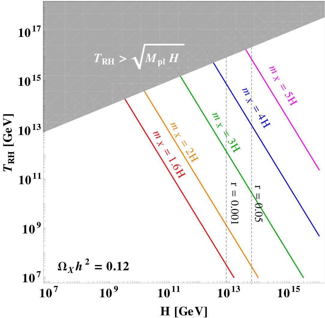 Figure 1
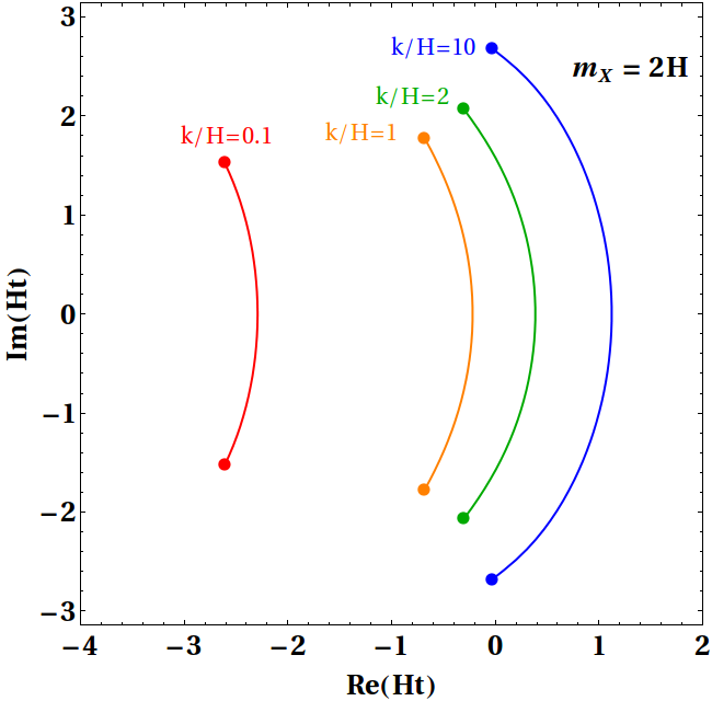 Figure 2
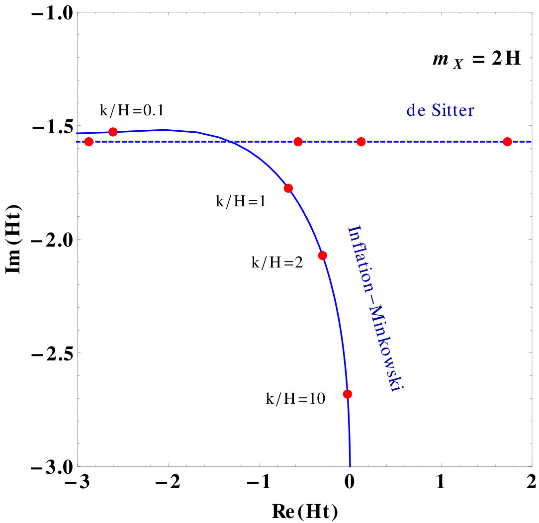 Figure 3
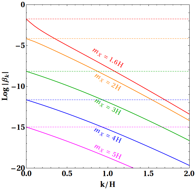 Figure 4
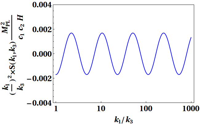 Figure 5
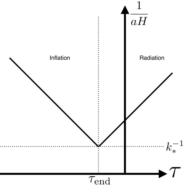 Figure 6
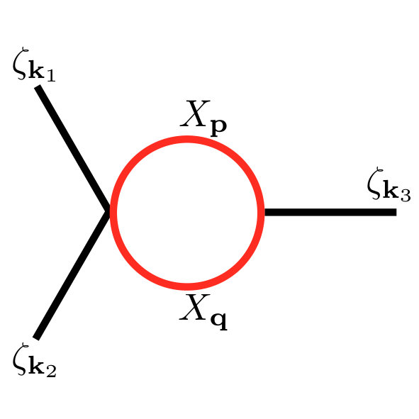 Figure 7
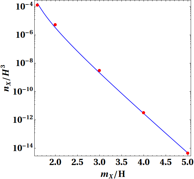 Figure 8
Peer Reviews
No public reviews on file for this paper yet. If you reviewed it on a platform where reviews are public (OpenReview, ICLR, NeurIPS, ICML), you can paste yours below so the community can read it here.
Videos
No videos yet. Explain this paper in a talk, walkthrough, or lecture? Add one.
Gravitational Production of Superheavy Dark Matter and Associated Cosmological Signatures
Lingfeng Li1, Tomohiro Nakama1, Chon Man Sou2,1, Yi Wang2,1, Siyi Zhou2,1
[email protected],[email protected],[email protected], [email protected], [email protected]
1Jockey Club Institute for Advanced Study, The Hong Kong University of Science and Technology,
Clear Water Bay, Kowloon, Hong Kong, P.R.China
2Department of Physics, The Hong Kong University of Science and Technology,
Clear Water Bay, Kowloon, Hong Kong, P.R.China
Abstract
We study the gravitational production of super-Hubble-mass dark matter in the very early universe. We first review the simplest scenario where dark matter is produced mainly during slow roll inflation. Then we move on to consider the cases where dark matter is produced during the transition period between inflation and the subsequent cosmological evolution. The limits of smooth and sudden transitions are studied, respectively. The relic abundances and the cosmological collider signals are calculated.
I Introduction
CDM cosmology has succeeded in explaining the existence and structure of the cosmic microwave background (CMB), the large-scale structure (LSS), the abundances of the light elements and the accelerating expansion of the universe. However, the nature of cold dark matter (CDM) Bertone:2004pz , including its production mechanism and interactions, is still not known.
There are many production mechanisms of dark matter, one of which is gravitational particle production Ford:1986sy . In this case, dark matter can be produced during inflation and in post-inflationary phases as well. The relevant models of dark matter include Planckian Interacting Dark Matter (PIDM) Garny:2015sjg ; Garny:2017kha ; Hashiba:2018iff ; Haro:2018zdb ; Hashiba:2018tbu , WIMPZILLA Kolb:1998ki ; Kolb:2007vd , SUPERWIMP Feng:2010gw , FIMP Hall:2009bx (the model considered in Garny:2015sjg can be viewed as “FIMPZILLA”).
In this paper, we focus on Superheavy Dark Matter (SHDM) Chung:1998zb ; Kuzmin:1998uv ; Chung:1999ve ; Kuzmin:1999zk ; Chung:2001cb , for which . The existence of such dark matter may originate from supersymmetry breaking theories Delacretaz:2016nhw , string inspired models Chang:1996rf ; Chang:1996vw ; Faraggi:1999iu ; Coriano:2001mg or Kaluza-Klein theory of extra dimension Garny:2015sjg ; Garny:2017kha ; Kumar:2018jxz . The amount of gravitational dark matter production during inflation is well known and it is roughly proportional to , where . In reality, after inflation, there will eventually be the radiation-dominated universe. There are a variety of mechanisms of the so-called preheating/reheating period sandwiched between the inflation and radiation-dominated universe Kofman:1994rk ; Kofman:1997yn (see Bassett:2005xm ; Boyanovsky:1996sv ; Allahverdi:2010xz ; Frolov:2010sz ; Amin:2014eta for reviews). When the mass of the gravitationally produced dark matter particle is large, the production rate is in general exponentially suppressed in terms of the mass of the dark matter particle. In this case, the produced superheavy dark matter particle may not be sufficient to explain the existing dark matter relic abundance. However, as noted recently in Ema:2018ucl , during an inflaton oscillation regime Ema:2015dka ; Ema:2016hlw , where the scale factor oscillates very rapidly, dark matter particles with number density proportional to can be produced. An analytical approach for this case is developed recently in Chung:2018ayg .
We discuss that there is another scenario where the number density of order superheavy dark matter can be produced, where there is a sharp transition between the inflation-radiation period. This may be realized in some inflationary models such as quintessential inflation Peebles:1998qn , as discussed later.
We will also revisit smooth transition cases by introducing the Stokes line method, which was used in the analysis of the Schwinger effect Dabrowski2014 . In the community of the gravitational dark matter production, the common method is to calculate the Bogoliubov coefficients in the WKB approximation Chung:1998bt ; Quintin:2014oea ; Celani:2016cwm which assumes that the mode functions of the fields are close to adiabatic mode functions. Quantum transitions such as excitations with slowly changing Hamiltonian Berry1990 ; Berry1993 ; Betz2004 and particle productions in slowly changing background Winitzki:2005rw are exponentially small, implying that the desired Bogoliubov coefficients can not be calculated by introducing a normal series solution with integer orders. On the other hand, the characteristics of mode functions change considerably during the universe’s expansion, and we have to identify carefully the dominant and subdominant parts in the WKB ansatz Dumlu2010 in order to interpret the Bogoliubov coefficients as particle productions. Some researchers Kim2010 ; Kim2013 ; Dumlu2010 ; Dabrowski2014 ; Dabrowski2016 considered these questions and argued that the evaluations of particle productions require more information besides WKB ansatz, i.e. the Stokes phenomenon which involves the emergence of subdominant component with negative frequency Higham2015 . These studies imply that the Stokes phenomenon can indicate the production events and provides results with a reasonable precision, and therefore we may adopt this interpretation. On the other hand, the ref. Berry1989 showed that the superadiabatic approximation can describe universal and smooth particle productions when the time evolution hits the Stokes line. This method utilizes Dingle’s theory of asymptotic series Dingle1973 . We adopt this method to calculate the gravitational dark matter production in a smoothly changing background.
There are many models for gravitationally produced dark matter with different mass ranges and different types of interactions Chung:2004nh ; Chung:2011ck ; Chung:2013rda ; Kannike:2016jfs ; Alonso-Alvarez:2018tus ; Kolb:2017jvz ; Fairbairn:2018bsw ; Garny:2018grs . One may ask if it is possible to determine some properties of such dark matter independently of the details of these models. One such possibility is to make use of the cosmological-collider signals Chen:2009we ; Chen:2009zp ; Baumann:2011nk ; Noumi:2012vr ; Arkani-Hamed:2015bza . By measuring the squeezed-limit non-Gaussianity, from the frequency of its oscillation, we can in principle read off the mass of the dark matter particle. The spin information may also be read off from the angular dependence in the squeezed limit. Note though that the frequency depends on the inflationary Hubble scale and possible non-minimal gravitational couplings as well. Also, the coupling between dark matter and the inflaton may affect the relic abundance of dark matter, or correct the mass of the dark matter particle in a significant way, as we will discuss later.
This paper is organized as follows: In Section II, we setup the model and study three scenarios of the dark matter gravitational production in the early universe. The dark matter relic abundance is also calculated. In Section III, we discuss associated cosmological collider signals which may help to determine the mass of the gravitationally produced super-heavy dark matter particle. We conclude in Section IV.
II Dark Matter and its Relic Abundance
Consider a FRW universe with the metric . We denote the dark matter field as . The action is
[TABLE]
where is the Ricci scalar, and the last term represents the non-minimal coupling.
The equation of motion for is
[TABLE]
We can write the field in terms of modes as
[TABLE]
where and are the annihilation and creation operators that satisfy the commutation relations and . We find
[TABLE]
where is the Hubble parameter here. Note that is very small in the slow-roll inflation cases and vanishes in the case of exact de Sitter space.
We will consider three scenarios of the gravitational production of superheavy dark matter. The production in an exact de Sitter phase is reviewed in Section II.1. We use the Stokes line method to estimate the particle production in a toy universe in which inflation is connected to Minkowski spacetime in Section II.2. Section II.3 is devoted to an analysis of a sudden transition between the inflation and radiation period.
II.1 Slow Roll Inflation
In this section, we review the gravitational particle production during slow roll inflation, approximated by a period of de Sitter expansion. This part is well known and recently reviewed in Markkanen:2016aes . The particle production in the presence of a background electric field is discussed in Kobayashi:2014zza .
During slow roll inflation, the scale factor is approximately , and . When inflation ends, the scale factor starts to evolve in a non-accelerated way. There are two classes of solutions to the massive field equation of motion, corresponding to “in” state and “out” state, respectively Chen:2009we ,
[TABLE]
where is the Hankel function of the first kind, and is the Bessel function.
The mode functions are related via a Bogoliubov transformation as
[TABLE]
Inserting the explicit expressions for the “in” state mode function and “out” state mode function, we obtain the following expressions for the Bogoliubov coefficients
[TABLE]
then can be evaluated as
[TABLE]
Then
[TABLE]
gives the total number of particles produced per comoving three-volume, from the past infinity to future infinity, as shown below (see also Kobayashi:2014zza ). We can focus on the time duration when is largest. By studying the maximum value of , we know that particles are produced mostly around the time
[TABLE]
Using this relation to rewrite the integral into integral, we have
[TABLE]
Then the integral in (10) can be evaluated as
[TABLE]
The production rate per unit physical four-volume can be obtained as
[TABLE]
The physical number density of particles at each moment can be evaluated as:
[TABLE]
which is constant in time. Hence, as a particular case, can be regarded as the number density at the end of inflation. Then the current DM abundance is Chung:2001cb :
[TABLE]
in the unit of GeV. Here and are the radiation energy fraction and temperature today. This shows that the relic density is exponentially sensitive to . If we further assume that reheating happens soon enough after inflation ends, by energy conservation and , we will need GeV in order to make a major component of DM. Here we assume that production during the exact de Sitter phase is dominant and determines the eventual relic density, but it may be subdominant depending on post-inflationary phases, as we will discuss below.
II.2 Inflation Connected to Minkowski Spacetime
In this section, we discuss the case where inflation is smoothly connected to Minkowski spacetime. The particle production in this scenario would approximate the particle production in more realistic scenarios where inflation is connected to a stage of the universe with much lower Hubble scale (and thus approximately Minkowski), for example, radiation-dominated universe with transition time of order .
We introduce the Stokes line method to compute the dark matter relic abundance. The method utilizes the fact that the adiabatic expansion from the WKB approximation is a factorially divergent asymptotic series which can be resummed by the Borel’s summation. Under a proper truncation of the asymptotic series, smooth particle production is obtained while the physical time is crossing the Stokes line of mode functions Berry1989 .
We parametrize our toy model of the scale factor evolution as
[TABLE]
Note that in this subsection, is the initial Hubble parameter, which is a constant and not the Hubble parameter for all times.
For , the scale factor approaches de Sitter spacetime. For , the scale factor approaches Minkowski spacetime with approaching unity. We would like to use the Stokes line method to calculate the particle production in this toy model. This study would shed some light on the particle production in the real universe. We present the main steps in the following and leave a detailed review of this method in Appendix A. Applications of this method to the inflationary universe is also given in this Appendix A.
We use to denote the complex time on lower half-plane satisfying , and can be expressed as
[TABLE]
where is the Stokes multiplier which indicates the moment when the Stokes line is hit, and is an unimportant constant phase. Thus, the Bogoliubov coefficients are
[TABLE]
We draw the trajectory of solutions for both de Sitter and our inflation-Minkowski case on the left panel of FIG. 1. We also draw some of the Stokes lines for different modes on the right panel. We then integrate Eq. (19) numerically. The results are present on the left panel of FIG. 2. The numerical results can be fitted by
[TABLE]
The equation describes estimated by numerical integration well for a wide range of , shown on the right panel of Fig. 2.
To be consistent with observations, we require
[TABLE]
In single-field slow-roll models of inflation, the initial Hubble parameter can be related to the tensor-to-scalar ratio as Enqvist:2017kzh
[TABLE]
For , we have to explain the full dark matter relic abundance. The corresponding value for is . We draw the parameter space compatible with in Figure. 3.
II.3 Sudden Transition between Inflation and Radiation Domination
In this subsection we aim at evaluating the particle production during a sudden inflation-radiation transition, with the transition time scale . Such a situation may be realized by modifying the inflaton potential for quintessential inflation Peebles:1998qn . Radiation can also be produced gravitationally, or one can also introduce coupling between the inflaton and other fields to reheat the universe Dimopoulos:2017tud ; Hashiba:2018tbu . See also Nakama:2018gll . In this case, we can parametrize the evolution history of the universe in the following way,
[TABLE]
such that and are continuous. Note that in this subsection, is a constant parameter (initial Hubble parameter in the inflation stage), which is no longer interpreted as the Hubble parameter after the sudden transition.
The dark matter is quantized as
[TABLE]
Let us focus on subhorizon modes with , for which the mass term can be neglected. We also assume for simplicity. The mode function satisfies the Mukhanov-Sasaki equation
[TABLE]
For the modes with , the solutions can be approximated as follows. First, the above equation is solved by
[TABLE]
the coefficients can be determined by the connecting conditions and as follows:
[TABLE]
From these we find
[TABLE]
Inserting the expression of and into the expression for when ,
[TABLE]
On the other hand, the mode function can be written as
[TABLE]
where is the positive-frequency component of the mode function with the normalization condition
[TABLE]
So the Bogoliubov coefficients are given by
[TABLE]
which satisfies the normalization condition .
We have to ensure that the produced particle does not have much backreaction on our background described by Eq. (23) and (24). So we can estimate the minimum of by requiring that the energy density of the produced particles is comparable to the inflationary vacuum energy as follows:
[TABLE]
That is, as long as , backreaction is negligible. Now we estimate the particle number produced in this comoving ranging from to as
[TABLE]
Assuming , for . No matter what value of we take, the de Sitter particle production is much less than the particle production from a sudden inflation-radiation transition era. The corresponding DM relic abundance can be estimated similarly:
[TABLE]
For instantaneous reheating case, we need GeV to produce enough DM, which is much smaller compared to the ones in smooth transition scenarios as expected.
III Dark Matter on the Cosmological Collider
Let us consider an effective field theory where the dark matter sector couples to the primordial curvature perturbation in the following way An:2018tcq :
[TABLE]
These two operators can be regarded as coming from the effective field theory of inflation, or two terms coming from the full Lagrangian of the original quasi-single field inflation with a constant turning trajectory Chen:2009zp . Since if we consider other types of interactions, the procedure of obtaining the characteristic signals will be similar. Thus, we focus on these two terms for simplicity.
Due to the above interactions, the DM leaves its imprints in the primordial non-Gaussianity. Here let us assume that . The dominant contribution to the non-Gaussianity is from integrating out the dark matter field Chen:2012ge ; Pi:2012gf ; Tong:2017iat ; Iyer:2017qzw ; Wu:2018lmx . The resulting non-Gaussianity is of the shape of general single field inflation Chen:2006nt and of equilateral shape. The magnitude of non-Gaussianity is power-law suppressed in the large-mass limit Gong:2013sma .
There is another type of signal, which, in magnitude, is smaller than the equilateral shape non-Gaussianity from integrating out heavy fields. Usually they are subject to Boltzmann suppression in the large mass limit. This signal, however, is more informative and can tell us directly the mass of the dark matter field in terms of Hubble rate during inflation. This is the cosmological collider signal in the squeezed limit non-Gaussianity from which we can also measure the spin of the dark matter particle. This mechanism is known as the cosmological collider Arkani-Hamed:2015bza and is closely related to quasi-single field inflation Chen:2009we ; Chen:2009zp ; Baumann:2011nk and the primordial quantum standard clocks Chen:2015lza ; Chen:2016cbe ; Chen:2016qce .
Given the form of interactions, the (the prime indicates that we ignore the momentum-conservation factor ) is contributed by the loop diagrams. The dark matter loop can be attached to any of the , and legs. In the squeezed limit , the leading contribution to the cosmological collider signal comes from the Feynman diagram depicted in FIG. 5. The technique of computing this type of loop diagram is initially proposed in Arkani-Hamed:2015bza . The application to the Standard model mass spectrum can be found in Chen:2016nrs ; Chen:2016uwp ; Chen:2016hrz ; Wu:2017lnh , and it had also been applied to complex scalar fields in Chua:2018dqh . The crucial point is that although in general, loop diagrams may suffer from UV or IR divergence Weinberg:2010wq , and usually we need to introduce local counter terms to cancel the UV divergence, the clock-signal part of the contribution does not suffer from UV or IR divergence. The reason is that the contribution is coming from the non-local process. In this case, we only have to use a double Fourier transformation to deal with the momentum integral. We present the details of the computation in Appendix B.
It gives the standard cosmological collider signal in the squeezed limit as
[TABLE]
where the factor is
[TABLE]
We can express the bispectrum in terms of the dimensionless shape function Chen:2018xck as
[TABLE]
where is the power spectrum of the curvature perturbation without the correction caused by massive fields. We are particularly interested in the squeezed limit where . In this limit, the shape function is
[TABLE]
and we plot in FIG. 6.
The estimator of non-Gaussianity can be defined as Chen:2016hrz
[TABLE]
The modest lower bound of can be estimated for an effective field theory with Planck scale cutoff. For such a theory, and (note that a factor emerges when we canonically normalize ). This will lead to vanishingly small non-Gaussianities. For the toy universe of smooth transition, the typical value for is for , GeV and . For , GeV and , . For the instantaneous case, the typical value for is for the parameters we considered in the last section.
For the effective field theories which are not Planck mass suppressed, can be larger than , can be larger than . But too large couplings with the inflaton may change the relic abundance. To estimate the upper bound, and thus cause inconsistencies for the dark matter production.
Note that the two operators in (36) actually originates from the following two actions
[TABLE]
where and , and are related via
[TABLE]
Now we want to consider and as order one constants. The bound on the scale of the EFT should be given by the constraint that there are no overproduction of the dark matter relic abundance. Note that the decay chanel from a single inflaton to dark matter is kinematically forbidden since the inflaton is lighter than the dark matter. Thus, to check the relic abundance, the leading contribution comes from the dark matter produced by collisions of the thermalized inflaton particles.
The explicit form of the constraint depends on the details of reheating. If the inflaton is thermalized rather efficiently during reheating, to get the correct relic abundance for dark matter, we need
[TABLE]
For the typical parameter space, we have . Depending on the reheating temperature, can take different values.
On the other hand, if the inflaton has no chance to be thermalized, the above bound does not apply. For example, one may consider brane inflation for the sudden transition Dvali:1998pa ; HenryTye:2006uv , where the inflaton just disappears at the moment of reheating. In addition, for smooth transition, one may consider quintessential inflation, where reheating can also be realized by gravitational particle production, without assuming the coupling between the inflaton and the standard model sector. In principle, dark matter can be created from the inflaton during kination as well, but during kination the energy density of the inflaton gets redshifted rapidly , and hence this production would not cause a problem for our estimations. One can also consider a scenario where the inflaton decays to a heavy field, while dark matter is created gravitationally at the end of inflation, and the former heavy field may later decay to radiation to reheat the Universe. In this case the reheating temperature is determined by the decay rate of the heavy field, and then the reheating temperature can be chosen to be sufficiently low so that dark matter cannot get produced at the reheating. In general, either way, we need to discuss gravitational particle production by a smooth transition from inflation to kination or an early matter domination, and applying the Stokes line method to such situations would also be possible, though we used a smooth transition from inflation to Minkowski spacetime for simplicity. In gravitational reheating one also needs to worry about an overproduction of gravitons, but this issue can be circumvented by spinodal instability of the Higgs or by introducing a sufficient number of degrees of freedom for radiation gravitationally produced Nakama:2018gll . One can also use a scenario of Hashiba:2018tbu . We estimated the relic abundance assuming smooth transition from inflation to radiation domination, but an extension of that analysis to cases with a kination phase inserted would be straightforward.
Another lower bound on (and thus upper limit on ) can be obtained from the consideration that (42) does not change the dark matter mass too much (otherwise we lose the prediction power for the mass of the dark matter particle on the cosmological collider). For instance, if and this means if , then this additional term is negligible. Otherwise, the mass of dark matter on the cosmological collider will significantly differ from the probes that we expect to use to observe dark matter now. This limit will generically give . Thus, we expect that if the cosmological collider signal is observed for such dark matter production scenarios, it is very likely that the observed mass of the dark matter is strongly corrected by the inflaton coupling. However, this conclusion depends on the coupling details between the inflaton and the dark matter. Since we haven’t exhausted all possible couplings between the inflaton and dark matter, rather only studied the simplest ones, it remains interesting to see if there can be dark matter couplings with the inflaton which can naturally take large values.
The dark matter field may also leave some imprints on the power spectrum through the relation which relates and when the comoving momentum of is soft Chung:2013sla . However, these relations may not show characteristic features of dark matter, but rather are universal for all matter components Pajer:2013ana . For example, one can expand the correlation function in the series of the ratio between the soft leg and the hard leg. The leading order gives the Maldacena consistency relation which is fixed by dilatation symmetry Maldacena:2002vr . The next-to-leading order is fixed by special conformal symmetry Creminelli:2004yq . It is thus unclear how to extract dark mater properties from these correlators.
Finally, we briefly comment possible isocurvature fluctuations from dark matter. A field like that is not directly coupled to the inflaton will introduce isocurvature perturbation. From ref. Chung:2004nh , we can estimate the size of as
[TABLE]
Since is a heavy field ( 0), , which has no significant dependence. At large scale, , will be suppressed by . In other words, the power of isocurvature mode is diluted by inflation with e-folds. Therefore we do not expect any large scale isocurvature signal to be observed.
IV Conclusion
We considered three cosmological scenarios and calculated the dark matter relic abundance produced gravitationally. Our conclusions are as follows: For exact de Sitter space, the number density is proportional to , where . For a universe where inflation is connected to a Minkowski universe, we used the Stokes line method to calculate the dark matter relic abundance. The resulting number density is exponentially suppressed. We fit the results numerically by Eq. (20). For a sudden transition where inflation is immediately connected to a radiation-dominated universe, the produced particle number density is proportional to .
The cosmological collider signal of the dark matter particle is discussed. We note that with the simplest couplings between the inflaton and dark matter, for the inflaton coupling to satisfy two conditions: (1) does not overproduce dark matter and (2) does not correct the dark matter mass significantly, the non-Gaussianity produced is too small to observe in future observations. It is interesting to see if there are mechanisms to boost the non-Gaussianity of the scenario to observational range to test the scenarios of gravitationally produced superheavy dark matter.
Acknowledgments
We thank Xingang Chen, Yohei Ema and Zhong-Zhi Xianyu for useful discussions on general mechanisms for gravitational particle production. This work is supported in part by ECS Grant 26300316 and GRF Grant 16301917 and 16304418 from the Research Grants Council of Hong Kong.
Appendix A Particle Production from the Divergent Asymptotic Series Method
In this appendix, we review the divergence series method and use it to study the particle production for general FRW backgrounds. We will first summarize the result in A.1. The summarized result will then be derived in A.2. In A.3, as a simple example, we use this method to recover the known results for particle production in de Sitter space.
A.1 Summary of the Result
To study the particle production problem, we start from the equation of motion of the massive field, which can be rewritten as
[TABLE]
This equation, together with the instant Minkowski initial condition, defines the problem of particle production on FRW backgrounds.
As inspired by scattering problems in quantum mechanics, the sign of determines whether the mode function is oscillating or decaying in a “potential barrier”, and the moments when are turning points. For large enough mass , the turning points can be complex. The phase integral along a particular complex line crossing the real axis is connected to an exponentially small component in the mode function Berry1989 .
We denote as the complex time located at lower half-plane which makes , together with a phase accumulated from
[TABLE]
The contour to carry out the integral will be specified in Eq. (51).
We define the Dingle’s singulant variable
[TABLE]
With these definitions, we write down the form of the approximate solution of Eq. (46) Berry1989 :
[TABLE]
where is called the Stokes multiplier function
[TABLE]
The constant factor in the first line of Eq. (49) is for matching the adiabatic vacuum when , and the amplitude of the negative-frequency part is then suppressed by the exponential
[TABLE]
The moment when corresponds to the emergence of the negative-frequency part of the mode function, and the set of complex satisfying this condition forms the Stokes line Berry1989 . In the above equation, is where the Stokes line intersects the real time axis. In the integration, we first integrate from to along the Stoke line, then integrate from to t along the real axis.
From Eq. (49), the approximated Bogoliubov coefficients can be extracted as
[TABLE]
which agrees with the results shown in Dumlu2010 ; Dabrowski2014 ; Dabrowski2016 .
A.2 The Divergent Asymptotic Series Method
As suggested by Dingle Dingle1973 and Berry Berry1989 , to get the particle production in (49), we assume that the dominant part of Eq. (46) has an asymptotic series solution in terms of a large parameter (or using in the cases with constant ).
[TABLE]
where is the -th order correction. Substitute the series in Eq. (46), yielding
[TABLE]
It is convenient to introduce a variable to investigate the analytic property of the differential equation. With this substitution, Eq. (54) becomes
[TABLE]
By rearranging the equation and integration by part, Eq. (55) generates
[TABLE]
Using the fact that corresponds to and matching the orders of in the series (53), we obtain a recurrence relation for :
[TABLE]
Since the series is expanded around , it is reasonable to investigate the recurrence relation around this point. Assuming that is analytical around , we can expand in terms of :
[TABLE]
By defining a variable
[TABLE]
Eq. (57) reduces to a polynomial differential equation
[TABLE]
where we keep only the dominant term in the integrand. This recurrence relation can be solved by applying an ansatz
[TABLE]
Let , the approximation for near is then given by
[TABLE]
This solution is quite complicated, but it is enough to know the divergent behavior when . We rewrite Eq. (62) in terms of the singulant variable in the large- limit as
[TABLE]
One can easily check that which agrees with the ansatz of asymptotic series (53), and this equation indicates that the series is divergent in factorial form. We will show that the factorial divergence is crucial since it is related to the Borel summation which generates a subdominant term in the solution.
Now we apply Berry’s theory Berry1989 to derive the Stokes multiplier function shown in Eq. (50) which describes the moment when massive particles emerge. To handle a divergent asymptotic series such as Eq. (53), the standard method Higham2015 is to truncate the series into a finite sum and a divergent tail as
[TABLE]
assuming is large enough so that Eq. (63) is applicable. By comparing with Eq. (49), the terms inside the square bracket is the Stokes multiplier, and we then apply the Borel summation to make the series sum meaningful. The first step is to convert the factorial into the integral of Gamma function, and we denote the multiplier as
[TABLE]
where the variable changes to in the last line, and the contour is deformed that the upper limit is . The denominator indicates that the magnitude of the integrand dominates at , and we can choose such that the phase is stationary at , implying that the integral can be evaluated with saddle-point approximation. Before proceeding the calculation of , we first justify two conditions required by the validity of the saddle-point approximation: has to be sufficiently close to since adjusting can only cancel the real part of the exponent, and has to be large enough such that Eq. (63) is applicable. The first condition is valid when the evolution is close to the Stokes line when , implying that the saddle point approximation is valid around the particle production, and it is sufficient to explain the emergence of the sub-dominant term in the mode function. To justify the second condition, we use the fact that is a constant on real axis and proportional to the large parameter . For the cases we considered in this paper, is sufficiently large as long as .
With the notations and , we expand the integrand in Eq. (65) around and approximate the integral from to :
[TABLE]
where the constant
[TABLE]
and we apply the fact in the last line that as long as is sufficiently large. Physically, the initial condition requires when is small, which indicates that the correct should be . In the original method Berry1989 this is handled by taking the principal value of the integral. Here we show that one can also evaluate by deforming the contour near the origin to be an infinitesimally small semicircle below the singularity . Since the integrand is odd, only the integral over the semicircular contour contributes to Wong1990 :
[TABLE]
Thus indeed satisfies the initial condition when is small and . Moreover, Eq. (66) also indicates that the particle productions of massive fields are governed by the error function, and the moment of productions is represented by the time which satisfies .
A.3 Example: Particle Production in de Sitter
We now show that Eq. (52) does provide us a reasonable estimation of the Bogoliubov coefficients in inflation scenario . For the massive field theory with , Eq. (46) becomes
[TABLE]
where , and the complex solutions which are closest to real axis are given by
[TABLE]
Given the exact phase integral
[TABLE]
we can derive in the inflation scenario
[TABLE]
which agrees with the definition of de Sitter temperature, and the Stokes multiplier is
[TABLE]
For the mode with smaller , it leaves horizon earlier. This is indicated by larger value of which makes the first term in the error function of Eq. (73) dominates. The numerical solution of the zero imaginary part of Eq. (71) shows that the typical production time of each mode satisfies the relation
[TABLE]
Appendix B Details of the Computation of the Loop Diagram
In this section, we present the details of the derivation of the cosmological collider signal of (37). We used the Schwinger-Keldysh formalism Chen:2017ryl . Alternatively, one can use the in-in formalism Weinberg:2005vy ; Chen:2010xka ; Wang:2013eqj .
The quantization of the field takes the form
[TABLE]
Then is related to as
[TABLE]
The second order action for the primordial curvature perturbation is
[TABLE]
where is the slow-roll parameter. Quantizing it in the following way
[TABLE]
where , are the creation and annihilation operators satisfying the usual commutation relations:
[TABLE]
The mode function satisfies the following equation of motion
[TABLE]
To the lowest order in slow-roll parameter, the solution is
[TABLE]
In order to calculate the cosmological collider signal of primordial bispectrum analytically, we first simplify the propagators for , , , , and , as
[TABLE]
where denotes the Heaviside step function. We can analogously define four types of propagators for , , , , in terms of .
We rewrite the terms in Eq. (81) to (84) in terms of the Bogoliubov coefficients defined in Eq. (7):
[TABLE]
from which we know that only the terms with and are different. However, the and terms are local, thus do not contribute to the cosmological collider signal Arkani-Hamed:2015bza ; Lee:2016vti . In order to understand the bispectrum in the squeeze limit, we focus on the terms proportional to and , then the four types of propagators , , and become identical.
[TABLE]
The squeezed-limit bispectrum can be calculated for all orders in the expansion with . Hereafter, we assume is real. The massive scalar propagators become
[TABLE]
However, for simplicity, we focus on the first order in expansion, where the Bessel J function is expanded as
[TABLE]
Then the propagator becomes
[TABLE]
Noting that
[TABLE]
and we obtain
[TABLE]
and also
[TABLE]
On the other hand, the bispectrum is expressed as
[TABLE]
Since and are constrained by momentum conservation ,
[TABLE]
First we write the delta function into an integration of exponential function in space and integrate out and by Fourier transform. To write this procedure more explicitly, we have
[TABLE]
and the Fourier transform is given by
[TABLE]
Then, we integrate out . After this procedure, we obtain
[TABLE]
where we have used the fact that . Finally, we obtain the non-Gaussianity as
[TABLE]
where the factor is given by
[TABLE]
The reference list from the paper itself. Each links out to its DOI / PubMed record.
- 1(1) G. Bertone, D. Hooper and J. Silk, “Particle dark matter: Evidence, candidates and constraints,” Phys. Rept. 405 , 279 (2005) [hep-ph/0404175].
- 2(2) L. H. Ford, “Gravitational Particle Creation and Inflation,” Phys. Rev. D 35 , 2955 (1987).
- 3(3) M. Garny, M. Sandora and M. S. Sloth, “Planckian Interacting Massive Particles as Dark Matter,” Phys. Rev. Lett. 116 , no. 10, 101302 (2016) [ar Xiv:1511.03278 [hep-ph]].
- 4(4) M. Garny, A. Palessandro, M. Sandora and M. S. Sloth, “Theory and Phenomenology of Planckian Interacting Massive Particles as Dark Matter,” JCAP 1802 , no. 02, 027 (2018) [ar Xiv:1709.09688 [hep-ph]].
- 5(5) S. Hashiba and J. Yokoyama, “Gravitational reheating through conformally coupled superheavy scalar particles,” JCAP 1901 , no. 01, 028 (2019) [ar Xiv:1809.05410 [gr-qc]].
- 6(6) J. Haro, W. Yang and S. Pan, “Reheating in quintessential inflation via gravitational production of heavy massive particles: A detailed analysis,” JCAP 01, 023 (2019) [ar Xiv:1811.07371 [gr-qc]].
- 7(7) S. Hashiba and J. Yokoyama, “Gravitational particle creation for dark matter and reheating,” ar Xiv:1812.10032 [hep-ph].
- 8(8) E. W. Kolb, D. J. H. Chung and A. Riotto, “WIM Pzillas!,” AIP Conf. Proc. 484 , no. 1, 91 (1999) [hep-ph/9810361].