3D non-LTE line formation of neutral carbon in the Sun
A. M. Amarsi, P. S. Barklem, R. Collet, N. Grevesse, M. Asplund

TL;DR
This paper develops a 3D non-LTE model for neutral carbon line formation in the Sun, providing more accurate abundance measurements and a new approach to modeling hydrogen collisions.
Contribution
It introduces a physically-motivated recipe for hydrogen impact excitation rates in non-LTE models and applies it to derive the first fully consistent 3D non-LTE solar carbon abundance.
Findings
Non-LTE abundance corrections reach up to 0.1 dex.
The derived solar carbon abundance is log ε_C = 8.44 ± 0.02.
Models reproduce observed center-to-limb variations without adjusting collision rates.
Abstract
Carbon abundances in late-type stars are important in a variety of astrophysical contexts. However C i lines, one of the main abundance diagnostics, are sensitive to departures from local thermodynamic equilibrium (LTE). We present a model atom for non-LTE analyses of C i lines, that uses a new, physically-motivated recipe for the rates of neutral hydrogen impact excitation. We analyse C i lines in the solar spectrum, employing a three-dimensional (3D) hydrodynamic model solar atmosphere and 3D non-LTE radiative transfer. We find negative non-LTE abundance corrections for C i lines in the solar photosphere, in accordance with previous studies, reaching up to around 0.1 dex in the disk-integrated flux. We also present the first fully consistent 3D non-LTE solar carbon abundance determination: we infer log = , in good agreement with the current standard…
Click any figure to enlarge with its caption.
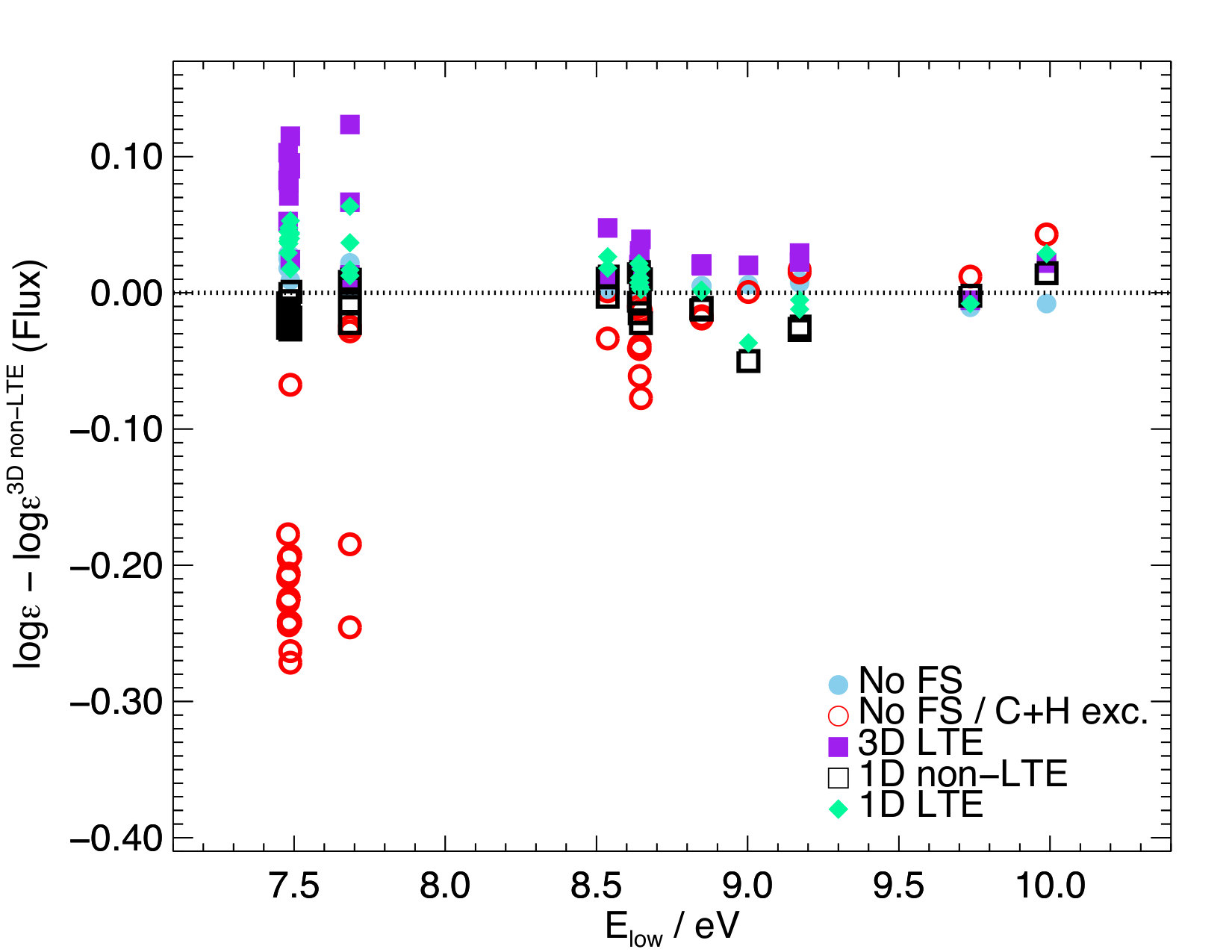 Figure 1
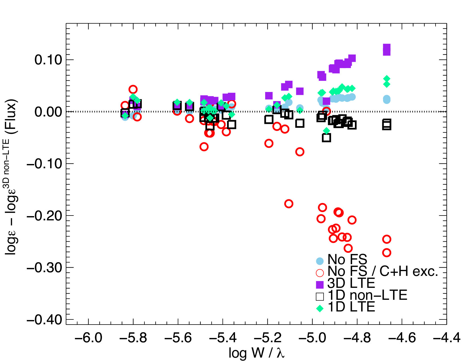 Figure 2
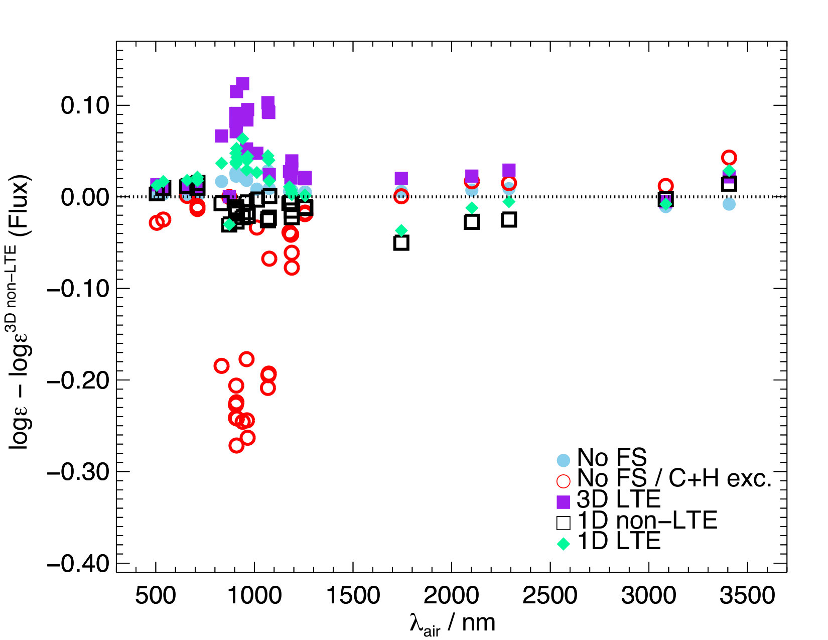 Figure 3
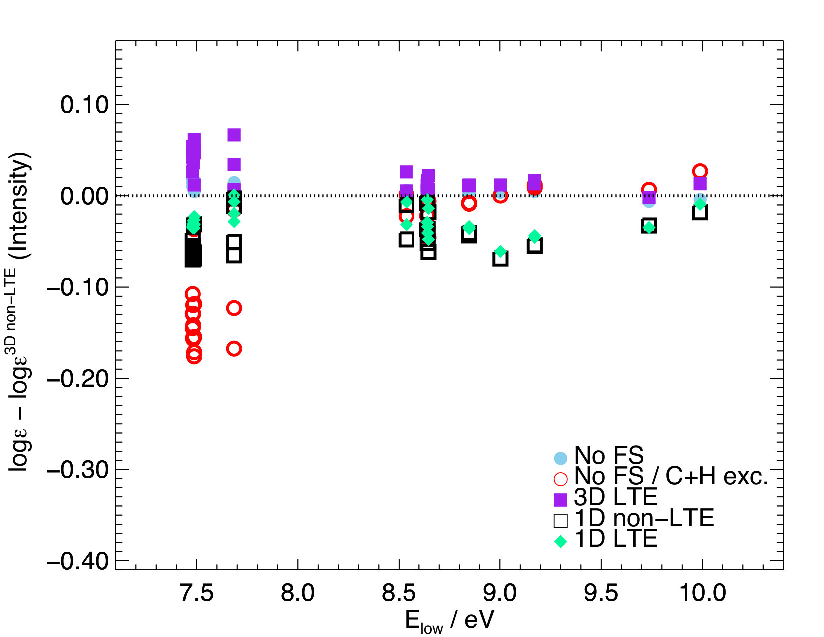 Figure 4
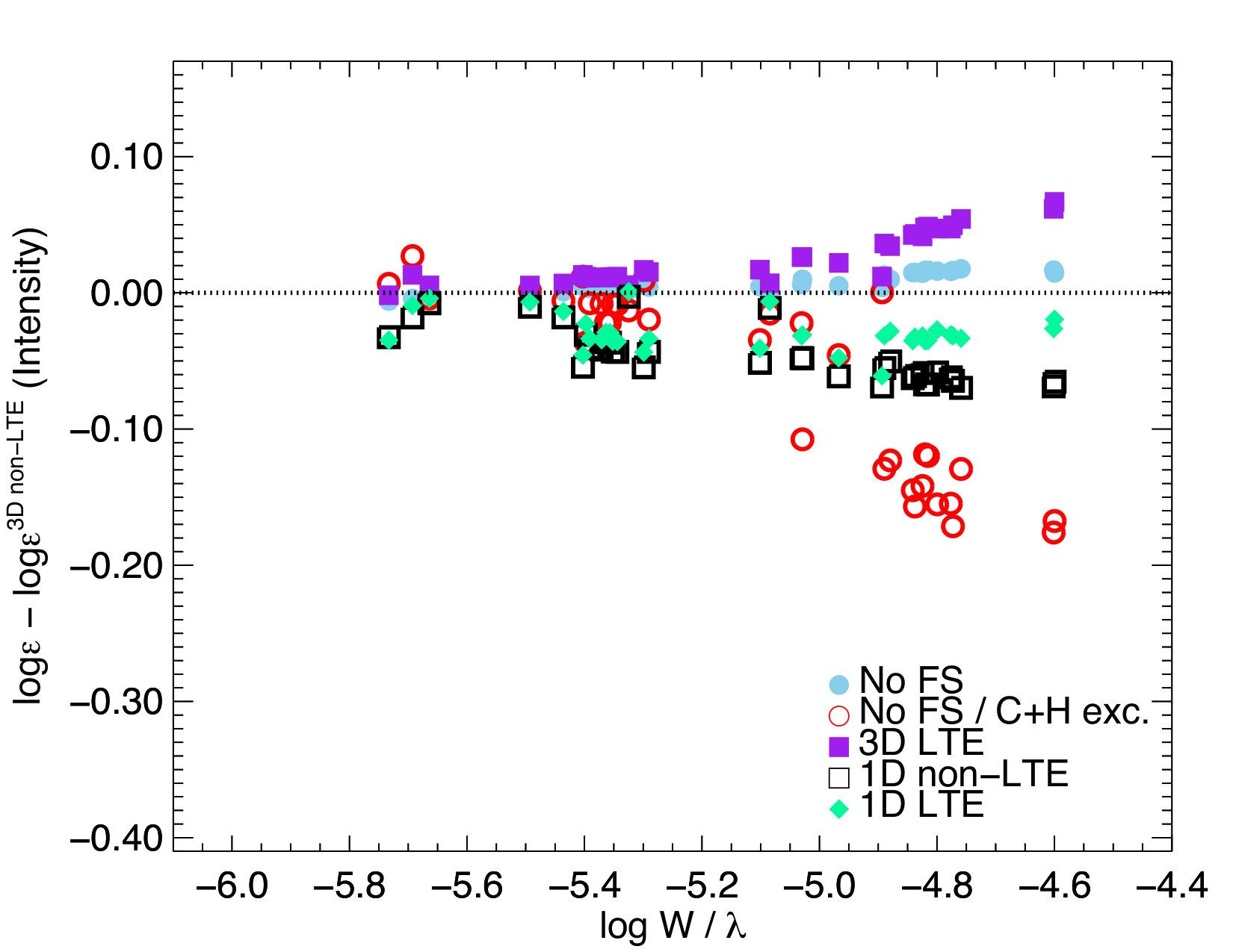 Figure 5
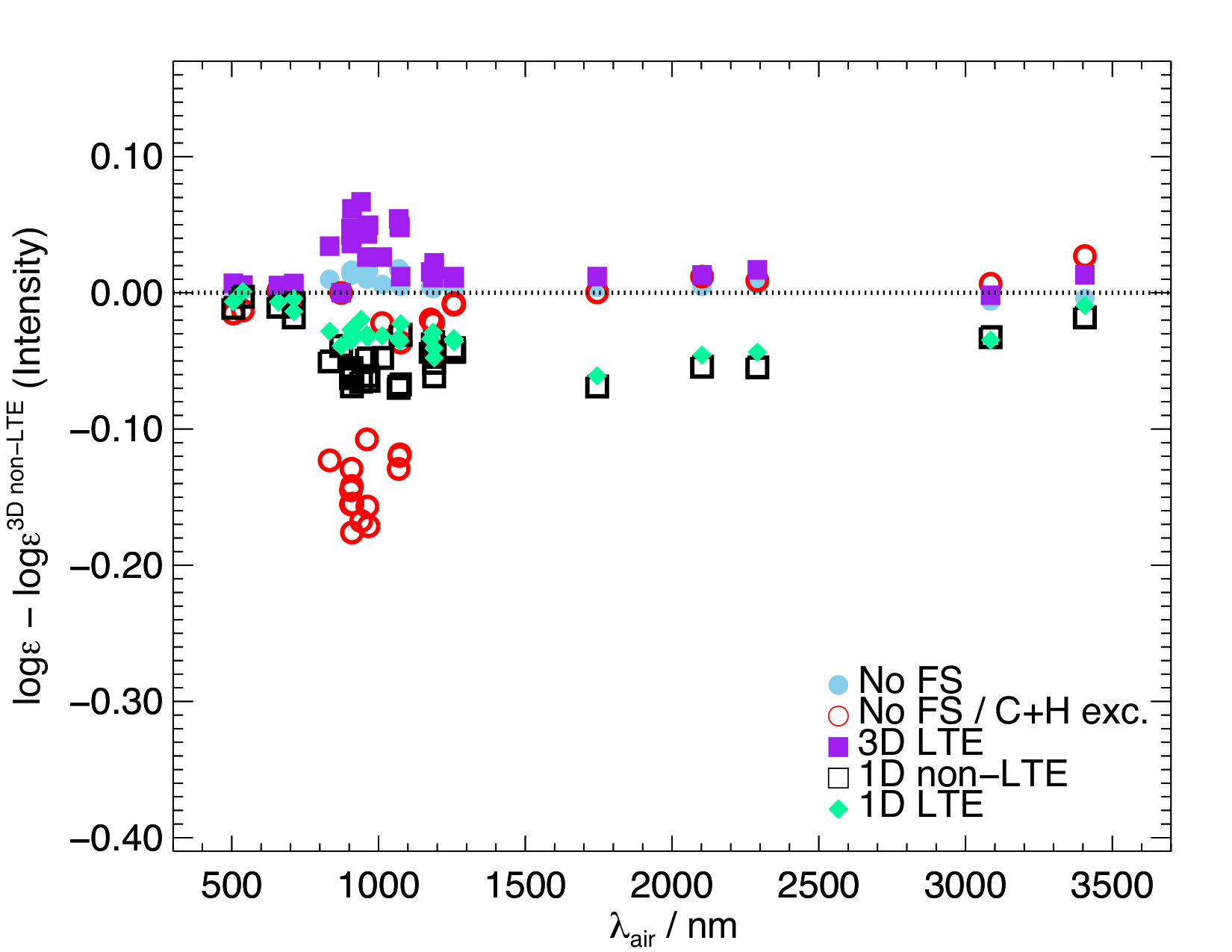 Figure 6
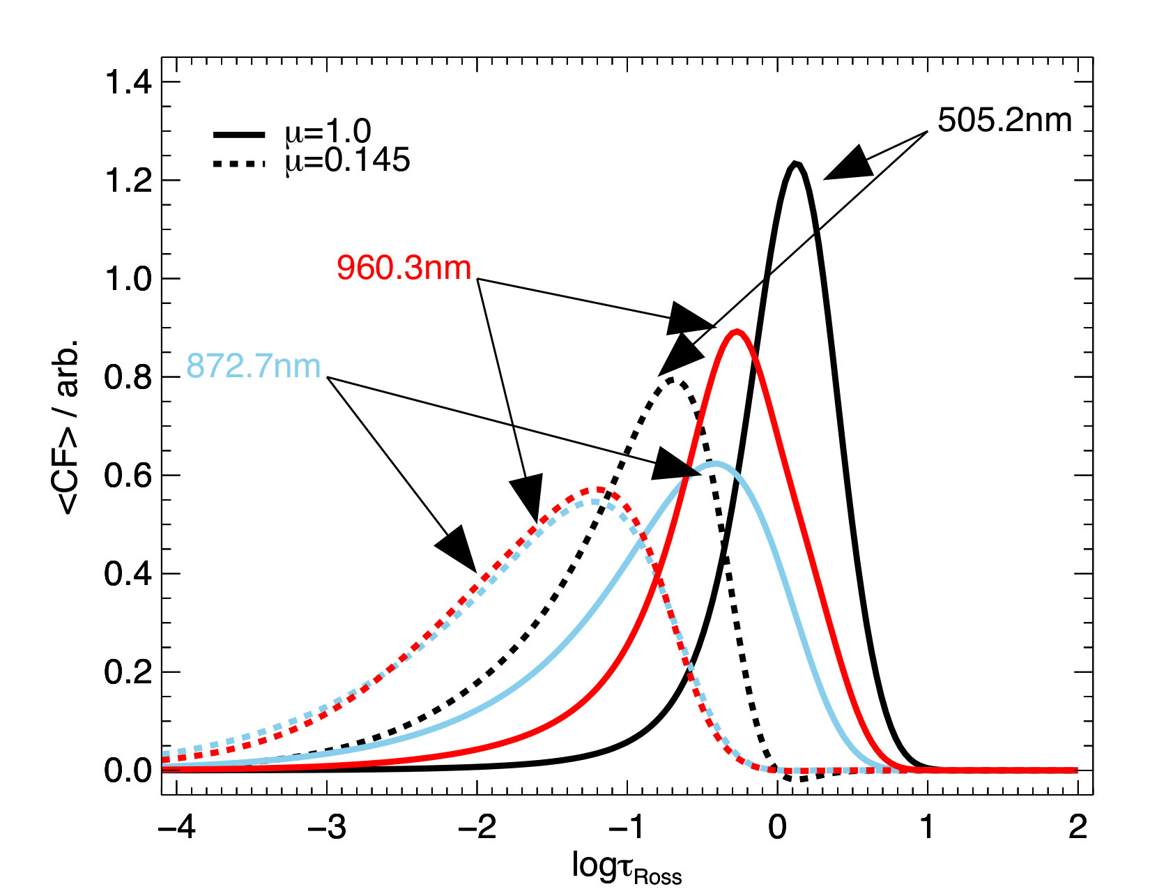 Figure 7
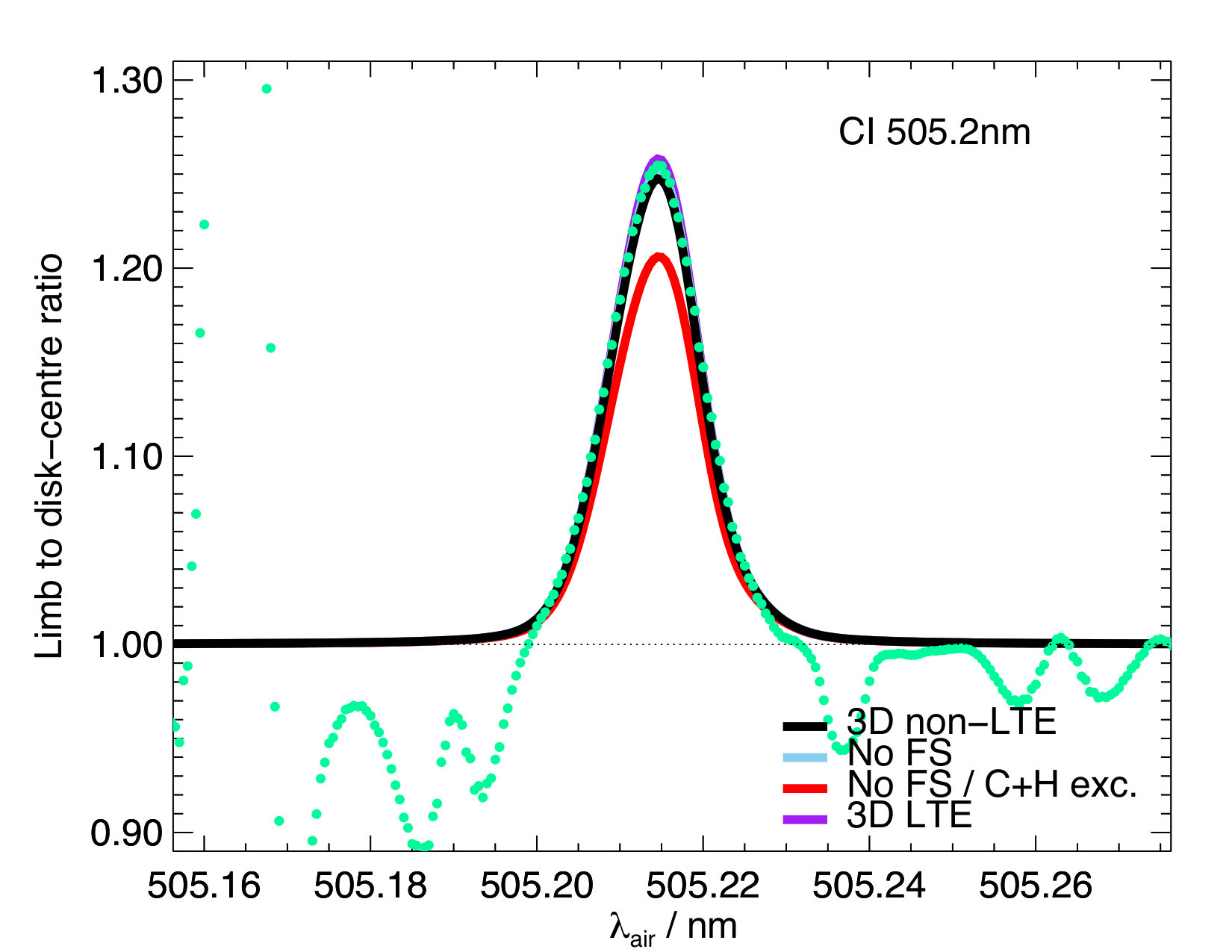 Figure 8
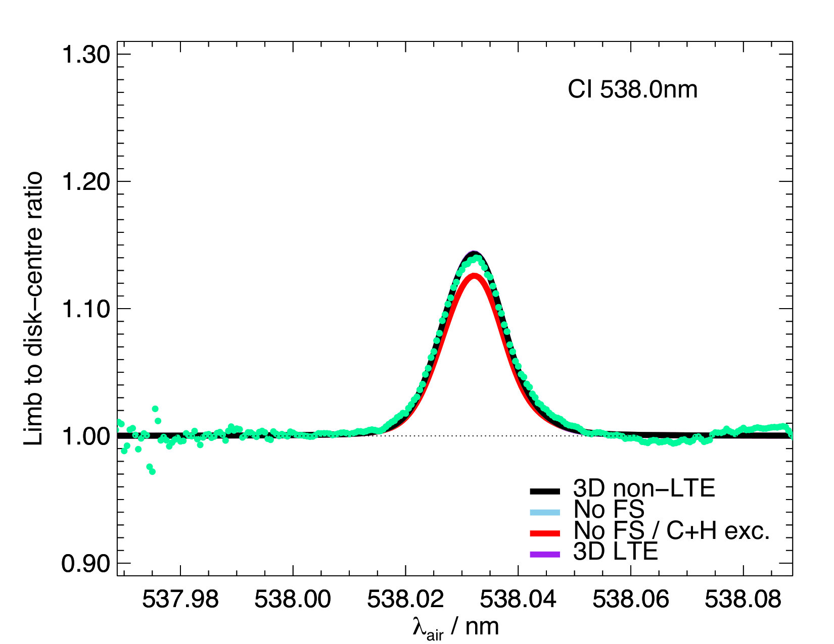 Figure 9
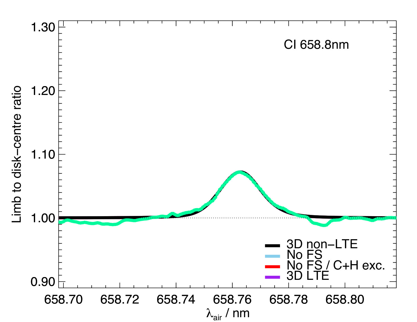 Figure 10
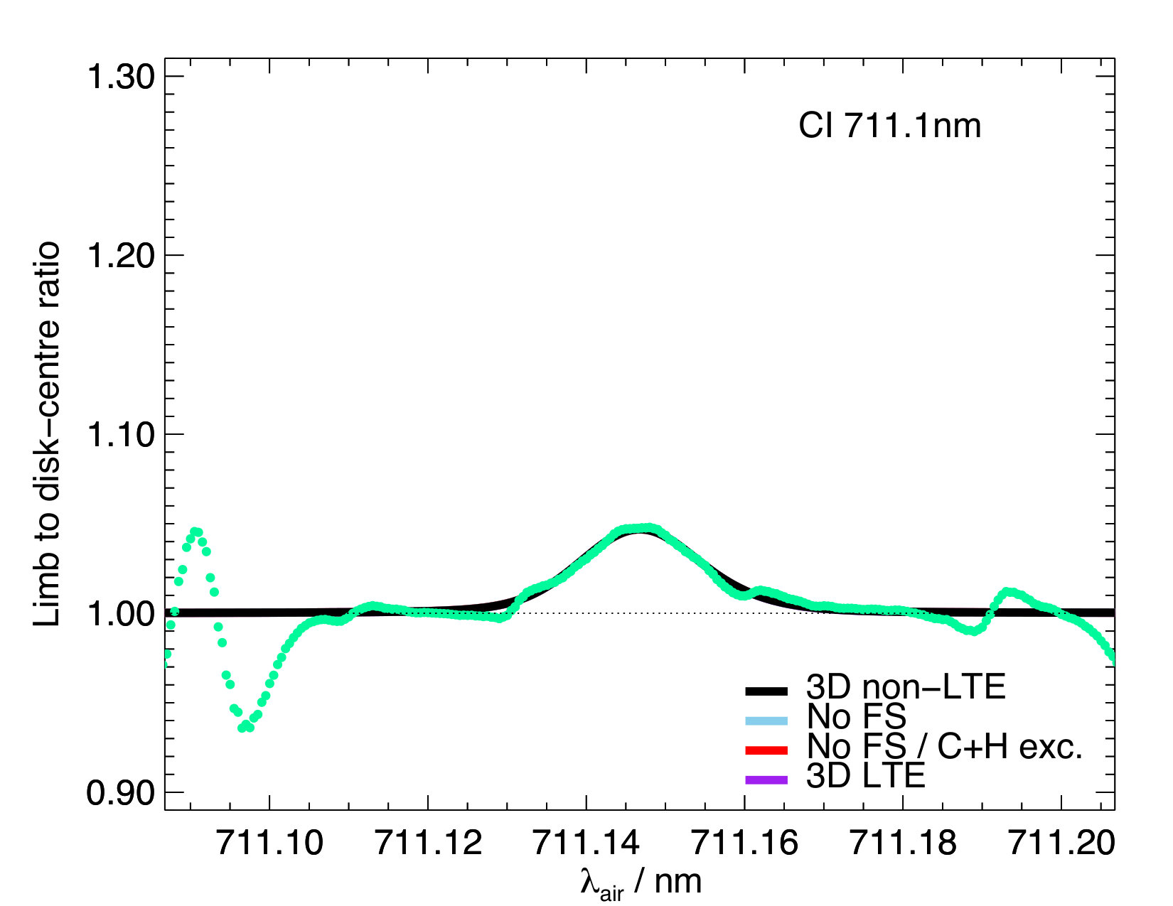 Figure 11
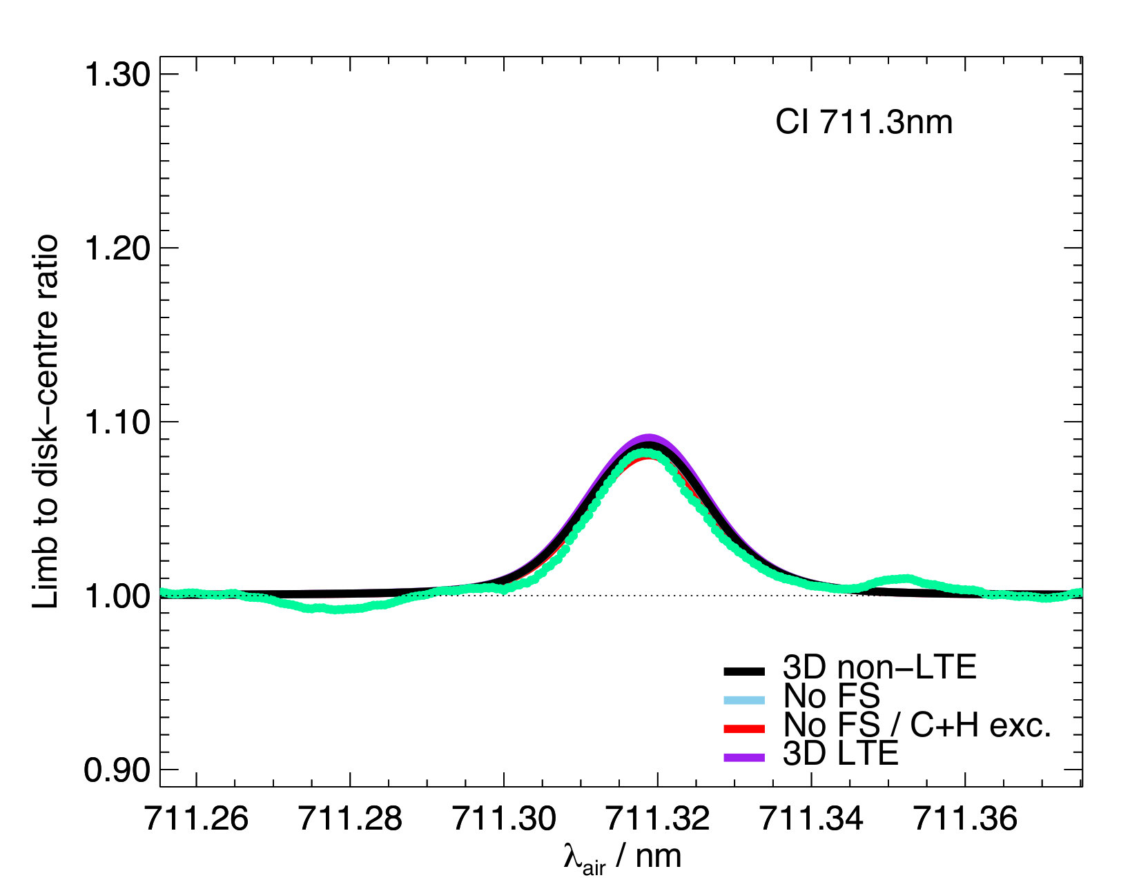 Figure 12
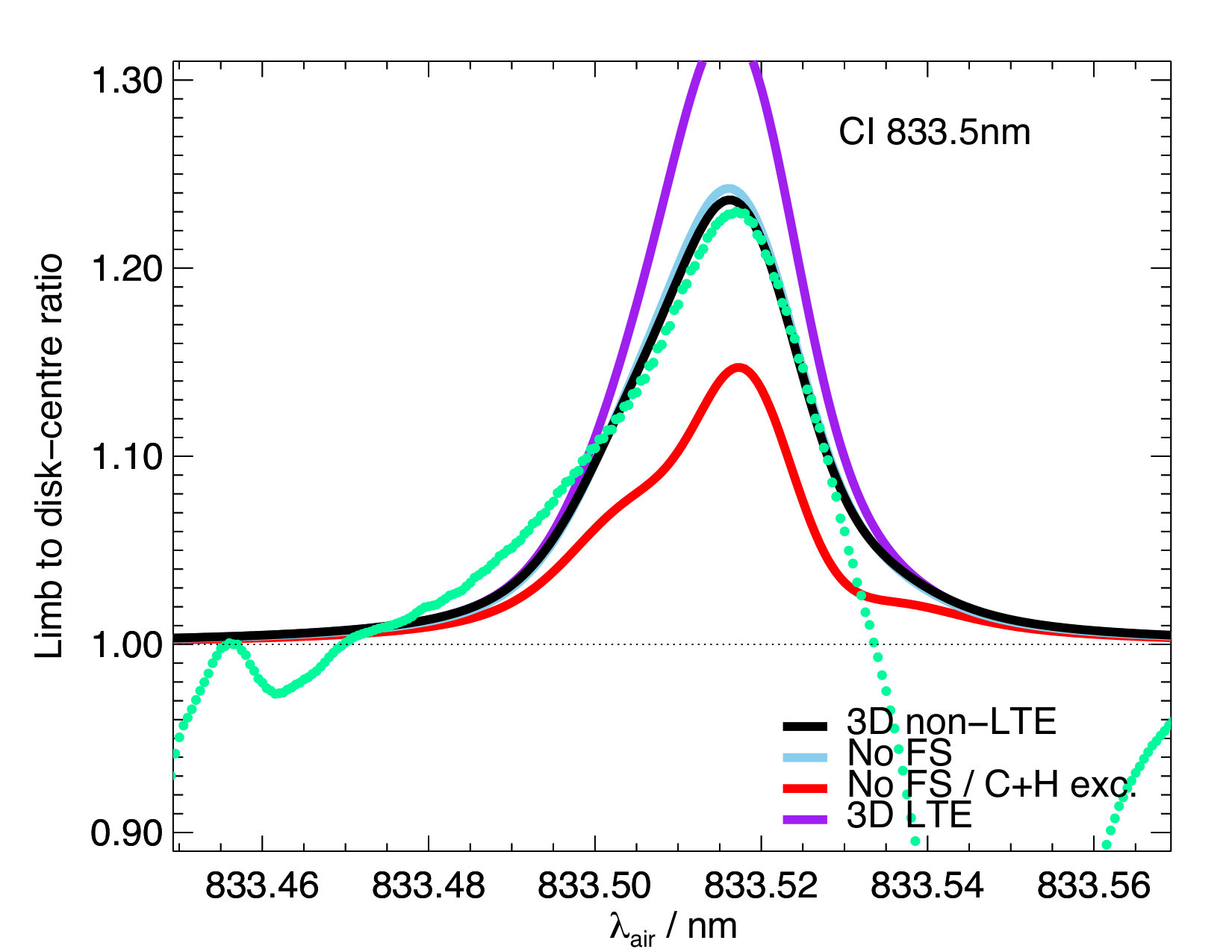 Figure 13
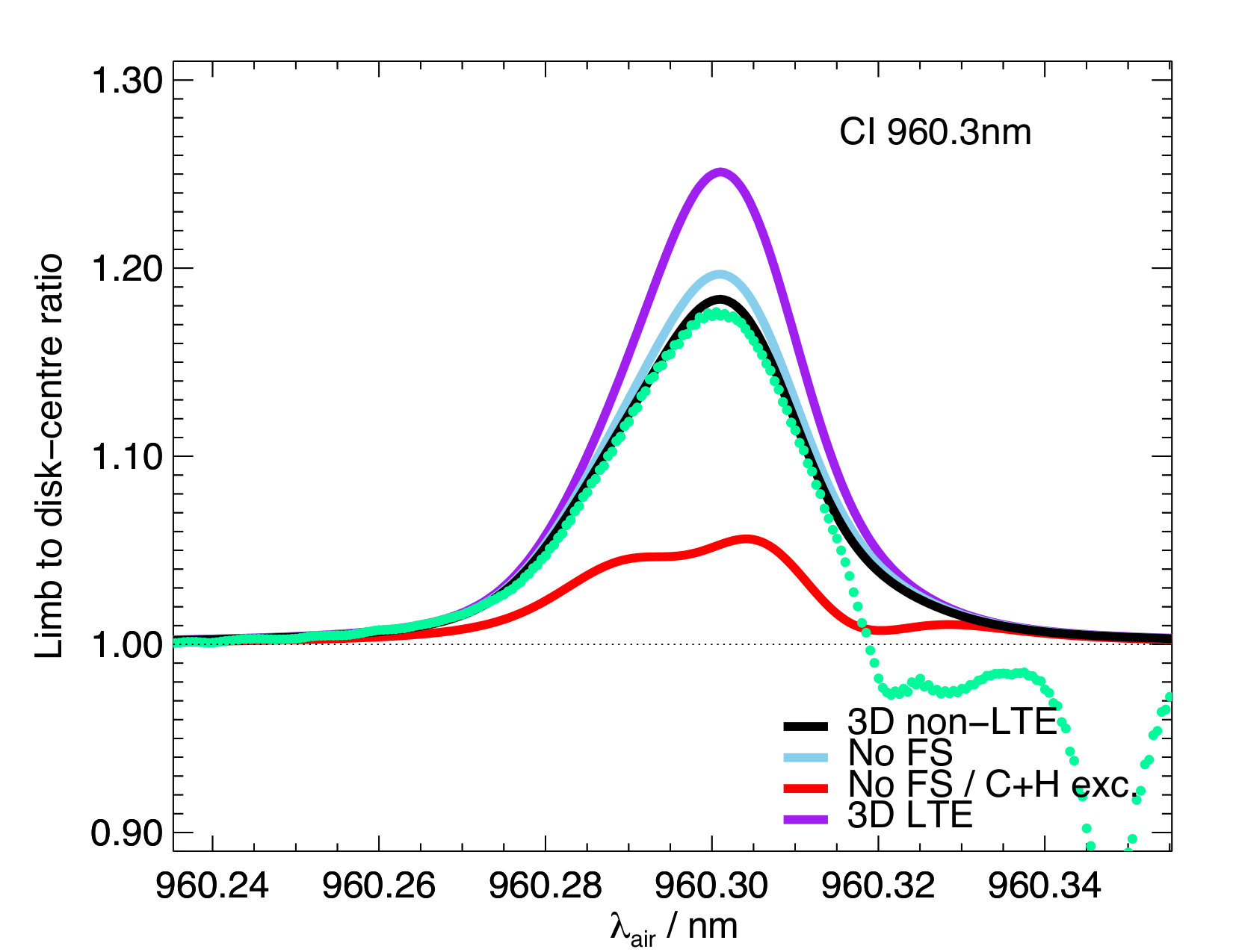 Figure 14
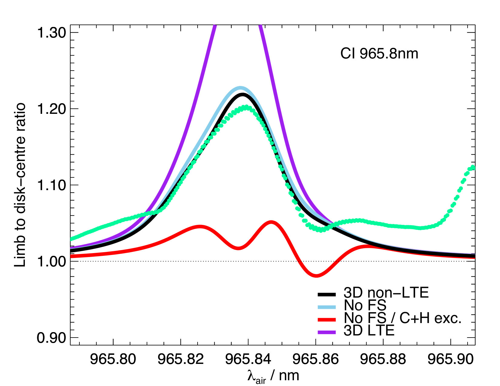 Figure 15
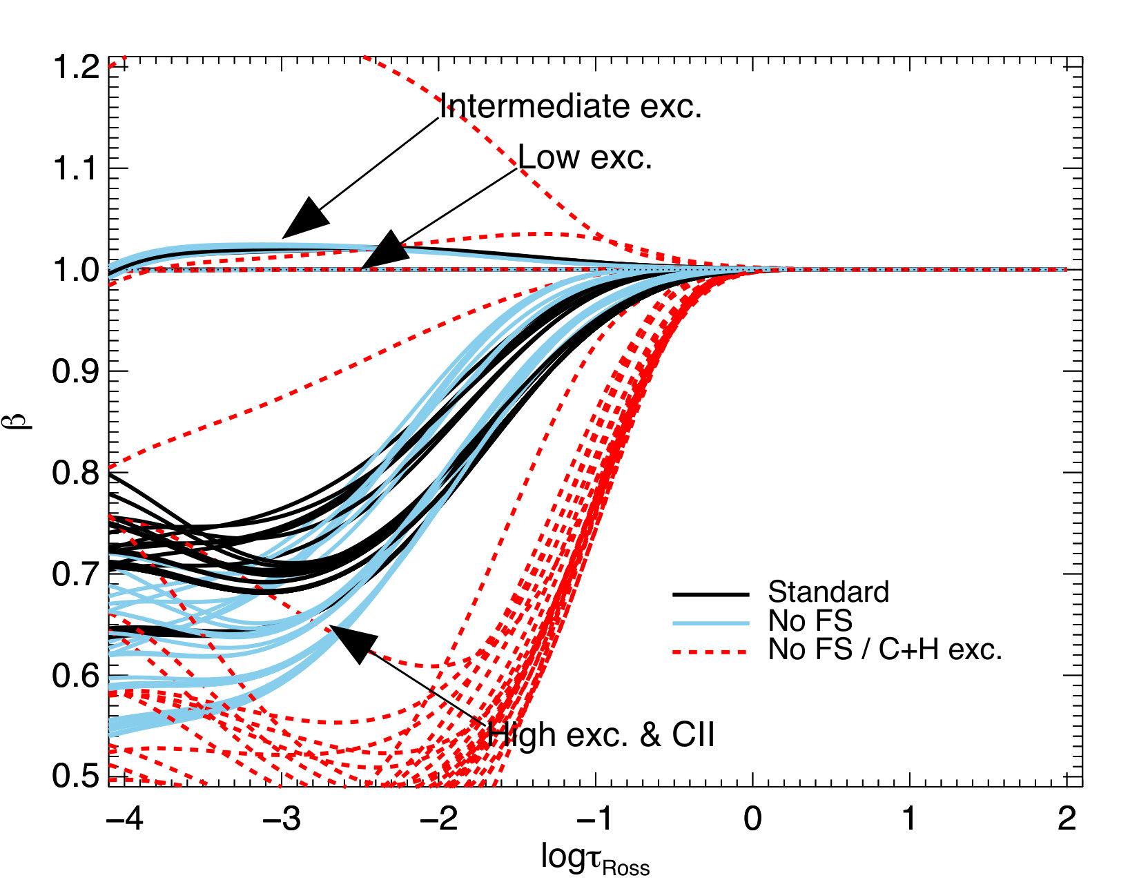 Figure 16
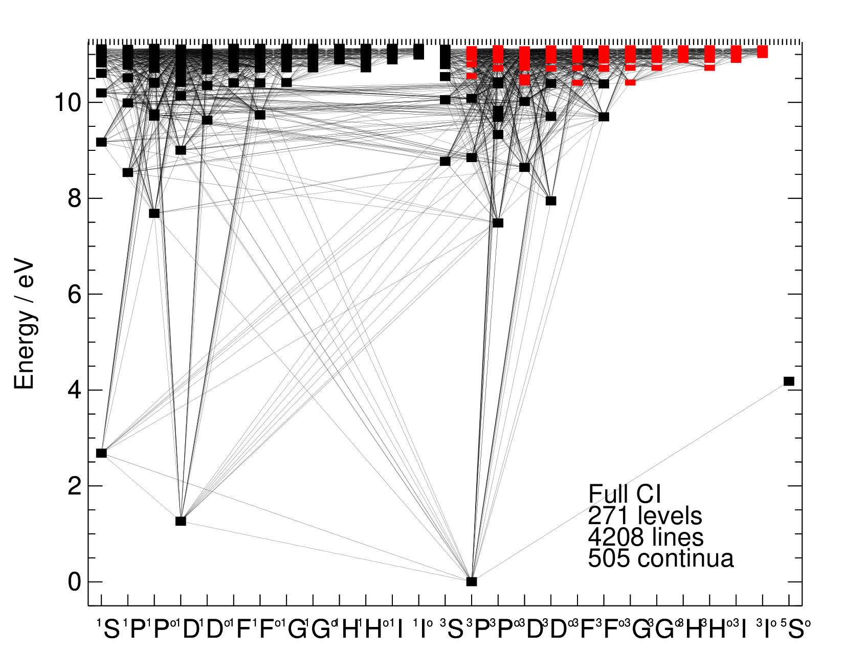 Figure 17
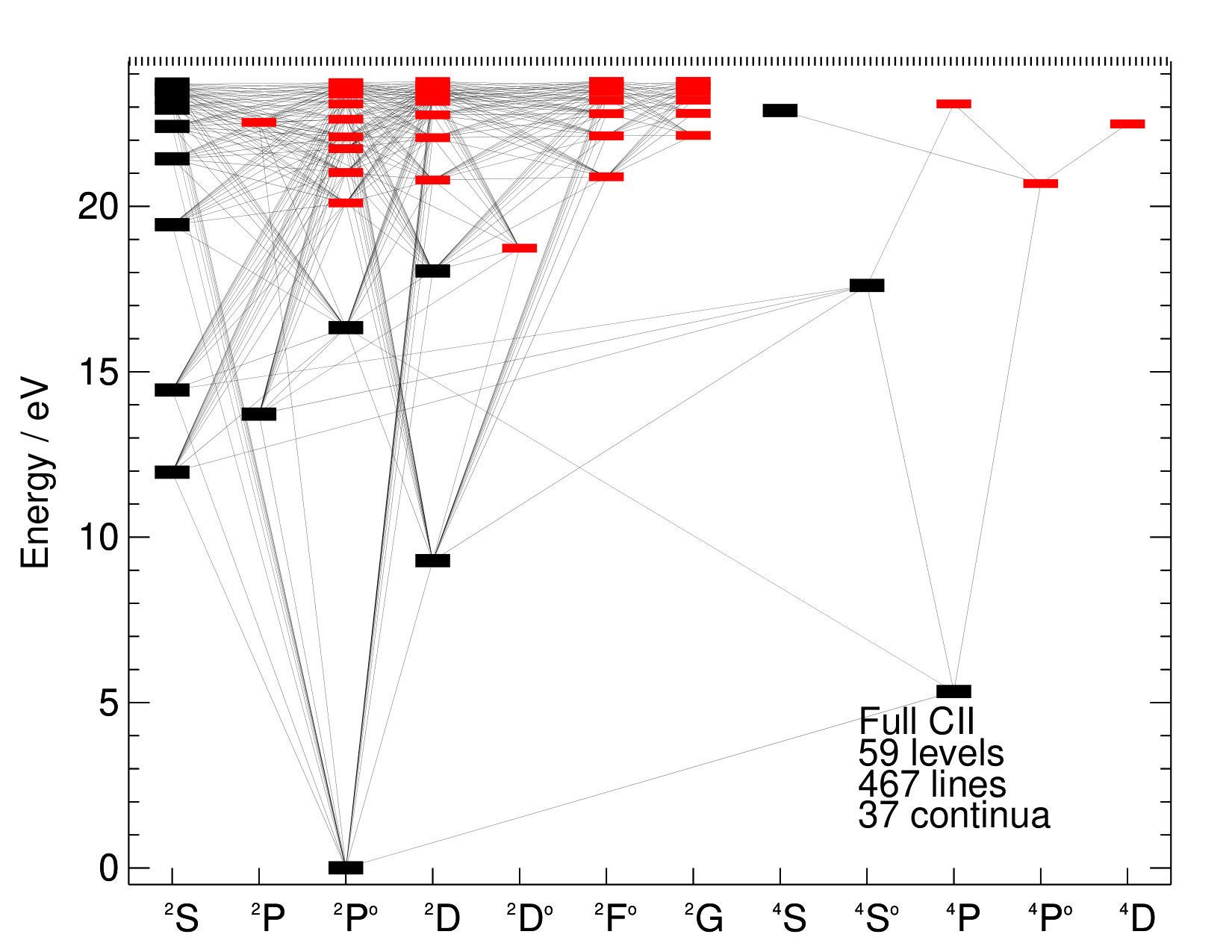 Figure 18
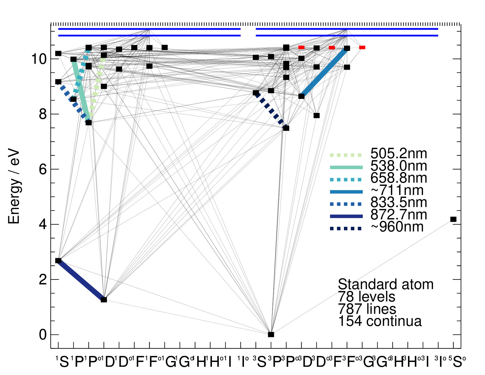 Figure 19
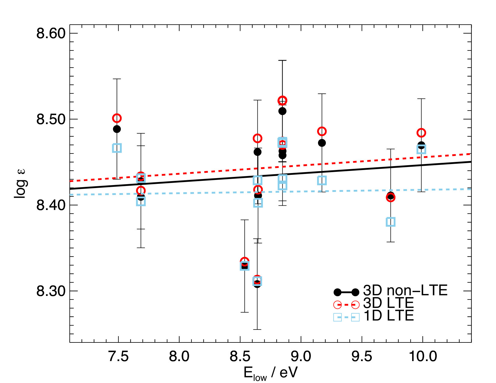 Figure 20
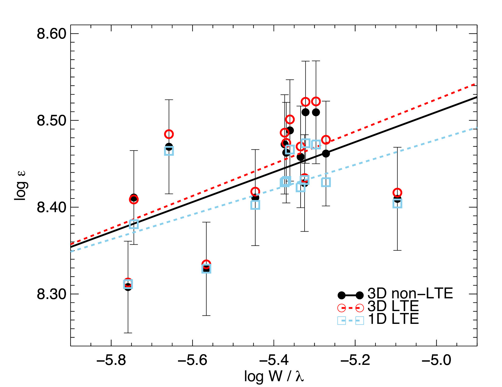 Figure 21
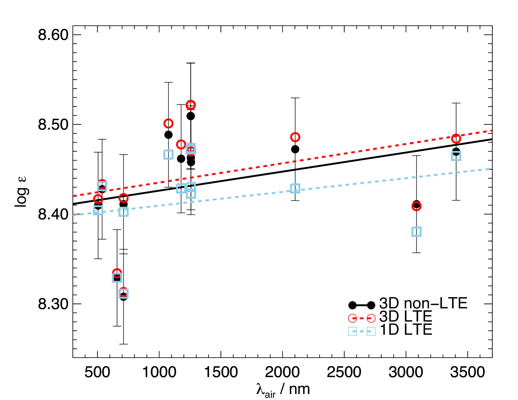 Figure 22
| Transition | |||||||||
|---|---|---|---|---|---|---|---|---|---|
| — | |||||||||
| — | |||||||||
| — | |||||||||
| — | |||||||||
| — | |||||||||
| — | |||||||||
| — | |||||||||
| — | |||||||||
| — | |||||||||
| — | |||||||||
| — | |||||||||
| — | |||||||||
| — | |||||||||
| — | |||||||||
| — | |||||||||
| — | |||||||||
| — | |||||||||
| — | |||||||||
| — | |||||||||
| — | |||||||||
| — | |||||||||
| — | |||||||||
| — | |||||||||
| — | |||||||||
| — | |||||||||
| — | |||||||||
| — | |||||||||
| — | |||||||||
| — | |||||||||
| — | |||||||||
| — | |||||||||
| — | |||||||||
| — | |||||||||
| — | |||||||||
| — | |||||||||
| — | |||||||||
| 3D non-LTE | No FS | No FS / C+H exc. | 3D LTE | 1D non-LTE | 1D LTE | |||
|---|---|---|---|---|---|---|---|---|
| Weighted mean | ||||||||
Peer Reviews
No public reviews on file for this paper yet. If you reviewed it on a platform where reviews are public (OpenReview, ICLR, NeurIPS, ICML), you can paste yours below so the community can read it here.
Videos
No videos yet. Explain this paper in a talk, walkthrough, or lecture? Add one.
11institutetext: Max Planck Institute für Astronomy, Königstuhl 17, D-69117 Heidelberg, Germany
11email: [email protected] 22institutetext: Theoretical Astrophysics, Department of Physics and Astronomy, Uppsala University, Box 516, SE-751 20 Uppsala, Sweden 33institutetext: Stellar Astrophysics Centre, Department of Physics and Astronomy, Aarhus University, Ny Munkegade 120, DK-8000 Aarhus C, Denmark 44institutetext: Centre Spatial de Liège, Université de Liége, avenue Pré Aily, 4031 Angleur-Liège, Belgium 55institutetext: Space Sciences, Technologies and Astrophysics Research (STAR) Institute, Université de Liège, Allée du 6 août, 17, B5C, 4000 Liège, Belgium 66institutetext: Research School of Astronomy and Astrophysics, Australian National University, Canberra, ACT 2611, Australia
3D non-LTE line formation of neutral carbon in the Sun
A. M. Amarsi 11
P. S. Barklem 22
R. Collet 33
N. Grevesse 4455
M. Asplund 66
Carbon abundances in late-type stars are important in a variety of astrophysical contexts. However C I lines, one of the main abundance diagnostics, are sensitive to departures from local thermodynamic equilibrium (LTE). We present a model atom for non-LTE analyses of C I lines, that uses a new, physically-motivated recipe for the rates of neutral hydrogen impact excitation. We analyse C I lines in the solar spectrum, employing a three-dimensional (3D) hydrodynamic model solar atmosphere and 3D non-LTE radiative transfer. We find negative non-LTE abundance corrections for C I lines in the solar photosphere, in accordance with previous studies, reaching up to around in the disk-integrated flux. We also present the first fully consistent 3D non-LTE solar carbon abundance determination: we infer , in good agreement with the current standard value. Our models reproduce the observed solar centre-to-limb variations of various C I lines, without any adjustments to the rates of neutral hydrogen impact excitation, suggesting that the proposed recipe may be a solution to the long-standing problem of how to reliably model inelastic collisions with neutral hydrogen in late-type stellar atmospheres.
Key Words.:
atomic data — radiative transfer — line: formation — Sun: abundances — Sun: photosphere
1 Introduction
As the second most abundant metal at the present epoch, carbon is interesting in a variety of astrophysical contexts. Via the C/O ratio, carbon has an oversized influence on the structure of the atmospheres (e.g. Madhusudhan, 2012) and interiors (e.g. Kuchner & Seager, 2005) of exoplanets. Carbon is similarly influential on the structure of the atmospheres (e.g. Gallagher et al., 2017) and interiors (e.g. Basu & Antia, 2008) of stars, and helps shape the properties of early stars (e.g Bromm & Loeb, 2003). Carbon is produced from a number of different sites including core collapse supernova (e.g. Woosley et al., 2002), AGB stars (e.g. Karakas, 2014), and Wolf-Rayet stars (e.g. Limongi & Chieffi, 2018); as such the Galactic Chemical Evolution of carbon is likely to be metallicity dependent and is still rather uncertain (e.g. Kobayashi et al., 2011).
Thus, accurate carbon abundances measured across the Galaxy are of great interest to the community. In late-type stars, C I lines are among the most commonly used carbon abundance diagnostics (e.g. Takeda et al., 2013; Nissen et al., 2014; Zhao et al., 2016), and can be measured down to 111. (e.g. Fabbian et al., 2009). However, in late-type stellar atmospheres, C I is sensitive to departures from local thermodynamic equilibrium (LTE; e.g. Vernazza et al., 1981; Stürenburg & Holweger, 1990; Takeda, 1992; Asplund et al., 2005; Takeda & Honda, 2005; Fabbian et al., 2006; Alexeeva & Mashonkina, 2015). For reliable results based on C I lines, non-LTE effects need to be taken into account.
A question to ask of non-LTE studies in general, is how realistic are the model atoms being used. For C I, the main uncertainties have hitherto been related to the completeness of the model atom (e.g. Stürenburg & Holweger, 1990), and to the treatment of neutral hydrogen impact excitation (e.g. Fabbian et al., 2006; Caffau et al., 2010; Alexeeva & Mashonkina, 2015). This latter point has lately been given considerable attention in the context of other elements. Lacking collisional cross-sections based on expensive quantum chemistry calculations of the molecular structure (e.g. Belyaev & Barklem, 2003; Belyaev et al., 2010, 2012), works have until recently typically either neglected neutral hydrogen impact excitation, or included them using the Drawin recipe (Drawin, 1968, 1969; Steenbock & Holweger, 1984; Lambert, 1993). This recipe however is not well-founded from a physical point of view, and is typically in error by orders of magnitude, with the errors going in different directions for different transitions (e.g. Barklem, 2016a, and references therein).
Recently, new recipes for neutral hydrogen impact excitation have become available that are both physically motivated and are relatively inexpensive to compute. In our study of neutral oxygen (Amarsi et al., 2018a), we suggested employing the asymptotic two electron model of Barklem (2016b), combined with the free electron model of Kaulakys (1991). These two models account for different physical mechanisms, with the asymptotic model particularly suitable for low level transitions while the free electron model should perform well for lines from intermediate- and high-excitation levels. Since the permitted optical and infrared C I lines are all in this regime, we expect that the mechanism represented by the free electron model is important here.
One way to validate model atoms is to use them in analyses of the solar spectrum. Trends in abundances inferred from spectral lines of different parameters (e.g. wavelength, line strength, excitation potential) have traditionally been used to probe errors in the modelling. More recently, centre-to-limb variations of spectral lines have been used to probe different recipes of neutral hydrogen impact excitation (Allende Prieto et al., 2004; Asplund, 2005; Pereira et al., 2009; Steffen et al., 2015; Lind et al., 2017; Amarsi et al., 2018a). This is because a) spectral lines observed at the limb form higher up than lines observed at disk-centre, b) free electrons are the main thermalising agents in the deep solar photosphere, and c) the relative importance of neutral hydrogen to free electrons as thermalising agents follows the ratio , which increases with height.
In order to use the Sun to validate atomic data in this way, one requires a reliable method for spectral line synthesis. The current state-of-the-art employs three-dimensional (3D) radiative-hydrodynamic model solar atmospheres, and 3D non-LTE post-processing radiative transfer (e.g. Amarsi et al., 2018a). To our knowledge, consistent 3D non-LTE calculations for C I in the solar photosphere that are based on a model atom that is sufficiently large for reliable abundance determinations have not been presented in the literature until now.
Here, we present a new model atom for C I line formation (Sect. 2), that uses a physically-motivated recipe for the rates of neutral hydrogen impact excitation. We carry out detailed 3D non-LTE calculations for C I lines in the solar photosphere, looking at disk-centre abundance trends as well as centre-to-limb variations of various clean C I lines in order to validate the model atom (Sect. 3). We discuss the implications on the solar carbon abundance and comment on the non-LTE effects on C I lines (Sect. 4). We close with a short summary (Sect. 5).
2 Method
2.1 Line-list
In Table 1 we list the 35 C I lines and single [C I] line for which 3D non-LTE line formation for the Sun were calculated and discussed in detailed (Sect. 3.2). This list was initially constructed by combining the set of lines given in Table 2 of Asplund et al. (2005), with the set of lines assigned a rank of in Table 1 of Caffau et al. (2010). The C I line was removed from this list on account of being very weak. The C I line was also removed, for having a very high excitation potential: the upper level of this transition was collapsed into a super level in the model atom, (Sect. 2.4.5), making the non-LTE effects predicted for this line less reliable. The C I , , , , and were added to this list because they are useful diagnostics in the metal-poor regime (Fabbian et al., 2009; Amarsi et al., 2019). We adopted different line parameters to those listed in Asplund et al. (2005) and Caffau et al. (2010) – in particular, using the oscillator strengths listed in the NIST Atomic Spectra Database (Sect. 2.4); the differences in the oscillator strengths are at most around .
For studying disk-centre abundance trends (Sect. 3.3), it is necessary to avoid lines that may be affected by solar and telluric blends in order to avoid biasing the results. Therefore, a subset of the lines in Table 1 was used. This subset is composed of of the C I lines as well as the single [C I] line presented in Table 2 of Asplund et al. (2005); we opted to remove the C I line because it is too strong to be a reliable abundance indicator, and the C I line because of difficulties in measuring its equivalent width. The adopted equivalent widths are those used in Asplund et al. (2009) (updated from Asplund et al. 2005), except for two lines: the C I and lines. These two lines are blended with faint CN lines; the new equivalent widths (Sect. 3.3) have taken these blends into account ( and respectively; J. Melendez priv. comm.).
For studying centre-to-limb variations (Sect. 3.4), another subset of the lines in Table 1 was used, due to the availability of high quality observational data. This subset is composed of the C I , , , , , , , and lines. Most of the infrared lines from Table 1 were not included because the analysis was based on the “SS3” atlas of Stenflo (2015) that only extends to . The other C I lines missing from this selection are, toward the limb, too contaminated by blends or are too difficult to continuum-normalise because of surrounding blends, to be useful here.
To aid intuition, in Fig. 1 we show the contribution functions of the intensity depression of the C I () and () lines, and the [C I] () line, at the two different values ( and ) considered in the centre-to-limb variation analysis (Sect. 3.4). These were computed in the same way as in Sect. 2.1.3 of Amarsi et al. (2018a); namely, by computing the full 3D contribution function (Amarsi, 2015, integrand of Eq. 12), after averaging over surfaces of equal optical depth and over time, and integrating over wavelength.
2.2 Radiative transfer code
The 3D non-LTE radiative transfer code balder (Amarsi et al., 2018b) was used. The code originated from multi3d (Botnen & Carlsson, 1999; Leenaarts & Carlsson, 2009), but has been developed and modified, utilising a new opacity package and other improvements for stellar abundance analyses. In this work, the underlying algorithm that solves the statistical equilibrum was replaced, from that presented in Sect. 2.3 of Rybicki & Hummer (1992), to that presented in Sect. 2.4 of that same paper. This was motivated by numerical issues in certain cases, namely of overlapping radiative transitions combined with relatively inefficient collisional coupling. The calculations on 1D model atmospheres were performed in the same way as the calculations on 3D model atmospheres, the only difference being the inclusion of microturbulent broadening in the 1D case (e.g. Gray, 2008, Chapter 17).
2.3 Model atmospheres
The 3D non-LTE radiative transfer calculations were performed in post-processing across eight snapshots, equally spaced in of solar time, of the same 3D radiative-hydrodynamic model solar atmosphere that was used in Amarsi et al. (2018a), calculated using the stagger code (Nordlund & Galsgaard, 1995; Stein & Nordlund, 1998; Collet et al., 2011). The mean effective temperature of the whole sequence , with a standard deviation of ; the mean effective temperature of the eight snapshots is also . For comparison the reference solar effective temperature is (Prša et al., 2016).
The calculations were performed for various carbon abundances in steps of , around a central value of (Asplund et al., 2009). Repeating the abundance analysis using steps of instead, resulted in inferred abundances that changed by at most (for the [C I] line).
For testing purposes, post-processing radiative transfer calculations were performed on the horizontally- and temporally-averaged 3D model solar atmosphere (hereafter ⟨3D⟩). The averaging was performed over the full sequence. This is the same ⟨3D⟩ model solar atmosphere that was used in Amarsi et al. (2018a). For interpreting the 3D effects, radiative transfer calculations were also performed on a 1D hydrostatic model solar atmosphere, which was calculated using the atmo code (Magic et al., 2013, Appendix A). The atmo model was constructed assuming a microturbulence of , and using the same equation of state and opacity binning scheme as used for the stagger model solar atmosphere, permitting a fair comparison.
For both the 1D and the ⟨3D⟩ model solar atmospheres, the post-processing radiative transfer calculations were performed for the same carbon abundances as were used on the 3D model solar atmosphere (i.e. in steps of , around a central value of ). These calculations were performed for a single, depth-independent microturbulence of .
2.4 Model atom
2.4.1 Overview
In this section we focus on the construction and reduction of the model atom for C I. The procedure is similar to that presented in Amarsi et al. (2018a) for O I. The model atom was constructed in two steps. In the first step, a comprehensive model atom was constructed, which we illustrate in Fig. 2. In the second step, the comprehensive model was reduced in complexity (Sect. 2.4.5), to generate what we refer to as the standard model atom, which we illustrate in Fig. 3. Reducing the size of the model atom is necessary to make the calculations presented here feasible; nevertheless the reduced model atom still encapsulates the relevant physics. In addition to the standard model atom, further models were used to test the sensitivity of the results to different ingredients and assumptions (Sect. 2.4.6).
In all cases, after the non-LTE iterations were completed on a reduced model atom, the final emergent intensities were calculated by applying the departure coefficients to the comprehensive model atom, taking care to preserve the total population number. In this way the final emergent intensities were based on accurate partition functions and the correct fine structure splitting, for higher accuracy.
2.4.2 Energy levels
We illustrate the structure of the comprehensive model atom in Fig. 2. Experimental fine structure energies were taken from the compilation of Moore (1993) via the NIST Atomic Spectra Database (Kramida et al., 2015), and, to make the model more complete, theoretical energies calculated under the assumption of pure LS coupling, from Luo & Pradhan (1989) for C I and Berrington & Seaton (1985) for C II via the Opacity Project online database (TOPbase; Cunto et al., 1993), were also used. Care was taken not to duplicate levels in the model, by using the NIST set only for lower lying levels (up to above the ground state for C I, and above the ground state for C II) and the TOPbase set for the remainder. The TOPbase energies were not extracted directly: instead, they were calculated from the stipulated effective principal quantum numbers, combined with the experimental ionisation limits from NIST. The C III ground state was also included in the comprehensive model atom.
2.4.3 Radiative transitions
Fine structure oscillator strengths were taken from Hibbert et al. (1993), Tachiev & Froese Fischer (2001), and Froese Fischer (2006) for C I, and Tachiev & Froese Fischer (2000) and Nussbaumer & Storey (1981) for C II, via NIST. For completeness this set was merged with theoretical oscillator strengths calculated under the assumption of pure LS coupling, from Luo & Pradhan (1989) for C I and Yan et al. (1987) for C II, via TOPbase. Photoionisation cross-sections were also taken from TOPbase, and smoothed over using a Gaussian filter (e.g. Bard & Carlsson, 2008). For all bound-bound transitions, natural broadening coefficients were calculated from the lifetimes stipulated in TOPbase. Where possible, collision broadening due to neutral hydrogen was calculated after the theory of Anstee, Barklem, and O’Mara (ABO), by interpolating the tables presented in Anstee & O’Mara (1995), Barklem & O’Mara (1997), and Barklem et al. (1998).
Where possible, the TOPbase radiative transitions that connect fine structure level(s) were split, using the relative strengths tabulated in Sect. 27 of Allen (1973). These tables are valid in the LS coupling regime, which is expected to be a good approximation for C I.
2.4.4 Collisional transitions
For electron impact excitation of C I, the rate coefficients presented by Wang et al. (2013) calculated under the B-spline R-matrix formalism (BSR e.g. Zatsarinny, 2006) were adopted where possible. The data set is complete up to ( above the ground state). The BSR data of Wang et al. (2013) were also used for electron impact ionisation of C I. Comparisons of BSR with independent methods for other species signal the reliability of this approach (e.g Barklem et al., 2017). Where the BSR data set is incomplete, the semi-empirical recipe of van Regemorter (1962) was used for excitation (imposing a minimum oscillator strength of ), while the empirical formula presented in Allen (1973) was used for ionisation.
For electron impact excitation of C II, included in the comprehensive model atom, the cross-sections presented by Wilson et al. (2005), calculated under the close-coupling R-matrix formalism (e.g. Burke & Robb, 1976), were adopted where possible. As for C I, this data set was completed using the semi-empirical recipe of van Regemorter (1962), while the empirical formula presented in Allen (1973) was used for electron impact ionisation of C II.
As we mentioned in Sect. 2.4.1, we adopt a new approach for neutral hydrogen impact excitation of C I. Following the approach of Amarsi et al. (2018a) for O I, the rate coefficients predicted by the asymptotic two-electron model, based on linear combinations of atomic orbitals (“LCAO”), of Barklem (2016b) were added to the rate coefficients predicted by the free electron model (“Free”), of Kaulakys (1991). We refer to this combined approach as “LCAO+Free”. The Barklem (2017) code was used to determine the rate coefficients in the latter case; these were redistributed among spin states following Eq. 8 and Eq. 9 of Barklem (2016a). The asymptotic two electron model was also used to calculate charge transfer between C I and neutral hydrogen (). Neutral hydrogen impact ionisation () was also included, through Eq. 8 of Kaulakys (1985), but was found to be of much lower importance.
Neutral hydrogen impact excitation of C II was neglected in the model. Neglecting these processes may in principle lead to overestimating the departures from LTE, and increase the influence of the statistical equilibrium of C II, on the C I line strengths. Ultimately however, we found that the overall influence of C II on C I lines is anyway small, (Sect. 2.4.5), so the exact treatment of these processes is unimportant here.
2.4.5 Standard model atom
The comprehensive model atom in Fig. 2 is too large to use in full 3D non-LTE radiative transfer calculations. It was therefore reduced, following a similar procedure to that described in Amarsi et al. (2018a) for our O I model atom. The reduction was performed in several steps as we outline below.
First, all of the excited C II levels as well as the C III level were removed. Tests revealed that these levels have only a very small impact on the C I line strengths: for the lines listed in Table 1, the differences in the equivalent widths in the emergent flux are negligible in the ⟨3D⟩ model solar atmosphere (much less than ). Previous studies have included several of the lower-lying C II levels (e.g. Fabbian et al. 2006 and Alexeeva & Mashonkina 2015 include the nine lowest C II levels, up to around above the C II ground state), which is more accurate but apparently not essential. The relative insensitivity of C II on the statistical equilibrium of C I can be understood from the high ionisation energy of C I (), which ensures that C I is the majority species in the solar photosphere; also, the first excited state of C II has a large separation from the ground state (), so that only the ground state of C II needs to be considered here.
Second, high-excitation C I levels ( above the ground state) that are closely separated in energy (within of each other) and that are within the same spin system, were collapsed into super levels. This is valid under the assumption that the composite levels are collisionally-coupled and therefore have identical departure coefficients. Within a super level, energies were weighted using their Boltzmann factors, adopting a temperature of that is characteristic of the line formation region. Transitions connected to super levels were collapsed into super transitions, in the way described in Amarsi & Asplund (2017). In the ⟨3D⟩ model solar atmosphere this reduction has an impact of around on the equivalent width in the flux in the worst case, the C I line of high excitation potential; for the other lines the impact is less than .
The resulting, reduced model atom is the standard atom used in this work. Abundance results and centre-to-limb variations are based on this model atom, unless otherwise indicated. We illustrate the model atom in Fig. 3.
2.4.6 Test atoms
For testing purposes, a further reduction was made to the standard model atom described in Sect. 2.4.5: namely, fine structure was collapsed following the method described in, for example, Amarsi & Asplund (2017). We refer to this as the “No FS” model. In the ⟨3D⟩ model solar atmosphere the equivalent widths in the fluxes of the lines were affected by up to . The error is lowest in the vertical intensity and grows for more inclined rays as the line formation moves outwards. For example, for the C I line that forms over a region extending high up in the atmosphere (Fig. 1), the error for is , while the error at is almost . In general, for abundance determinations from disk-integrated observations of late-type stars, errors of this magnitude are not significant; (for this reason, the “No FS” atom was used in our recent study of halo stars; Amarsi et al., 2019). However, for studying solar centre-to-limb variations, it is important to retain fine structure in the model atom.
To quantify the influence of neutral hydrogen impact excitation, a further model atom was constructed, wherein all neutral hydrogen impact excitation rate coefficients were set to zero. Given that fine structure has only a small impact on the statistical equilibrium, to reduce the computational cost fine structure was also collapsed in this test atom. We refer to this as the “No FS / C+H exc.” model.
3 Results
3.1 Departure coefficients
In Fig. 4 we illustrate departure coefficients across the ⟨3D⟩ model atmosphere, as predicted by the standard (reduced) model atom used throughout this study. There are broadly three groups of departure coefficients, corresponding to levels of low, intermediate, and high excitation potential; C II belonging to the last group. At solar metallicity, the departures from LTE are driven by photon losses in the many strong C I lines (e.g. Stürenburg & Holweger, 1990). There is a population cascade, that starts in the levels of high excitation potential and propagates down to the levels of intermediate excitation potential (, , and ), with levels of higher excitation potential underpopulating more. The low-excitation levels are all highly populated, and thus their populations are only marginally perturbed by this cascade (i.e. their departure coefficients stay close to unity).
We illustrate in Fig. 4 what happens when fine structure is collapsed in the model atom (“No FS”). As discussed in Sect. 2.4.5, fine structure has a small impact on the statistical equilibrium. It can be seen that in the regions , the departure coefficients are closer to unity in this case than in the standard case. This is because collapsing fine structure leads to stronger lines, that consequently form higher up in the solar atmosphere; therefore, the departures from LTE start to occur higher up in the solar atmosphere. However, it can also be seen that even higher up, , the departure coefficients are further from unity in this case than in the standard case. This is because, when fine structure is collapsed, the stronger lines have larger photon losses and thus drive larger departure from LTE.
We also illustrate in Fig. 4 what happens when neutral hydrogen impact excitation is neglected in the model atom (“No FS / C+H exc.”). Of all the collisional processes included in the model atom, these have the largest impact on the statistical equilibrium, generally acting to balance photon losses in the C I lines. When neutral hydrogen impact excitation is neglected, the departures from LTE set in much deeper in the atmosphere, with significant departures already at . It can also be seen that neutral hydrogen impact excitation is responsible for strong coupling within the different groups of levels (of low, intermediate, and high excitation potential).
3.2 3D/non-LTE abundance differences
To quantify the 3D non-LTE effects in the solar photosphere, equivalent widths were calculated for all of the lines listed in Table 1, using different modelling approaches (e.g. 3D non-LTE, 1D LTE). From these equivalent widths, abundance differences with respect to 3D non-LTE were calculated, by finding the abundance in, for example, the 1D LTE approach, that is needed to match the 1D LTE equivalent width to the 3D non-LTE equivalent width, for a fixed 3D non-LTE carbon abundance. We hereafter refer to these abundance differences as “abundance errors”, in contrast to the commonly used term “abundance corrections” that is understood to represent abundance differences with respect to 1D LTE. In Fig. 5 we illustrate these abundance errors that are based on equivalent widths, in the solar atmosphere, for the disk-centre intensity as well as for the disk-integrated flux.
In accordance with previous 1D non-LTE studies (Fabbian et al., 2006; Alexeeva & Mashonkina, 2015), the 3D LTE versus 3D non-LTE abundance errors, that quantify the non-LTE effects, are generally positive in both the disk-centre intensity and disk-integrated flux, reaching up to around in the latter. In other words, the non-LTE abundance corrections tend to be negative. There are trends in the middle and lower panels that indicate the departures from LTE are more severe for stronger C I lines (larger ), and for C I lines of intermediate excitation potential (–).
The reason why the abundance corrections are usually negative can be understood by looking again at the departure coefficients in Fig. 4. Levels of intermediate excitation potential do not depart severely from their LTE populations, whereas levels of high excitation potential are severely underpopulated with respect to LTE. Consequently, C I lines of intermediate excitation potential are subject to a source function effect (the ratio of the line source function to the Planck function follows ; Rutten, 2003). The line source function drops below the LTE expectation, and thus strengthens the C I lines with respect to LTE. Stronger lines are more susceptible to this effect, as their formation extends higher up into the atmosphere where the departures from LTE are greater.
Similarly, C I lines of high excitation potential are also susceptible to the source function effect. This is because higher levels show a larger underpopulation with respect to LTE (so still deviates from unity). For such lines, however, there is also a competing opacity effect ( drops below unity) that acts to weaken the C I lines with respect to LTE (the line strength follows the line opacity).
The [C I] line does not depart from LTE. This is expected because the lower and upper levels of the transition are both of low-excitation and are thus both highly populated (since C I is the majority species in the solar photosphere). They are therefore relatively insensitive to changes in the populations in the intermediate- and high-excitation C I levels.
We illustrate in Fig. 5 the sensitivity of the results to the treatment of fine structure, by presenting errors associated with collapsing all fine structure in the model atom (“No FS”). As anticipated (Sect. 2.4.6), the abundance errors are close to zero. They grow for stronger lines, which have significant line formation higher up in the photosphere where fine structure has a larger impact on the statistical equilibrium (as seen in Fig. 4).
We also illustrate in Fig. 5 the sensitivity of the results to neutral hydrogen impact excitation, by presenting errors associated with neglecting these processes (“No FS / C+H exc.”). These processes have only a small influence on the line strengths of the optical lines considered here: less than around on the fluxes in terms of abundances, at least in the Sun. Their influence is much larger on the near infrared lines (between and ) of intermediate excitation potential, where including them tends to weaken the lines considerably. For these lines the effects can reach up to around on the fluxes in terms of abundances, at least in the Sun. Neutral hydrogen impact excitation leads to closer coupling between the lower and upper levels of the near infrared lines (Sect. 3.1), and acts to reduce the source function effect described above.
Fig. 5 illustrates that the 1D non-LTE versus 3D non-LTE abundance errors, that quantify the 3D effects, are typically slightly smaller in magnitude than the non-LTE effects. However, these 3D effects go in the opposite direction to the non-LTE effects: they are mainly negative (corresponding to positive 3D abundance corrections, such that the 1D non-LTE C I lines are too strong, relative to 3D non-LTE). For the lines emergent at disk-centre, the differences are typically around , but can reach almost ; for the disk-integrated flux, the differences are less severe (less than ). Fig. 5 shows that, at disk-centre, the 3D effects are correlated with the line strengths () of the C I lines. Reducing the microturbulence only slightly alleviates the 3D effects on the lines. Rather, the 1D non-LTE versus 3D non-LTE abundance differences are caused by differences in the atmospheric stratification in 1D and in 3D; in support of this, we found that ⟨3D⟩ non-LTE versus 3D non-LTE abundance corrections are much less severe (less than at disk-centre).
Since the vast majority of spectroscopic stellar analyses today are based on 1D LTE, we also illustrate 1D LTE versus 3D non-LTE abundance errors in Fig. 5. As discussed above, the 3D effects and the non-LTE effects tend to go in opposite directions, at least for the C I lines considered in this work. Consequently, the 1D LTE versus 3D non-LTE abundance errors are intermediate between the negative 1D non-LTE ones (3D effects) and the positive 3D LTE ones (non-LTE effects). For the disk-centre intensity, they are always negative, which indicates that 3D effects are more important than non-LTE effects. On the other hand, for the disk-integrated flux, they tend to be positive, which indicates that non-LTE effects are more important than 3D effects. The middle row, second column of Fig. 5 reveals that the differences are typically of the order in the disk-integrated flux.
3.3 Abundance trends
In Table 2 we show our measured equivalent widths for the [C I] line and C I lines measured in the disk-centre intensity spectrum, together with the solar carbon abundances inferred from different modelling approaches. Uncertainties in the equivalent widths were assumed to be , after consideration of other published equivalent widths (Grevesse et al., 1991; Biemont et al., 1993; Asplund et al., 2005; Caffau et al., 2010). Uncertainties in the oscillator strengths (Table 1) were also folded into the error budget, simply assuming a one-to-one mapping of the error in to the error in , adopting the errors stipulated in NIST.
The mean abundances presented in the final row were then calculated after weighting individual lines in the usual way: . Under the assumption that all of the uncertainties are uncorrelated, the standard error in the weighted means presented in the final row is . The forbidden [C I] line was also included in this weighted mean (i.e. it was treated equally to the permitted C I lines). We discuss the mean abundance and its error further, in Sect. 4.2.
The 3D non-LTE versus 3D LTE abundance differences in Table 2 are not very severe: typically around . This can be contrasted with the values plotted in Fig. 5, which can be in excess of . This is because the lines selected for determining the solar carbon abundance are relatively insensitive to departures from LTE. Using the disk-centre intensity, rather than the disk-integrated flux, further reduces the impact of non-LTE effects. This means that the inferred solar carbon abundance should be less sensitive to any residual modelling errors arising from the non-LTE model atom and radiative transfer.
In Fig. 6 we illustrate the inferred solar carbon abundances as functions of different line parameters. These plots are a useful check of possible systematic errors in the models. However, they have less diagnostic power on different non-LTE models, owing to the large scatter in the inferred line-by-line abundances. For clarity, we only display the abundances inferred from the 3D non-LTE, 3D LTE, and 1D LTE models in these plots.
Using the 3D non-LTE model, consistent abundances are obtained from the different C I lines, within a standard deviation of . This large dispersion may indicate systematic errors in the models, rather than uncertainties in the equivalent width measurements. It is similar to the typical uncertainties in the individual oscillator strengths (Table 1), and could therefore be in part explained by errors in the oscillator strengths.
There is a slight trend in the inferred abundance with wavelength, and a more noticeable trend with line strength () that is significant at the level. Larger abundances tend to be inferred from the stronger C I lines than from the weaker ones. The trend is mainly driven by the very low abundances inferred from the two weak C I and lines, as observed previously by Asplund et al. (2005). To bring these two lines into agreement with the other lines, their values would need to be decreased by about , or around if the errors in Table 1 are to be believed. Improved C I oscillator strengths would be highly desirable to help resolve this issue.
3.4 Centre-to-limb variations
The centre-to-limb variations of a selection of C I lines (Sect. 2.1) were studied using the high-resolution, high signal-to-noise “SS3” atlas of Stenflo (2015) of the limb to disk-centre ratio atlas : {IEEEeqnarray}rCl r(μ)&≡ I(μ)/I^cont.(μ) ,
R(μ)≡r(μ)/r(1.0) .
Stenflo (2015) provide data continuously from roughly to , for , and state that the uncertainty in the viewing angle is at least .
The limb to disk-centre ratios predicted by a) the 3D non-LTE model, b) the 3D non-LTE model but collapsing all fine structure in the model atom (“No FS”), c) the 3D non-LTE model but neglecting collapsing all fine structure in the model atom and neglecting neutral hydrogen impact excitation (“No FS / C+H exc.”), and d) the 3D LTE model, were fit to the observations. The 1D models were not considered here for two reasons. First, we are mainly interested in comparing different non-LTE modelling approaches; this is best done using the 3D models. Second, the 1D models are complicated by the requirements of extra broadening, usually in the form of microturbulence and macroturbulence fudge parameters.
Prior to performing the fits, the atlas was renormalised using clean regions close to each C I line. When fitting each C I line, the absolute wavelength calibration of the atlas was treated as a free parameter. The viewing angle was permitted to vary freely within the assumed uncertainty of . For each line and each model, the solar carbon abundance was set to the values inferred from analysing the disk-centre equivalent widths, and was permitted to vary freely within an assumed uncertainty of . For most of the lines, the adopted disk-centre abundances can be found in Table 2. The C I , , and lines are missing from that table, as they are not ideal solar carbon abundance indicators (Sect. 2.1). Therefore, for these lines the abundance analysis presented in Sect. 3.3 was repeated, this time adopting disk-centre intensity equivalent widths from Asplund et al. (2005) for the C I line, and from Biemont et al. (1993) for the other two lines.
We illustrate the comparison of the model predictions to the observations for the different C I lines in Fig. 7 and Fig. 8. Not all of the lines studied have diagnostic power: the four different models predicted almost identical limb to disk-centre ratios for the C I and lines in the bottom row of Fig. 7, and for these two lines all four models are able to satisfactorily reproduce the observations.
As we mentioned in Sect. 2.1, the C I is blended with a CN line, that amount for around of the total disk-centre intensity equivalent width. The centre-to-limb variation of the molecular blend is different to that of the C I line, and this is reflected in the results for the C I in Fig. 8: the limb to disk-centre ratios of the different models are very similar, nevertheless, the ratio is slightly too strong compared to the observations (the discrepancy is more noticeable, when this plot is contrasted against the plot of the C I line in Fig. 7). We stress again that our equivalent width and inferred abundances in Table 2 have taken this blend into account.
The results for the C I , , and lines in Fig. 8 clearly favour the 3D non-LTE model over the 3D LTE model. This is evidence for the need to take departures from LTE into account, and for the accuracy of our model atom. The quality of the fits is not perfect, but this is understandable since the C I line is blended with a CN line in the far red wing, while the C I and C I lines clearly suffer from several small blends (including a Ti I line in the blue wing of the C I line), which is why they are not considered reliable abundance diagnostics.
The C I , , and lines in Fig. 8 show that the standard model atom, in which fine structure is retained, is able to fit the observations slightly better than the model atom in which fine structure is collapsed. This is as expected from the discussion in Sect. 2.4.6, with fine structure having a larger impact on the statistical equilibrium higher up in the atmosphere. Nevertheless, the difference between the two model predictions for the limb to disk-centre ratios is not very large.
Finally, it can be seen that neutral hydrogen impact excitation is indeed important in the solar photosphere. This is clearly demonstrated by the results for the C I , , and lines in Fig. 8, and also by the results for the C I and lines in Fig. 7. This result is interesting, given that the model adopts a new prescription for neutral hydrogen impact excitation (“LCAO+Free”), as described in Sect. 2.4.4.
4 Discussion
4.1 Comparison with previous studies
In Sect. 3.2, we found that the non-LTE abundance corrections for C I lines tend to be negative in the solar photosphere. This result can be compared with other 1D non-LTE analyses (e.g. Stürenburg & Holweger, 1990; Asplund et al., 2005; Fabbian et al., 2006; Caffau et al., 2010; Alexeeva & Mashonkina, 2015): these all predict negative non-LTE abundance corrections, in agreement with our result.
The most recent and comprehensive 1D non-LTE study is that of Alexeeva & Mashonkina (2015). They constructed a large model C I atom that included fine structure. In their later study (Alexeeva et al., 2016), they updated their model atom to include the more reliable BSR electron impact excitation and ionisation data (Zatsarinny, 2006), that was also adopted here, this had only a small impact on their results (Alexeeva, priv. comm.). The main difference between their model and that adopted here is the prescription for neutral hydrogen impact excitation: they adopted the Drawin recipe (Drawin, 1968, 1969; Steenbock & Holweger, 1984; Lambert, 1993), whereas the model used here adopted the “LCAO+Free” approach described in Sect. 2.4.4.
Comparing Fig. 2 of Alexeeva & Mashonkina (2015) with Fig. 4 here, the departure coefficients between the two studies are in good qualitative agreement. The low-excitation levels stay close to unity, the intermediate-excitation levels are slightly overpopulated with respect to LTE, and the high-exctation levels underpopulate with respect to LTE. As illustrated in Fig. 4 here, the extent of the departures from LTE are very sensitive to neutral hydrogen impact excitation, and this can explain for example the larger overpopulation of the intermediate-excitation levels compared to ours.
4.2 Solar carbon abundance
In Sect. 3.3 the solar carbon abundance was inferred from different C I lines as a diagnostic for the 3D non-LTE line formation models. We can also use this analysis to comment on the solar carbon abundance; a fully consistent 3D non-LTE determination has not been presented in the literature before.
Our derived abundance is . The value is the weighted mean from the fully consistent 3D non-LTE analysis presented in Table 2. The uncertainty was calculated in a way similar to the way explained in Sect. 4.1 of Scott et al. (2015): the systematic error arising from the non-LTE modelling was estimated by taking half the difference between the 3D LTE and 3D non-LTE results (), and the systematic error arising from the 3D modelling was estimated by taking half the difference between the 1D non-LTE and 3D non-LTE results (). These were combined in quadrature (). This systematic error was combined in quadrature with the standard error in the weighted mean (), to get the final uncertainty ().
Our derived value is consistent with the current standard value of (Asplund et al., 2009). In fact, it is in good agreement with the abundances inferred from each of the five different diagnostics employed in that work: the [C I] line (), C I lines (), CH lines (), CH lines (), and C2 lines ().
The [C I] line is insensitive to departures from LTE in the solar photosphere, and is relatively insensitive to the model atmosphere (see Asplund et al., 2009, Table 2). Most of the differences between the result of Asplund et al. (2009), of , and our result of , can be attributed to their larger oscillator strength: , compared to our , which leads to a difference in inferred abundance.
Our derived carbon abundance is significantly lower than the value of Caffau et al. (2010, 2011), who inferred . Their abundances were based on a 3D LTE analysis of the [C I] line and C I lines; as with Asplund et al. (2009), they applied negative 1D non-LTE versus 1D LTE abundance corrections for the C I lines.
The main reason for the discrepancy between our result and that of Caffau et al. (2010, 2011) can be traced to differences in the equivalent widths. Their equivalent widths tend to be systematically larger than those adopted here. Adopting their equivalent widths, and lines for that they assigned a rank of , we obtain a solar carbon abundance that is around larger than our derived value: that is, , in good agreement with their result. Looking carefully at the line shapes as well as databases of known lines in the solar spectrum, one can see that around two thirds of the C I lines used by Caffau et al. (2010, 2011) are blended, and are therefore not suitable abundance indicators, tending to bias the inferred carbon abundance upwards. Including blended lines also results in a significantly larger scatter in the results, with a standard deviation in the line-by-line carbon abundances of : compare Fig. 3 of Asplund et al. 2005 with Fig. 3 of Caffau et al. 2010, noting the difference in scales.
4.3 Solar C/O ratio
We briefly comment on the solar C/O ratio, having also recently presented a similar 3D non-LTE analysis of the O I triplet (Amarsi et al., 2018a). In that work, we obtained , in agreement with the current standard value (Asplund et al., 2009). Combining this with our value of , and assuming that these two uncertainties are uncorrelated, a solar C/O ratio of is inferred. This is consistent with the C/O ratios of Asplund et al. (2009), and also of Caffau et al. (2011), namely and respectively.
There remains a discrepancy with recent in-situ measurements of the fast solar wind from polar coronal holes: (von Steiger & Zurbuchen, 2016). We caution however that the C/O ratio in the solar wind may not be reflective of that in the solar photosphere owing to the First Ionisation Potential (FIP) effect and related fractionation effects (e.g. Serenelli et al., 2016). Nevertheless, current models suggest that such effects have only a small impact on the C/O ratio (e.g. Laming, 2015, Table 4), reflecting the similar ionisation potentials of neutral carbon and neutral oxygen.
On the other hand, this C/O ratio is larger than that measured in solar neighbourhood B-type stars. Nieva & Przybilla (2012) infer a larger oxygen abundance and a smaller carbon abundance from B-type stars, and infer a C/O ratio of , significantly lower than our solar estimate. The C/O ratio at the solar surface should roughly reflect that of the present-day local cosmos, and consequently that in short-lived B-type stars, because to first order carbon and oxygen are expected to be similarly affected by thermal diffusion, gravitational settling, and radiative acceleration, and should have had similar Galactic chemical enrichment histories (e.g. Asplund et al., 2009, and references therein). As discussed in Sect. 7.5 of Nieva & Przybilla (2012), a higher C/O ratio in the Sun compared to in nearby B-type stars is probably a sign that the Sun was born at a location closer to the centre of the Galaxy and later migrated outwards to its present location.
5 Conclusion
We have presented a new model atom for non-LTE analyses of C I line formation in late-type stars. We used the model atom together with detailed 3D non-LTE radiative transfer calculations across a 3D hydrodynamic model solar atmosphere, and analysed the solar spectrum. The model atom successfully reproduced the observed limb to disk-centre ratios of various C I lines, and conclusively ruled out 3D LTE as a viable model. We also presented the first consistent 3D non-LTE solar carbon abundance determination. Our derived value is . The new solar carbon abundance is consistent with the current standard value of presented in Asplund et al. (2009). Combined with an earlier 3D non-LTE solar oxygen abundance of , a solar C/O ratio of was inferred, again consistent with the current standard value of .
The true nature of inelastic collisions with neutral hydrogen, and their role on non-LTE stellar spectroscopy, is a decades-old problem. The main improvement in our model atom compared with previous studies is the more realistic, “LCAO+Free” description of neutral hydrogen impact excitation. This approach was first motivated in our earlier study of the solar centre-to-limb variation of the high excitation potential O I triplet (Amarsi et al., 2018a). As in that work, the 3D non-LTE line formation model in this work successfully reproduced the limb to disk-centre ratios of various C I lines, only when neutral hydrogen impact excitation was included. This suggests that the “LCAO+Free” recipe is a suitable approach for non-LTE modelling of neutral lines in late-type stars, although we cannot rule out some unknown, compensating systematic errors in our models. Since neglecting neutral hydrogen impact excitation can impart abundance errors of up to on disk-integrated fluxes, at least for C I lines in the Sun, it is important to take these collisional processes into account.
Acknowledgements.
We thank the referee, Lyudmila Mashonkina, for carefully reading and providing helpful suggestions on the manuscript, and in particular for insight and comments which helped identify a numerical issue with the code and thus greatly improved the paper. We also thank Sofya Alexeeva for answering in detail our various questions about her analysis, and Karin Lind and Amanda Karakas for comments on the manuscript. AMA acknowledges funds from the Alexander von Humboldt Foundation in the framework of the Sofja Kovalevskaja Award endowed by the Federal Ministry of Education and Research. PSB acknowledges support from the Swedish Research Council and the project grant “The New Milky Way” from the Knut and Alice Wallenberg Foundation. Funding for the Stellar Astrophysics Centre is provided by The Danish National Research Foundation (grant DNRF106). MA gratefully acknowledges funding from the Australian Research Council (grants DP150100250 and FL110100012). Some of the computations were performed on resources provided by the Swedish National Infrastructure for Computing (SNIC) at the Multidisciplinary Center for Advanced Computational Science (UPPMAX) and at the High Performance Computing Center North (HPC2N) under project SNIC2018-3-465. This work was supported by computational resources provided by the Australian Government through the National Computational Infrastructure (NCI) under the National Computational Merit Allocation Scheme.
The reference list from the paper itself. Each links out to its DOI / PubMed record.
- 1Alexeeva & Mashonkina (2015) Alexeeva, S. A. & Mashonkina, L. I. 2015, MNRAS, 453, 1619
- 2Alexeeva et al. (2016) Alexeeva, S. A., Ryabchikova, T. A., & Mashonkina, L. I. 2016, MNRAS, 462, 1123
- 3Allen (1973) Allen, C. W. 1973, Astrophysical quantities (London: University of London, Athlone Press, —c 1973, 3rd ed.)
- 4Allende Prieto et al. (2004) Allende Prieto, C., Asplund, M., & Fabiani Bendicho, P. 2004, A&A, 423, 1109
- 5Amarsi (2015) Amarsi, A. M. 2015, MNRAS, 452, 1612
- 6Amarsi & Asplund (2017) Amarsi, A. M. & Asplund, M. 2017, MNRAS, 464, 264
- 7Amarsi et al. (2018 a) Amarsi, A. M., Barklem, P. S., Asplund, M., Collet, R., & Zatsarinny, O. 2018 a, A&A, 616, A 89
- 8Amarsi et al. (2019) Amarsi, A. M., Nissen, P. E., Asplund, M., Lind, K., & Barklem, P. S. 2019, A&A, 622, L 4